Lipschitz Continuity of Signal Temporal Logic Robustness Measures:
Synthesizing Control Barrier Functions from One Expert Demonstration

Control barrier functions (CBFs) have emerged as a pre-eminent tool for controller synthesis for safety-critical systems [1, 2, 3, 4, 5, 6], due to their facilitation of robust, input-to-state-safe control [7, 8, 9], multi-agent control [10, 11], and learning-based control [12, 13], among other applications. In particular, CBFs are used to synthesize controllers that maintain forward invariance of a subset $\mathcal{C}$ of the system state space. Despite their tremendous success, synthesizing CBFs remains an open question with tremendous interest [14, 15, 16, 17, 18, 19]. Synthesis of CBFs is difficult, in large part because of two requirements these functions must satisfy: i) unit relative degree with respect to the controller, which is addressed in part via exponential barrier functions [20, 21], and ii) the differential inequality contingent on system dynamics that must hold over the entire state space [1].

These conditions can be expressed as constraints on optimization problems over function spaces, leading to learning-based approaches to identify these functions against provided models [14, 15, 16, 22]. However, these approaches tend to require a large amount of system data and suffer from a lack of generality to adapt to circumstances not reflected in the underlying data. To address these issues, recent work aims to construct these functions from first principles based on the expression of system behaviors in signal temporal logic (STL) [17, 18, 19, 23]. As such, they provide constructive approaches to transition between desired system behaviors and a quantifiable encoding of those behaviors through barrier functions. However, the synthesis of barrier functions developed in these prior works is not easily adaptable to changing scenarios — an issue we aim to resolve.

Before formally stating the problem, we provide a brief background on control barrier functions and signal temporal logic as they are central topics for the remainder of this paper.

The lemmas and theorems in this section will follow an inductive argument to prove that all specifications $\psi$ (6) have Lipschitz-continuous robustness measures. Our first lemma will prove the base case — that all STL atomic propositions $\mu$ as per (7) have Lipschitz robustness measures $h_{\mu}$.

Proof: First, for each proposition $\mu$, we define $\llbracket\mu\rrbracket$ as the set where $\mu$ holds and $\ell_{\mu}$ as the $2$-norm distance to that set.

Then, $h_{\mu}(x)=-\ell_{\mu}(x)$ satisfies both required conditions. $\mathbin{{\rule{5.38193pt}{5.38193pt}}}$

Proof: For $\psi_{3}=\neg\psi_{1}$, $\rho_{\psi_{3}}=\rho_{\psi_{1}}$ suffices, as $\rho_{\psi_{1}}$ is assumed to be Lipschitz with constant $L_{\psi_{1}}\geq 0$ and (semi)-norm $\|\cdot\|_{[a_{1},b_{1}]}$. The same holds for $\psi_{3}=\neg\psi_{2}$. For $\psi_{3}=\psi_{1}\wedge\psi_{2}$, $\rho_{\psi_{3}}(s)=\min\{\rho_{\psi_{1}}(s),\rho_{\psi_{2}}(s)\}$ is Lipschitz with constant $L_{\psi_{3}}=\max\{L_{\psi_{1}},L_{\psi_{2}}\}$ and (semi)-norm $\|\cdot\|_{\min\{a_{1},a_{2}\},\max\{b_{1},b_{2}\}}$. Likewise, for $\psi_{3}=\psi_{1}\lor\psi_{2}$, $\rho_{\psi_{3}}(s)=\max\{\rho_{\psi_{1}}(s),\rho_{\psi_{2}}(s)\}$ is Lipschitz with the same constant $L_{\psi_{3}}$ and (semi)-norm as prior. Proving these relations amounts to multiple applications of the Cauchy-Schwarz inequality while noting that $\min_{x\in X}f(x)=-\max_{x\in X}(-f(x))$ and that for arbitrary spaces $X$ and functions $f,g:X\to\mathbb{R}$, the following inequality is true:

$\mathbin{{\rule{5.38193pt}{5.38193pt}}}$

Proof: For notational ease, we abbreviate $|\rho_{\psi_{i}}(s,t)-\rho_{\psi_{i}}(z,t)|=\Delta_{i}(t)$ for signals $s,z\in\signalspace$. Consider the candidate robustness measure for $\psi_{3}$,

To prove that $\rho_{\psi_{3}}$ is Lipschitz, equation (12) is applied thrice, along with the fact $\min_{x\in X}~f(x)=-\max_{x\in X}(-f(x))$, to construct the following inequality:

Given that the component robustness measures $\rho_{\psi_{1}},\rho_{\psi_{2}}$ are Lipschitz, note that the inner arguments $\Delta_{2}(t^{\prime})$ and $\Delta_{1}(t^{\prime\prime})$ are dominated by their corresponding Lipschitz bounds. While the bound has only been assumed for signals $s,z$ evaluated at $t=0$, we note that the robustness evaluation of any signal $s^{\prime}\in\signalspace$ at some arbitrary time $\tilde{t}\in\mathbb{R}_{\geq 0}$ is such that $\rho(s^{\prime},\tilde{t})=\rho(s^{\prime\prime},0)$ where $s^{\prime\prime}(0)=s^{\prime}(\tilde{t})$. Setting $L_{\psi_{3}}=\max\{L_{\psi_{1}},L_{\psi_{2}}\}$, the following inequality is true:

thus completing the proof. $\mathbin{{\rule{5.38193pt}{5.38193pt}}}$

Proof: This proof follows an inductive argument. Consider the base case with specifications of the form $\psi=\mu_{1}\until_{[a,b]}\mu_{2}$ with $\mu_{1},\mu_{2}$ being propositions. Observe that $\psi$ has Lipschitz robustness measures with respect to (semi)-norms over $\signalspace$. This follows from Lemmas 1 and 3. Note that Lemma 1 proves that both propositions $\mu_{1},\mu_{2}$ have robustness measures that are Lipschitz continuous with respect to the $2$-norm $\|\cdot\|$. Furthermore, note that $\|\cdot\|_{[0,0]}=\|\cdot\|$. Therefore, applying Lemma 3 in the case where the two specifications have Lipschitz continuous robustness measures with respect to the signal (semi)norm $\|\cdot\|_{[0,0]}$ proves the base case. Lemmas 2 and 3 provide the inductive steps. As the base and inductive steps are true, this completes the proof. $\mathbin{{\rule{5.38193pt}{5.38193pt}}}$

We utilize these Lipschitz-continuous robustness measures for STL specifications to construct time-varying CBFs guaranteeing specification satisfaction to address Problem 1. At a high level, this approach requires an expert signal $s$ satisfying the desired system specification $\psi$, though how that signal is generated is left to the practitioner.

Proof: The first part of this proof will show that the candidate $h^{s}_{\psi}(x,t)$ as defined in equation (18) is a time-varying control barrier function. To show this, note that the Lie derivative $L_{g}h^{s}_{\psi}=\big(\frac{\partial h^{s}_{\psi}(x,t)}{\partial x}\big)^{\top}g(x)=\mathbf{0}^{\top}_{m}$ iff $\frac{\partial h^{s}_{\psi}(x,t)}{\partial x}=\mathbf{0}_{n}$. This is due to Assumption 1 and the rank-nullity theorem which implies that the nullspace of $g(x)$ is empty. As a result, we have two cases $\forall~(x,t)$, either (a) $L_{g}h^{s}_{\psi}(x,t)=\mathbf{0}_{m}$ or (b) $L_{g}h^{s}_{\psi}\neq\mathbf{0}_{m}$. In (a), the prior line of reasoning indicates that $x=s(t)$, which results in $\dot{h}^{s}_{\psi}(x,t)=0$ and $h^{s}_{\psi}(x,t)=\rho(s,0)\geq 0$. As a result, the differential inequality (2) collapses to $0\geq 0$ for any choice of class-$\mathcal{K}_{e}$ function $\alpha$. Therefore, any choice of input $u\in\mathbb{R}^{m}$ satisfies the differential inequality, so the supremum over all $u\in\mathbb{R}^{m}$ necessarily satisfies the same inequality. In case (b), $x\neq s_{t}$ and the following control input $u$ ensures that the inequality (2) holds for any class-$\mathcal{K}_{e}$ function $\alpha$:

where $(L_{g}h^{s}_{\psi})^{\dagger}$ is the pseudo-inverse of $L_{g}h^{s}_{\psi}$. Therefore, the supremum necessarily satisfies the same inequality. As the result holds in both cases for any choice of class-$\mathcal{K}_{e}$ function $\alpha$, $h^{s}_{\psi}(x,t)$ is a time-varying control barrier function.

The second part of this proof stems via Theorem 2. If for some signal $z$, $h^{s}_{\psi}(z(t),t)\geq 0,~\forall~t\in[0,T]$, then by (16),

By Definition 2 then, $z\models\psi$. $\mathbin{{\rule{5.38193pt}{5.38193pt}}}$

This section illustrates our method applied to generate a reactive path planner for a single-agent system [24]. Here, we represent the true system via a unicycle model, i.e. with system state $x\in\mathcal{X}\subseteq\mathbb{R}^{3}$ and control input $u\in\mathcal{U}\subset\mathbb{R}^{2}$:

Furthermore, we aim to generate a controller for this system that always identifies feasible paths to a goal, in a randomly generated maze-like setting with moving obstacles. More accurately, over a subset of the plane $\mathcal{W}=[-1.6,1.6]\times[-1,1]$, we define the set of considered operating environments $E$ as follows: (1) there must exist $8$ static obstacles occupying different cells in an $8\times 5$ evenly-spaced grid overlaid on $\mathcal{W}$; (2) the starting locations of $4$ moving obstacles $o_{i}\in\mathcal{W}$ and the ego agent’s initial state $x_{0}\in\mathcal{X}$ must occupy different cells and not exist within static obstacles; (3) there must exist $3$ goal cells for the agent with at least one feasible path existing to a goal at initialization — the center of each goal cell $g_{i}\in\mathcal{W}$; (4) the moving agents stop when they reach within $0.2$ meters of the ego agent, and can only progress in their motion if the agent moves away — this is to prevent faster-moving obstacles from crashing into the ego-agent without the agent having the ability to react. Figure 2 depicts an example setup of a valid environment $E$.

To formally define our specification $\psi$, we first define $SO\subset\mathcal{W}$ to be the set of planar centers of the $8$ static obstacles in our environment $E$. Second, we define $P_{\odot}:\mathcal{W}\to\mathbb{R}_{\geq 0}$ to be the path distance function defined as follows: (1) Identify the shortest feasible path — with respect to the number of cells that must be traversed — between the planar projection of the initial condition $x_{0}$ and a goal in the set $\odot\subset\mathcal{W}$; (2) record the center $c$ of the corresponding goal and output $\|w-c\|$. The formal system specification $\psi$ is as follows, with $\Pi=[\mathbf{I}_{2},\mathbf{0}_{2\times 1}]$:

The subformulas $B$ and $\psi_{\odot}$ are defined as follows:

• ($\psi_{\odot}$)

  Eventually make non-trivial progress towards the closest feasible goal in the set $\odot$ over a $10$ second period. Here $G=\{g_{1},g_{2},g_{3}\}$ corresponds to the randomly generated goals as part of the environment $E$ as previously described, and $H=\{h_{1},h_{2},h_{3},h_{4}\}$ corresponds to the centers of four home cells at the corners of the $8\times 5$ grid. Also, always avoid static and moving obstacles and treat moving obstacles to be frozen at the time instant of evaluation. Mathematically, a waypoint signal $\mathbf{w}$ taking values in $\mathcal{W}$ satisfies $\psi_{\odot}$ at time $t$, iff

  1. 1.

     $P_{\odot}(\Pi x_{0})-P_{\odot}(\mathbf{w}(t+10))\geq 0$, and

  2. 2.

     $\forall~t^{\prime}\in[t,t+10]$, $\min_{o\in SO}~\|\mathbf{w}(t^{\prime})-o\|_{\infty}\geq 0.2$m and $\min_{i=1,2,3,4}\|\mathbf{w}(t^{\prime})-o_{i}(t)\|\geq 0.18$m.

• ($B$)

  $B$ is an atomic proposition related to the existence of a basing signal. If the signal exists at time $t$ then $B(t)=\true$. If not, then $B(t)=\false$.

In short, $\psi$ represents the requirement that the system switch between two different sets of goals, $G$ and $H$, upon receiving a basing signal $B$, while also avoiding obstacles.

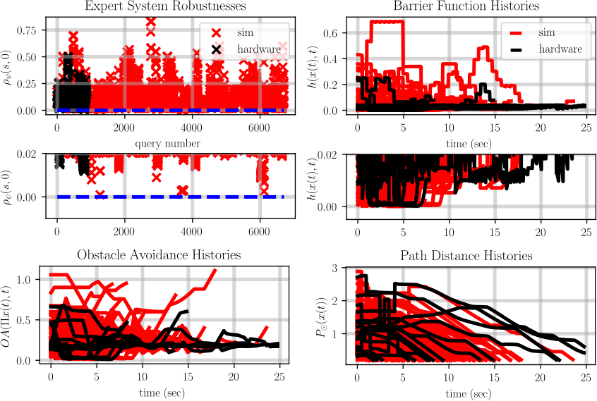
Notice that $\rho_{\psi}(s,0)\geq 0\iff(s,0)\models\psi$ insofar as we’re checking for positivity of the same conditions as expressed in the mathematical formalization of our specification $\psi$ (23). Furthermore, we also know that $\rho_{\psi}$ (28) is Lipschitz continuous when evaluated at time $t=0$ with constant $L_{\psi}=1$ and signal (semi)norm $\|\cdot\|^{Q}_{[0,10]}$. Here, $\|x\|^{Q}=\sqrt{x^{T}Qx}$ where $Q=\mathrm{diag}(\mathbf{I}_{2\times 2},0)$ and $\|s\|^{Q}_{[0,10]}=\max_{t\in[0,10]}\|s(t)\|^{Q}$. To show this, we know the obstacle avoidance function (25) is Lipschitz continuous with respect to the Euclidean $2$-norm over $\mathbb{R}^{2}$ and constant $L=1$. Here, we note that for any vector $v\in\mathbb{R}^{n}$, $\|v\|_{\infty}\leq\|v\|$. Second, the path difference function is also Lispchitz continuous with respect to the Euclidean $2$-norm over $\mathbb{R}^{2}$ and constant $L=1$. Then, the signal (semi)norm arises via the minimization over time in (28), noting that for any signal $z$ taking values in $\mathbb{R}^{n}$, $\|z(t+10)\|\leq\|z\|_{[0,10]}$ by Definition 3. Finally, we note that for any vector $v\in\mathbb{R}^{3}$, $\|v\|^{Q}\leq\|v\|$ and therefore for any signal $z$ taking values in $\mathbb{R}^{3}$, $\|z\|^{Q}_{[0,10]}\leq\|z\|_{[0,10]}$. As such, our robustness measure $\rho_{\psi}$ still satisfies the conditions of Theorem 2, though we note that using the signal (semi)norm $\|\cdot\|^{Q}_{[0,10]}$ as opposed to $\|\cdot\|_{[0,10]}$ increases performance as will be detailed below. As a result, our time-varying CBF according to Theorem 3 is as follows:

Through an inductive argument, we proved that every signal temporal logic specification has a Lipschitz continuous robustness measure with respect to a (semi)norm over the space of all signals. Leveraging this information, we provided a constructive method to determine control barrier functions for arbitrary systems and showcased the ability of these synthesized functions to realize the specification. For future work, we would first like to extend our existence results to outline a constructive method to determine these Lipschitz-continuous robustness measures. This would facilitate control barrier function synthesis. Second, as shown in the examples, repetitive signal generation and controller modification seem to generate reliable behavior. As such, there might be a potential interface with Model Predictive Control that we would like to explore. Finally, we would like to account for uncertainties to robustify hardware implementation.

References

- [1] A. D. Ames, X. Xu, J. W. Grizzle, and P. Tabuada, “Control barrier function based quadratic programs for safety critical systems,” IEEE Transactions on Automatic Control, vol. 62, no. 8, pp. 3861–3876, 2016.
- [2] S.-C. Hsu, X. Xu, and A. D. Ames, “Control barrier function based quadratic programs with application to bipedal robotic walking,” in 2015 American Control Conference (ACC). IEEE, 2015, pp. 4542–4548.
- [3] X. Xiong and A. Ames, “Slip walking over rough terrain via h-lip stepping and backstepping-barrier function inspired quadratic program,” IEEE Robotics and Automation Letters, vol. 6, no. 2, pp. 2122–2129, 2021.
- [4] M. Srinivasan, S. Coogan, and M. Egerstedt, “Control of multi-agent systems with finite time control barrier certificates and temporal logic,” in 2018 IEEE Conference on Decision and Control (CDC). IEEE, 2018, pp. 1991–1996.
- [5] J. Zeng, B. Zhang, and K. Sreenath, “Safety-critical model predictive control with discrete-time control barrier function,” in 2021 American Control Conference (ACC). IEEE, 2021, pp. 3882–3889.
- [6] J. Choi, F. Castaneda, C. J. Tomlin, and K. Sreenath, “Reinforcement learning for safety-critical control under model uncertainty, using control lyapunov functions and control barrier functions,” arXiv preprint arXiv:2004.07584, 2020.
- [7] S. Kolathaya and A. D. Ames, “Input-to-state safety with control barrier functions,” IEEE control systems letters, vol. 3, no. 1, pp. 108–113, 2018.
- [8] A. Alan, A. J. Taylor, C. R. He, G. Orosz, and A. D. Ames, “Safe controller synthesis with tunable input-to-state safe control barrier functions,” IEEE Control Systems Letters, vol. 6, pp. 908–913, 2021.
- [9] I. Tezuka and H. Nakamura, “Time-varying obstacle avoidance by using high-gain observer and input-to-state constraint safe control barrier function,” IFAC-PapersOnLine, vol. 53, no. 5, pp. 391–396, 2020.
- [10] Z. Cai, H. Cao, W. Lu, L. Zhang, and H. Xiong, “Safe multi-agent reinforcement learning through decentralized multiple control barrier functions,” arXiv preprint arXiv:2103.12553, 2021.
- [11] X. Tan and D. V. Dimarogonas, “Distributed implementation of control barrier functions for multi-agent systems,” IEEE Control Systems Letters, vol. 6, pp. 1879–1884, 2021.
- [12] Z. Marvi and B. Kiumarsi, “Safe reinforcement learning: A control barrier function optimization approach,” International Journal of Robust and Nonlinear Control, vol. 31, no. 6, pp. 1923–1940, 2021.
- [13] H. Ma, J. Chen, S. Eben, Z. Lin, Y. Guan, Y. Ren, and S. Zheng, “Model-based constrained reinforcement learning using generalized control barrier function,” in 2021 IEEE/RSJ International Conference on Intelligent Robots and Systems (IROS). IEEE, 2021, pp. 4552–4559.
- [14] P. Jagtap, G. J. Pappas, and M. Zamani, “Control barrier functions for unknown nonlinear systems using gaussian processes,” in 2020 59th IEEE Conference on Decision and Control (CDC). IEEE, 2020, pp. 3699–3704.
- [15] A. Robey, H. Hu, L. Lindemann, H. Zhang, D. V. Dimarogonas, S. Tu, and N. Matni, “Learning control barrier functions from expert demonstrations,” in 2020 59th IEEE Conference on Decision and Control (CDC). IEEE, 2020, pp. 3717–3724.
- [16] M. Srinivasan, A. Dabholkar, S. Coogan, and P. A. Vela, “Synthesis of control barrier functions using a supervised machine learning approach,” in 2020 IEEE/RSJ International Conference on Intelligent Robots and Systems (IROS). IEEE, 2020, pp. 7139–7145.
- [17] L. Lindemann and D. V. Dimarogonas, “Control barrier functions for signal temporal logic tasks,” IEEE control systems letters, vol. 3, no. 1, pp. 96–101, 2018.
- [18] ——, “Barrier function based collaborative control of multiple robots under signal temporal logic tasks,” IEEE Transactions on Control of Network Systems, vol. 7, no. 4, pp. 1916–1928, 2020.
- [19] X. Huang, L. Li, and J. Chen, “Multi-agent system motion planning under temporal logic specifications and control barrier function,” Control Theory and Technology, vol. 18, no. 3, pp. 269–278, 2020.
- [20] Q. Nguyen and K. Sreenath, “Exponential control barrier functions for enforcing high relative-degree safety-critical constraints,” in 2016 American Control Conference (ACC). IEEE, 2016, pp. 322–328.
- [21] V. Azimi and S. Hutchinson, “Exponential control lyapunov-barrier function using a filtering-based concurrent learning adaptive approach,” IEEE Transactions on Automatic Control, 2021.
- [22] C. Dawson, S. Gao, and C. Fan, “Safe control with learned certificates: A survey of neural lyapunov, barrier, and contraction methods,” arXiv preprint arXiv:2202.11762, 2022.
- [23] A. Donzé and O. Maler, “Robust satisfaction of temporal logic over real-valued signals,” in International Conference on Formal Modeling and Analysis of Timed Systems. Springer, 2010, pp. 92–106.
- [24] S. Wilson, P. Glotfelter, L. Wang, S. Mayya, G. Notomista, M. Mote, and M. Egerstedt, “The robotarium: Globally impactful opportunities, challenges, and lessons learned in remote-access, distributed control of multirobot systems,” IEEE Control Systems Magazine, vol. 40, no. 1, pp. 26–44, 2020.
- [25] P. Akella, A. Dixit, M. Ahmadi, J. W. Burdick, and A. D. Ames, “Sample-based bounds for coherent risk measures: Applications to policy synthesis and verification,” arXiv preprint arXiv:2204.09833, 2022.
- [26] P. Akella, M. Ahmadi, and A. D. Ames, “A scenario approach to risk-aware safety-critical system verification,” arXiv preprint arXiv:2203.02595, 2022.
- [27] A. Forsgren, P. E. Gill, and M. H. Wright, “Interior methods for nonlinear optimization,” SIAM review, vol. 44, no. 4, pp. 525–597, 2002.
- [28] C. Baier and J.-P. Katoen, Principles of model checking. MIT press, 2008.
- [29] G. E. Fainekos and G. J. Pappas, “Robustness of temporal logic specifications for continuous-time signals,” Theoretical Computer Science, vol. 410, no. 42, pp. 4262–4291, 2009.
- [30] O. Maler and D. Nickovic, “Monitoring temporal properties of continuous signals,” in Formal Techniques, Modelling and Analysis of Timed and Fault-Tolerant Systems. Springer, 2004, pp. 152–166.
- [31] T. G. Molnar, R. K. Cosner, A. W. Singletary, W. Ubellacker, and A. D. Ames, “Model-free safety-critical control for robotic systems,” IEEE robotics and automation letters, vol. 7, no. 2, pp. 944–951, 2021.
- [32] L. Lindemann and D. V. Dimarogonas, “Robust control for signal temporal logic specifications using discrete average space robustness,” Automatica, vol. 101, pp. 377–387, 2019.