The value of the information in the Moral Hazard setting

Ishak Hajjej Thanks: CREST $&$ IUT, LMBA, France, email ishak.hajjej@ensae.fr Caroline Hillairet Thanks: CREST, ENSAE Paris, France, email Caroline.Hillairet@ensae.fr Mohamed Mnif Thanks: ENIT, LAMSIN, University of Tunis El Manar, Tunis, Tunisia, email mohamed.mnif@enit.utm.tn

Abstract

This article studies the problem of evaluating the information that a Principal lacks when establishing an incentive contract with an Agent whose effort is not observable. The Principal ("she") pays a continuous rent to the Agent ("he"), while the latter gives a best response characterized by his effort, until a terminal date decided by the Principal when she stops the contract and gives compensation to the Agent. The output process of the project is a diffusion process driven by a Brownian motion whose drift is impacted by the Agent’s effort. The first part of the paper investigates the optimal stochastic control problem when the Principal and the Agent share the same information. This situation, known as the first-best case, is solved by tackling the Lagrangian problem. In the second part, the Principal observes the output process but she may not observe the drift and the Brownian motion separately. This situation is known as the second-best case. We derive the best response of the Agent, then we solve the mixed optimal stopping/stochastic control problem of the Principal under a fixed probability and on the filtration generated by the Brownian motion, which is larger than the one generated by the output process (that corresponds to the information available for the Principal). Under some regularity conditions, the Principal value function is characterized by solving the associated Hamilton Jacobi Bellman Variational Inequality. At the optimum, we prove that the two filtrations coincide. Finally, we compute the value of the information for the Principal provided by the observation of the Agent’s effort. It is defined as the difference between the principal value function in the first-best and second-best cases.

Keywords: Moral Hazard, Principal-Agent, stochastic control, optimal stopping, Hamilton Jacobi Bellman Variational Inequality, first-best case, second-best case .

MSC Classification : 60G40, 91B40, 91B70, 93E40.

Funding: This research is supported by a grant of the French National Research Agency (ANR), ”Investissements d’Avenir” (LabEx Ecodec/ANR-11-LABX-0047).

1 Introduction

A Principal-Agent problem concerns two individuals: a Principal (she) and an Agent (he). The Principal proposes a contract, which the Agent is free to accept or refuse, but neither part can change their mind. The Principal seeks to achieve two objectives. First, she wants the Agent to accept the contract. Second, the Principal wishes to extract the maximum profit from the contract. In game theory, such a situation forms what is called a Stackelberg game where the Principal is the leader and the Agent is the follower. There are many applications of the Principal-Agent problem, notably in finance (such as El Euch et al. [EMRT21] for market regulation), portfolio management (see Cvitanic et al. [CPT17]) and in the electricity markets (cf. Alasseur et al. [AEÉ+20] and more recently Aïd et al. [APT22]). Numerous situations in the economic literature lead to Principal Agent’s formulation, such as Public-Private Partnership (PPP) contracts. Auriol and Picard [AP13] discussed the appropriateness of PPP contracts when the public entity and the private operator do not share the same information about the cost parameter during the project life. Hajjej et al. [HHMP17] derived the optimal perpetual contract using techniques of stochastic control under partial information. Hajjej et al. [HHM22] proposed a similar modeling with a continuous payment in random horizon, by adding the possibility of stopping the contract at a random time, decided by the public.
In the literature, mainly three types of contracts are considered, according to the level of information.

•

The first type is commonly called the Risk-Sharing case or first-best case, in which the Principal and the Agent have access to exactly the same information. This case was studied, among others, by Borch [Bor92], Arrow [Arr64] and Wilson [Wil68]. In the exponential utility for both the Principal and the Agent, Muller [Mül97] showed that the optimal contract is a linear function of the output process terminal value. Cadenillas et al. [CCZ07] considered the case where the agent can control both the drift and the volatility of the output process. This work was followed by that of Cvitanic et al. [CWZ04] by using the maximum principle.
•

The second type is commonly called Moral Hazard or second-best case. This situation corresponds to the case where the Principal is unable to observe the action of the agent and she only observes the output process. The first paper on Principal Agent problems in continuous-time is the one of Holmstrom and Milgrom [HM87]. They considered a Brownian setting in which the agent controls the drift of the output process, and receives a lumpsum payment at the end of the contract, that is a finite time horizon. Schattler and Sung [SS93] generalized these results using dynamic programming and martingale methods. Cvitanic et al. [AP13], [Bel57] considered a general formulation in which the agent’s efforts impact both the drift and the volatility of the output process, using second-order BSDE in a non Markovian stochastic control setting.
•

The third type is commonly called Adverse Selection. This situation corresponds to the case where the principal does not fully know the characteristics of the agent. This type of problem has been studied by Sung [Sun05] then by Cvitanic and Zhang [CZ12] and Carlier et al. [CET07].

Compared to the first-best case, the second-best case corresponds to a Stackelberg game between the Principal and the Agent: the Principal proposes a contract, the Agent gives the best response characterized by his effort. Then, taking into account the optimal efforts, the Principal calculates the optimal contract that maximizes her utility. Some papers derived optimal Principal-Agent contracts in both situations of first-best and second-best, in the case where the Agent receives a terminal lumpsum payment and not a continuous rent. Mastrolia and Possamai [MP18] treated a Principal-Agent problem in the case where the Agent controls the drift of the output and with uncertainty on the volatility. In the first-best case, they showed that the optimal contracts are in a class of contracts linear with respect to the output and its quadratic variation. For the second-best case, they used Backward Stochastic differential equations (BSDE) to obtain a probabilistic representation of the agent value function. This representation characterizes the optimal action chosen by the agent. Aïd et al. [APT22] applied the Principal Agent problem in electricity markets. They showed that in the first-best case, the price of energy is a convex combination of the marginal value of energy for the consumer and the marginal cost for the producer. In the second-best case, the price of energy is non-constant and non-linear and is a decreasing function of time which induces more effort at the beginning of the period than at the end. In the setting of exponential utility for the Principal and the Agent, Muller [Mül97] showed that the optimal contract in the first-best case is linear in the final value of the output as in the second-best case.

The Principal faces a lack of information in the second-best case since she can not observe the effort of the Agent. Quantifying the value of an additional information has been investigated by some authors. Amendinger et al. [ABS03] considered a risk averse investor who maximizes his expected utility from terminal wealth with decisions based on the available information flow. This investor faces the opportunity to acquire some additional initial information. The value of this information is defined as the amount of money that he can pay for the additional information such that the investor is indifferent in the sense that his expected utility under optimal control is unchanged between paying nothing and not having the additional information and paying something and having the additional information. In other words, the value of the information is balanced out by the informational advantage in terms of maximal expected utility. In our case, the information is related to the knowledge of the effort of the Agent. The value of the information could be defined by the monetary amount that the Principal accepts to receive to compensate the lack of information. As the Principal is risk neutral, i.e. her utility function is linear, the monetary value of the information is then defined as the difference between the value function of the Principal in the first-best case and in the second-best case.

This paper considers a contract in which a risk neutral Principal proposes a continuous payment to a risk averse Agent until a random horizon decided by her to stop the contract. The Agent has the choice between accepting the contract and making an effort or refusing the contract if its reservation constraint is not satisfied. This work is related to the literature on dynamic contracting problems in continuous time. The first part of the paper is dedicated to the first-best case in which the Principal and the Agent have the same information: the two parts share the risk between themselves. The situation leads to a stochastic control problem with optimal stopping for a single individual "the Principal", who chooses both the rent and the efforts. The second part of the paper is dedicated to the second-best case. In particular, the Principal may not observe the effort of the Agent but only its impact on output process. In the literature, this problem is usually tackled using a weak approach : the output process follows a Brownian motion under a reference probability measure and the Agent changes the distribution of the output process by changing its drift; this induces a new probability measure, depending on the effort of the Agent, under which the problem is studied. For a given contract, the Agent optimizes his criterion on this probability measure, leading to the best response (effort) of the Agent. Then the Principal solves her problem under the law induced by the best response of the Agent, this is a standard mixed optimal stopping/stochastic control problem. Contrary to this weak formulation, we adopt in this paper a strong formulation. We fix a probability space, the Principal observes the output process, but she may not observe the drift nor the Brownian motion. The Principal and the Agent optimize their criteria under different information flow, the Agent’s filtration being larger than the Principal’s filtration. We are in the context of stochastic control under partial observation (see Bensoussan [Ben04]). We solve the mixed optimal stopping/stochastic control problem of the Principal on a larger set of controls that correspond to the adapted controls with respect to the total filtration which contains all information of the Principal and the Agent. At the optimum, we prove that the total filtration and the filtration generated by the output process coincide.

There are two contributions in this paper. First, we solve the Principal Agent Problem by using the strong approach in the non degenerate case i.e. the volatility of the output process is positive. Second, we compute the value of the information for the Principal provided by the observation of the Agent’s effort. The outline of the paper is as follows. In Section 2, we formulate the problem, using the strong approach and we define the Principal and the Agent problems, both in the first-best and second-best case. Section 3 is dedicated to the Principal-Agent problem in the first-best framework. In Section 4, we solve the Principal-Agent problem in the second-best case by determining the incentive compatible contract for the Agent and deriving the associated Hamilton Jacobi Bellman Variational Inequality associated to the Principal value function. Section 5 is dedicated to the numerical study.

2 Formulation of the Principal and Agent problem

Throughout the paper, let $\left(\Omega,\mathbb{F}=(\mathcal{F}_{t})_{t\geq 0},\mathbb{P}\right)$ be a filtered probability space where $\mathbb{F}=(\mathcal{F}_{t})_{t\geq 0}$ is the filtration (satisfying the usual conditions of right-continuity and completeness) generated by $W$ an one dimensional Brownian motion. We consider a time-continuous Principal-Agent problem where a risk-neutral Principal proposes a continuous payment to a risk-averse Agent until a random terminal horizon decided by the Principal. In return the Agent, if accepting the contract, makes an effort impacting the drift of the output process of the project. Throughout the paper, we adopt the strong formulation that is the Principal-Agent problem is solved under the reference probability measure $\mathbb{P}$ . A contract is a triplet $\Gamma=((R_{t})_{t},\tau,\xi)$ where $R$ is a non-negative rent, $\tau$ is the random terminal date of the contract (decided by the Principal) and $\xi$ is the cost of stopping the contract. The measurability of the triplet will be precised hereafter, depending on the situation considered (first-best or second-best case). Given a contract $\Gamma=((R_{s})_{s},\tau,\xi)$ offered by the Principal, the Agent gives a best response in terms of an effort $(A_{s})_{s\geq 0}$ which is an non-negative $\mathbb{F}$ -progressively measurable process. The Agent’s effort impacts the output process of the project, which is an $\mathbb{F}$ -progressively measurable process $(X_{s})_{s\geq 0}$ given by

X_{t}:=X_{0}+\int_{0}^{t}\varphi(A_{s})ds+\sigma W_{t},

(2.1)

where $X_{0}>0$ is the initial value of the output process. and $\sigma>0$ is the volatility (or diffusion coefficient), that is assumed to be constant. We introduce the following notations:

•

$\mathbb{F}^{X}:=(\mathcal{F}_{t}^{X})_{t\geq 0}$ is the filtration generated by the output process $X$ .
•

${\cal{T}}$ is the set of all $\mathbb{F}$ -stopping times.
•

${\cal{T}}^{X}$ is the set of all $\mathbb{F}^{X}$ -stopping times.

For the first-best case, the Principal and the Agent share the same information. A contract can be gathered into a quadruplet $((R_{t})_{t},\tau,\xi,A)$ , where the rent $R$ is is a non-negative ${\mathbb{F}}$ -progressively measurable process, $\tau\in{\cal{T}}$ , and $\xi$ is an non-negative ${\mathcal{F}}_{\tau}$ -measurable random variable. For the second-best case, the Principal observes the output process $X$ , but she does not observe directly the Agent’s effort. We are in the context of asymmetric information. Thus the information of the Principal is conveyed by the filtration $\mathbb{F}^{X}$ . A contract is then a triplet $\Gamma=((R_{t})_{t},\tau,\xi)$ where $R$ is a non-negative ${\mathbb{F}}^{X}$ -progressively measurable process, $\tau\in{{\cal T}^{X}}$ , and $\xi$ is a non negative ${\mathcal{F}}^{X}_{\tau}$ -measurable random variable¹¹ 1 This is in contrast with the weak formulation, in which the rent $R$ is an $\mathbb{F}$ -progressively measurable process, $\tau\in{\cal{T}}$ , and $\xi$ is ${\mathcal{F}}_{\tau}$ -measurable. Given a contract $\Gamma=((R_{s})_{s},\tau,\xi)$ offered by the Principal, the Agent gives a best response in terms of an effort process $A$ : this is a Stackelberg leadership model. The Agent accepts the contract only if his expected payoff at time $0$ exceeds his reservation value $\underline{x}>0.$
Let us now define the functions involved in the formulation of the optimization problems:

Assumption 2.1

$\bullet$

$\varphi$ is the function that models the marginal impact of the Agent’s efforts on the output process $\varphi:[0,\infty)\rightarrow[0,\infty)$ is $C^{2}$ strictly concave, bounded, increasing, $\varphi(0)=0$ and $\varphi^{\prime}(0)>0$ . We denote by $\|\varphi\|_{\infty}:=\sup_{a\geq 0}\varphi(a)$ .
$\bullet$

The utility function of the Agent $U:[0,\infty)\rightarrow[0,\infty)$ is $C^{2}$ strictly concave increasing and satisfying $U(0)=0$ and Inada’s conditions $U^{\prime}(\infty):=\displaystyle\lim_{x\longrightarrow\infty}U^{\prime}(x)=0,~U^{\prime}(0):=\displaystyle\lim_{x\longrightarrow 0}U^{\prime}(x)=\infty$ .
$\bullet$

$h$ is the cost of the effort for the Agent; $h:[0,\infty)\rightarrow[0,\infty)$ is $C^{2}$ , strictly convex increasing, $h(0)=0$ and $h^{{}^{\prime}}(0)>0$ .
$\bullet$

The time preference parameter of the Agent (resp. of the Principal) is a positive constant denoted $\lambda$ (resp. $\delta$ ). As the Principal is usually less impatient than the Agent, we assume that $\lambda\geq\delta$ .

Admissible Contracts:
We define the following sets of admissible contracts, depending on the information flow which will be used to solve the optimization problems of the Principal and the Agent in the first-best and second-best cases.
For the first-best case, and as the Principal and the Agent share the same information, the set of admissible strategies is defined as follows:

$\displaystyle\mathcal{E}$	$\displaystyle=$	$\displaystyle\{((R_{s})_{s\geq 0},\tau,\xi,(A_{s})_{s\geq 0})\mbox{ such that}~R_{s}\geq 0\mbox{ and }A_{s}\geq 0~ds\otimes d\mathbb{P}\mbox{ are }$	(2.2)
		$\displaystyle\mathbb{F}\mbox{-progressively measurable},~\tau\in\mathcal{T},\xi\geq 0~\mbox{is}~\mathcal{F}_{\tau}~\mbox{measurable},$
		$\displaystyle\mathbb{E}\left[\int_{0}^{\infty}e^{-\delta s}\|\varphi(A_{s})\|\vee e^{-\lambda s}\|h(A_{s})\|ds\right]<\infty,\mathbb{E}\left[\int_{0}^{\infty}e^{-\lambda s}\|U(\mathbb{R}_{s})\|\vee e^{-\delta s}\|R_{s}\|ds\right]<\infty,$
		$\displaystyle\mbox{ and }\mathbb{E}\left[e^{-\lambda\tau}U(\xi)\vee e^{-\delta\tau}\|\xi\|{{\mathbf{1}}_{\{\tau<\infty\}}}\right]<\infty\}.$

For the second-best case, we fix $\rho>0$ , and we introduce the following sets of admissible strategies for the Agent and for the Principal:

$\displaystyle\mathcal{D}^{Ag}_{\rho}$	$\displaystyle:=$	$\displaystyle\{(A_{s})_{s\geq 0}~\mathbb{F}~\mbox{-progressively measurable},~A_{s}\geq 0~ds\otimes d\mathbb{P}~a.e~\mbox{such that}~$	(2.3)
		$\displaystyle\mathbb{E}\left[\int_{0}^{\infty}e^{(\rho-2\lambda)s}\|h(A_{s})\|^{2}ds\right]<\infty~\mbox{and}~\mathbb{E}\left[\int_{0}^{\infty}e^{(\rho-2\delta)s}\|\varphi(A_{s})\|^{2}\right]<\infty\}$	(2.3)
$\displaystyle\mathcal{D}^{P}_{\rho}$	$\displaystyle:=$	$\displaystyle\{\big((R_{s})_{s\geq 0},\tau,\xi\big),\mbox{such that}~R\geq 0~\mbox{ is }\mathbb{F}^{X}\mbox{-progressively measurable},~\tau\in\mathcal{T}^{X}$	(2.4)
		$\displaystyle\xi\geq 0~\mbox{is}~\mathcal{F}_{\tau}^{X}~\mbox{measurable}~\mbox{such that }\mathbb{E}\left[\int_{0}^{\infty}e^{(\rho-2\lambda)s}\|U(R_{s})\|^{2}\vee e^{(\rho-2\delta)s}\|R_{s}\|^{2}ds\right]<\infty$
		$\displaystyle\mbox{and }\mathbb{E}\left[(e^{(\rho-2\lambda)\tau}U^{2}(\xi)\vee e^{(\rho-2\delta)\tau}\|\xi\|^{2}){{\mathbf{1}}_{\{\tau<\infty\}}}\right]<\infty\}.$

Objective function for the Agent and the Principal:
Given an admissible strategy $(\Gamma,(A_{s})_{s\geq 0})$ , where $\Gamma=((R_{s})_{s\geq 0},\tau,\xi)$ , the objective function of the risk-averse Agent is defined by the expectation under the probability $\mathbb{P}$ of his aggregate utility of the rent minus the cost of his effort plus the utility of the penalty when the contract is stopped, all these quantities being discounting using the Agent’s time preference parameter $\lambda$ :

J_{0}^{Ag}(\Gamma,A):=\mathbb{E}\left[\int_{0}^{\tau}e^{-{{{\lambda}}s}}(U(R_{s})-h(A_{s}))ds+e^{-{{\lambda}}\tau}U(\xi){{\mathbf{1}}_{\{\tau<\infty\}}}\right].

(2.5)

Using the Agent’s information flow $\mathbb{F}$ , his objective function starting from time $t$ is given by:

J_{t}^{Ag}(\Gamma,A):=\mathbb{E}\left[\int_{t}^{\tau}e^{-{{{\lambda}}(s-t)}}(U(R_{s})-h(A_{s}))ds+e^{-{{\lambda}}(\tau-t)}U(\xi){{\mathbf{1}}_{\{\tau<\infty\}}}\big|\mathcal{F}_{t}\right].

(2.6)

The objective function of the risk-neutral Principal is defined by the expectation under the probability $\mathbb{P}$ of the output process minus the rent paid to Agent minus the cost of stopping the contract, all these quantities being discounting using the Agent’s time preference parameter $\delta$ :

	$\displaystyle J_{0}^{P}(\Gamma,A)$	$\displaystyle:=$	$\displaystyle\mathbb{E}\left[\int_{0}^{\tau}e^{-\delta s}(dX_{s}-R_{s})ds-e^{-\delta\tau}\xi{{\mathbf{1}}_{\{\tau<\infty\}}}\right]$
		$\displaystyle=$	$\displaystyle\mathbb{E}\left[\int_{0}^{\tau}e^{-\delta s}(\varphi(A_{s})-R_{s})ds-e^{-\delta\tau}\xi{{\mathbf{1}}_{\{\tau<\infty\}}}\right].$

Using the Principal’s information flow $\mathbb{F}$ in the first-best case (resp. $\mathbb{F}^{X}$ in the second -best case), her objective function starting from time $t$ is given by:

	$\displaystyle J_{t}^{P,FB}(\Gamma,A)$	$\displaystyle=$	$\displaystyle\mathbb{E}\left[\int_{t}^{\tau}e^{-\delta(s-t)}(\varphi(A_{s})-R_{s})ds-e^{-\delta(\tau-t)}\xi{{\mathbf{1}}_{\{\tau<\infty\}}}\big\|\mathcal{F}_{t}\right].$
	$\displaystyle J_{t}^{P,SB}(\Gamma,A)$	$\displaystyle=$	$\displaystyle\mathbb{E}\left[\int_{t}^{\tau}e^{-\delta(s-t)}(\varphi(A_{s})-R_{s})ds-e^{-\delta(\tau-t)}\xi{{\mathbf{1}}_{\{\tau<\infty\}}}\big\|\mathcal{F}^{X}_{t}\right].$

Value function for the Principal in the first-best case:
Since the two parts share the same information, the Principal solves:

V_{0}^{FB}:=\displaystyle\sup_{(\Gamma,A)\in\mathcal{E}}J_{0}^{P}(\Gamma,A)

subject to the reservation constraint $J_{0}^{Ag}(\Gamma,A)\geq\underline{x}$ , where $\mathcal{E}$ is given by (2.2).

Value function for the Principal in the second-best case:
Given $\Gamma\in\mathcal{D}^{P}$ , the Agent solves

\sup_{A\in\mathcal{D}^{Ag}_{\rho}}J_{0}^{Ag}(\Gamma,A),

where $\mathcal{D}^{Ag}_{\rho}$ is given by (2.3). The public anticipates the Agent’s best response $A^{*}$ to propose the optimal contract and aims to solve:

V_{0}^{SB}:=\sup_{\Gamma\in\mathcal{D}^{P}}J_{0}^{P}(\Gamma,A^{*}),

subject to the reservation constraint $J_{0}^{Ag}(\Gamma,A^{*})\geq\underline{x}$ , where $\mathcal{D}^{P}$ is defined by (2.4).

Remark 2.2

The difference between the strong formulation and the weak formulation lies in the conditions of measurability. In the weak formulation, the objective function for the Agent and the Principal are computed under the probability measure induced by the effort of the agent (usually denoted by $\mathbb{P}^{A}$ ) and are both conditionally on $\mathcal{F}_{t}$ , while in the strong formulation, the objective functions are computed under $\mathbb{P}$ the objective function of Agent is, conditionally on $\mathcal{F}_{t}$ and the objective function of the Principal is, conditionally on $\mathcal{F}_{t}^{X}$ .

3 The first-best case

In this section, the Principal and the Agent share the same information. They observe both $X$ and the effort $A$ . We are in the context of risk sharing. They have to agree how to share the risk between themselves. We first rewrite the problem of the Principal in a more tractable stochastic control form. Then, we provide some properties related to the optimal contract. We distinguish two cases: either the Principal does not stop the contract i.e the infinite horizon case, or she could stop the contract.

3.1 The infinite horizon contract

The problem becomes a stochastic control problem for a single individual "the Principal", who chooses both the rent and the effort, under the reservation constraint. In this case, the Principal’s optimization problem is expressed as follows:

v(x)=\displaystyle\sup_{(R,\infty,0,A)\in\mathcal{E}}\mathbb{E}\left[\int_{0}^{\infty}e^{-\delta s}(\varphi(A_{s})-R_{s})ds\right]

(3.1)

subject to the reservation constraint

\mathbb{E}\left[\int_{0}^{\infty}e^{-{{{\lambda}}s}}(U(R_{s})-h(A_{s}))ds\right]\geq\underline{x}

(3.2)

We introduce a Lagrange multiplier $\lambda_{Lag}$ in order to solve this problem, and we consider the unconstrained problem:

	$\displaystyle\displaystyle\sup_{(R,\infty,0,A)\in\mathcal{E}}\left\{\mathbb{E}\left[\int_{0}^{\infty}e^{-\delta s}(\varphi(A_{s})-R_{s})ds\right]+\lambda_{Lag}(\mathbb{E}\left[\int_{0}^{\infty}e^{-\lambda s}(U(R_{s})-h(A_{s}))ds\right]-\underline{x})\right\}$
	$\displaystyle=\displaystyle\sup_{(R,\infty,0,A)\in\mathcal{E}}\mathbb{E}\left[\int_{0}^{\infty}e^{-\delta s}(\varphi(A_{s})-R_{s})ds+\lambda_{Lag}[e^{-\lambda s}(U(R_{s})-h(A_{s}))ds]\right]-\lambda_{Lag}\underline{x}.$

Proposition 3.1

Under Assumption 2.1, the solution of (3.1) under the reservation constraint (3.2) is given by²² 2 using the notation $x\vee y:=\max(x,y).$ :

R_{s}^{*}=(U^{\prime})^{-1}(\frac{1}{\lambda_{Lag}}e^{(\lambda-\delta)s})~\mbox{and}~A_{s}^{*}=(\frac{h^{\prime}}{\varphi^{\prime}})^{-1}(\frac{1}{\lambda_{Lag}}e^{(\lambda-\delta)s}){\vee 0}\,\mbox{ for all }s\in[0,\infty),

(3.3)

where the Lagrange multiplier $\lambda_{Lag}$ satisfies the following equation:

\int_{0}^{\infty}e^{-{{{\lambda}}s}}\left(U\left((U^{\prime})^{-1}(\frac{1}{\lambda_{Lag}}e^{(\lambda-\delta)s})\right)-h\left((\frac{h^{\prime}}{\varphi^{\prime}})^{-1}(\frac{1}{\lambda_{Lag}}e^{(\lambda-\delta)s}){\vee 0}\right)\right)ds=\underline{x}.

(3.4)

As a function of the time, the optimal rent $R^{*}$ is non-increasing and the optimal effort $A^{*}$ is non-decreasing.

This means that since the Agent is more impatient than the Principal, he will receive a higher rent and he will provide a smaller effort at the beginning of the contract than in the future.

Proof: We fix $s\in[0,\infty)$ . The function $x\longrightarrow-e^{-\delta s}x+\lambda_{Lag}e^{-\lambda s}U(x)$ is concave on $[0,\infty)$ . The first order condition for maximization on $(0,\infty)$ is given by:

\displaystyle-e^{-\delta s}+\lambda_{Lag}e^{-\lambda s}U^{{}^{\prime}}(x^{*})=0.

Here $\lambda_{Lag}$ must be positive, otherwise $e^{-\delta s}=0$ which is false. We deduce that the optimal rent is positive, deterministic and is given by:

\displaystyle R_{s}^{*}=(U^{\prime})^{-1}(\frac{1}{\lambda_{Lag}}e^{(\lambda-\delta)s}).

For the optimal effort, we consider on $(0,\infty)$ the function $x\longrightarrow-e^{-\delta s}\varphi(x)-\lambda_{Lag}e^{-\lambda s}h(x)$ , which is concave. The first order condition of optimality is given by

\displaystyle-e^{-\delta s}\varphi^{\prime}(x^{*})-\lambda_{Lag}e^{-\lambda s}h^{{}^{\prime}}(x^{*})=0,\mbox{ if }x^{*}>0

otherwise $x^{*}=0$ . We deduce that the optimal effort is non-negative, deterministic and is given by:

\displaystyle A_{s}^{*}=(\frac{h^{\prime}}{\varphi^{\prime}})^{-1}(\frac{1}{\lambda_{Lag}}e^{(\lambda-\delta)s})\vee 0.

The linear independence constraint qualification is satisfied as $U^{\prime}({R^{*}_{s}})$ and $h^{\prime}({A^{*}_{s}})$ are positive. From Assumption 2.1, and since $\varphi$ and $U$ are strictly concave, $h$ is strictly convex, then we have

\displaystyle\left\{\begin{array}[]{ll}e^{-\delta t}\varphi^{{}^{\prime\prime}}({A^{*}_{s}})-\lambda_{Lag}e^{-\lambda t}h^{{}^{\prime\prime}}({A^{*}_{s}})<0,\\ \lambda_{Lag}e^{-\lambda t}U^{{}^{\prime\prime}}({R^{*}_{s}})<0,\end{array}\right.

and so the sufficient conditions of optimality are satisfied. The optimal rent and the optimal effort are deterministic controls given by (3.3).
It follows that:

			$\displaystyle\mathbb{E}\left[\int_{0}^{\infty}e^{-{{{\lambda}}s}}(U(R_{s}^{})-h(A_{s}^{}))ds\right]$		(3.6)
		$\displaystyle=$	$\displaystyle\int_{0}^{\infty}e^{-{{{\lambda}}s}}\left(U\left((U^{\prime})^{-1}(\frac{1}{\lambda_{Lag}}e^{(\lambda-\delta)s})\right)-h\left((\frac{h^{\prime}}{\varphi^{\prime}})^{-1}(\frac{1}{\lambda_{Lag}}e^{(\lambda-\delta)s})\vee 0\right)\right)ds.$		(3.6)

The first order condition with respect to $\lambda_{Lag}$ is given by the complementary condition i.e.

\lambda_{Lag}\Big(\mathbb{E}\left[\int_{0}^{\infty}e^{-\lambda s}(U(R_{s}^{*})-h(A_{s}^{*}))ds\right]-\underline{x}\Big)=0.

Since $\lambda_{Lag}>0$ and using (3.6), we obtain Equation (3.4) satisfied by $\lambda_{lag}$ (the reservation constraint is binded). The monotonicity of $s\rightarrow R_{s}^{*}=(U^{\prime})^{-1}(\frac{1}{\lambda_{Lag}}e^{(\lambda-\delta)s})$ (non-increasing) and of $s\rightarrow A_{s}^{*}=(\frac{h^{\prime}}{\varphi^{\prime}})^{-1}(\frac{1}{\lambda_{Lag}}e^{(\lambda-\delta)s})\vee 0$ (non-decreasing) is a direct consequence of the increase of $s\rightarrow e^{(\lambda-\delta)s}$ (since $\lambda\geq\delta$ ), the decrease of $(U^{\prime})^{-1}$ (since $U$ is concave) and the increase of $(\frac{h^{\prime}}{\varphi^{\prime}})^{-1}$ (since $h$ is convex and $\varphi$ is concave). If $\lambda>\delta$ then $s\rightarrow R_{s}^{*}$ is decreasing. $\bullet$

Example 3.2

Suppose that the functions $\varphi$ and $h$ are given by $\varphi(x)=3(1-\exp(-\alpha x))$ and $h(x)=\exp(\beta x)-1.$ Then $\varphi^{\prime}(x)=3\alpha\exp(-\alpha x),~h^{\prime}(x)=\beta\exp(\beta x)$ , which implies that $\frac{h^{\prime}}{\varphi^{\prime}}(x)=\frac{\beta}{3\alpha}\exp((\beta+\alpha)x)$ , and so $(\frac{h^{\prime}}{\varphi^{\prime}})^{-1}(x)=\frac{1}{\alpha+\beta}\log(\dfrac{3\alpha}{\beta}x)$ . In the case of power utility function, i.e. $U(x)=cx^{p}$ (0<p<1) and so $(U^{\prime})^{-1}(x)=(\frac{x}{pc})^{\frac{1}{p-1}}$ , (3.3) yields the expressions

{R_{t}^{*}=\frac{1}{(pc\lambda_{Lag})^{\frac{1}{p-1}}}\exp\left(\frac{(\lambda-\delta)t}{p-1}\right)}\,\mbox{ and }A^{*}_{t}=\frac{1}{\alpha+\beta}\log\left(\frac{3\alpha}{\beta\lambda_{Lag}}\exp((\lambda-\delta)t)\right){\vee 0}.

If $\lambda_{Lag}\leq 3\frac{\alpha}{\beta}$ , then $A^{*}_{t}=\frac{1}{\alpha+\beta}\log\left(\frac{3\alpha}{\beta\lambda_{Lag}}\exp((\lambda-\delta)t)\right)$ for all $t$ .

\hskip-28.45274pt\mbox{ If }\lambda_{Lag}>3\frac{\alpha}{\beta},\mbox{ then }A^{*}_{t}=\left\{\begin{array}[]{ll}0&\mbox{ for }(\lambda-\delta)t\leq-\log\left(\frac{3\alpha}{\beta\lambda_{Lag}}\right)\\ \frac{1}{\alpha+\beta}\log\left(\frac{3\alpha}{\beta\lambda_{Lag}}\exp((\lambda-\delta)t)\right)&\mbox{ for }(\lambda-\delta)t>-\log\left(\frac{3\alpha}{\beta\lambda_{Lag}}\right).\end{array}\right.

The Lagrange multiplier $\lambda_{Lag}$ is solution to equation (3.6) (which has two different expressions depending on the interval considered)

\left\{\begin{array}[]{ll}\dfrac{c}{(pc\lambda_{Lag})^{\frac{p}{p-1}}(\lambda-\frac{p}{p-1}(\lambda-\delta))}+\frac{1}{\lambda}-\left(\frac{3\alpha}{\beta\lambda_{Lag}}\right)^{\frac{\beta}{\alpha+\beta}}\dfrac{\alpha+\beta}{\lambda\alpha+\beta\delta}&=\underline{x}\mbox{ on }[0,3\frac{\alpha}{\beta}]\\ \dfrac{c}{(pc\lambda_{Lag})^{\frac{p}{p-1}}(\lambda-\frac{p}{p-1}(\lambda-\delta))}+\left(\frac{1}{\lambda}\left(\frac{3\alpha}{\beta\lambda_{Lag}}\right)^{\frac{\lambda}{\lambda-\delta}}-\dfrac{\alpha+\beta}{\lambda\alpha+\beta\delta}\left(\frac{3\alpha}{\beta\lambda_{Lag}}\right)^{\frac{\lambda}{\lambda-\delta}}\right)\mathbf{1}_{\lambda\neq\delta}&=\underline{x}\mbox{ on }]3\frac{\alpha}{\beta},+\infty[.\end{array}\right.

3.2 The general case

In the first-best framework, and in the general case, the Principal is faced with the following optimization problem:

\displaystyle\displaystyle\sup_{(R,\tau,\xi,A)\in\mathcal{E}}\mathbb{E}\left[\int_{0}^{\tau}e^{-\delta s}(\varphi(A_{s})-R_{s})ds-e^{-\delta\tau}\xi\right],

(3.7)

where $\mathcal{E}$ is given by (2.2), and subject to the reservation constraint

\mathbb{E}\left[\int_{0}^{\tau}e^{-\lambda s}(U(R_{s})-h(A_{s}))ds+e^{-\lambda\tau}U(\xi)\right]\geq\underline{x}.

The main result of Section 3 is the following proposition. It gives the possible cases in the first-best case.

Proposition 3.3

Under Assumption 2.1, in the first-best case, we define the function

t\longrightarrow H_{t}:=\varphi(A_{t}^{*})-R_{t}^{*},

where $A^{*}$ and $R^{*}$ are given in (3.3). Then

1.

If $\int_{0}^{\infty}e^{-\delta s}H_{s}ds>0$ , it is not optimal for the Principal to end the contract ( $\tau^{*}=\infty$ is optimal).
2.

If $\int_{0}^{\infty}e^{-\delta s}H_{s}ds\leq 0$ , the Principal does not offer the contract to the Agent ( $\tau^{*}=0$ is optimal).

Proof: We introduce the Lagrangian problem. The first order conditions inside the expectation with respect to the effort and the rent are the same as in the infinite horizon contract. We know that $\lambda_{Lag}\geq 0$ . If $\lambda_{Lag}=0$ , then as in the proof of the infinite horizon case, we deduce that for all $t\geq 0$ , we have $R^{*}_{t}=0$ , $A^{*}_{t}=0$ (and $H(t)=0$ for all $t$ ). It is then clear that we must have $\tau=0$ otherwise the reservation constraint is never satisfied .
For $\lambda_{Lag}>0$ , the function $t\longrightarrow H_{t}$ is well-defined.
Since $\lambda\geq\delta$ , $t\mapsto\frac{1}{\lambda_{Lag}}e^{(\lambda-\delta)t}$ is non-decreasing. The strict concavity of the function $\varphi$ and the strict convexity of the function $h$ yields the function $t\rightarrow(\frac{h^{\prime}}{\varphi^{\prime}})^{-1}(\frac{1}{\lambda_{Lag}}e^{(\lambda-\delta)t})$ is non-decreasing. The strict concavity of $U$ and the decrease of $U^{\prime}$ yields that the function $t\rightarrow(U^{\prime})^{-1}(\frac{1}{\lambda_{Lag}}e^{(\lambda-\delta)t})$ is non-increasing. Therefore the optimal rent is non-increasing and the optimal effort is non-decreasing in time. By monotonicity of the function $\varphi$ , the function $t\rightarrow H_{t}$ is non-decreasing.
We have the following cases:
First case: If $H_{0}>0$ , and since $U^{-1}$ in non-negative, as in Proposition 3.1, it is optimal for the Principal to never stop the contract ( $\tau=\infty$ is optimal).
Second case: If $H_{0}\leq 0$ , and if there exists a $t_{0}$ such that $H_{t_{0}}=0,$ we compute: $\int_{0}^{t_{0}}e^{-\delta s}H_{s}ds$ and $\int_{t_{0}}^{\infty}e^{-\delta s}H_{s}ds.$

1.

If $|\int_{0}^{t_{0}}e^{-\delta s}H_{s}ds|\leq\int_{t_{0}}^{\infty}e^{-\delta s}H_{s}ds$ , as in Proposition 3.1, it is optimal for the Principal to never stop the contract ( $\tau=\infty$ is optimal) because the profit is greater than the loss.
2.

If $|\int_{0}^{t_{0}}e^{-\delta s}H_{s}ds|\geq\int_{t_{0}}^{\infty}e^{-\delta s}H_{s}ds$ , it is optimal for the Principal not to offer the contract to the Agent ( $\tau=0$ is optimal) because she knows that the loss will be greater than the profit. $\bullet$

Figure 1 illustrates the monotonicity of $H$ with respect to $t$ obtained in Proposition 3.3, for the numerical case provided in Example 3.2 with $\alpha=\beta=0.1$ and $p=\frac{1}{4}$ .

Refer to caption — Figure 1: $t\mapsto H_{t}(0)$

3.3 The monotonicity of the controls with respect to the Agent’s value function

The following proposition shows the monotonicity of the optimal rent and the optimal effort with respect to the Agent’s initial value function, denoted $x$ .

Proposition 3.4

Under Assumptions 2.1, in the non-degenerate case $\tau^{*}\neq 0$
(1) The optimal rent is increasing and the optimal effort is decreasing with respect to $x.$
(2) The function $H_{t}=\varphi(A_{t}^{*})-R_{t}^{*}$ is decreasing with respect to $x$ .

To prove this proposition, we need the following lemma.

Lemma 3.5

Under Assumption 2.1, the function

G:\lambda_{Lag}\mapsto\int_{0}^{\infty}e^{-{{{\lambda}}s}}\left(U\left((U^{\prime})^{-1}(\frac{1}{\lambda_{Lag}}e^{(\lambda-\delta)s})\right)-h\left((\frac{h^{\prime}}{\varphi^{\prime}})^{-1}(\frac{1}{\lambda_{Lag}}e^{(\lambda-\delta)s})\right)\vee 0\right)ds.

is increasing with respect to $\lambda_{Lag}$ on $(0,\infty)$ .

Proof: Since $\tau^{*}\neq 0$ , $\lambda_{Lag}>0$ , and we have $\lambda_{Lag}\mapsto\frac{1}{\lambda_{Lag}}e^{-(\lambda-\delta)s}$ is decreasing. The decrease of $U^{\prime}$ yields that the function $\lambda_{Lag}\mapsto(U^{\prime})^{-1}(\frac{1}{\lambda_{Lag}}e^{-(\lambda-\delta)s})$ is increasing. As $U$ is increasing, then, we have $\lambda_{Lag}\mapsto U\left((U^{\prime})^{-1}(\frac{1}{\lambda_{Lag}}e^{-(\lambda-\delta)s})\right)$ is increasing. Using the properties of strict concavity of $\varphi$ and strict convexity of $h$ , we have $(\frac{h^{\prime}}{\varphi^{\prime}})^{\prime}>0$ . As the function h is increasing, then $\lambda_{Lag}\mapsto h\left((\frac{h^{\prime}}{\varphi^{\prime}})^{-1}(\frac{1}{\lambda_{Lag}}e^{(\lambda-\delta)s})\vee 0\right)$ is non-increasing. We conclude that $G$ is increasing with respect to $\lambda_{Lag}.$ $\bullet$

Proof: of Proposition 3.4.
It is clear that $\lambda_{Lag}$ depends on $x$ since it is solution of the equation $G(\lambda_{Lag})=x$ . We consider $x>x^{{}^{\prime}}>0$ . In this case, if $\lambda_{lag}(x)\leq\lambda_{lag}(x^{{}^{\prime}})$ , then $G(\lambda_{lag}(x))\leq G(\lambda_{lag}(x^{{}^{\prime}}))$ by Lemma 3.5, which contradicts that $x>x^{{}^{\prime}}$ . So we must have $\lambda_{lag}(x)>\lambda_{lag}(x^{{}^{\prime}})$ , and the function $x\rightarrow\lambda_{Lag}(x)$ is increasing. For a fixed $t$ , we have $x\rightarrow\frac{1}{\lambda_{Lag}(x)}e^{(\lambda-\delta)t}$ is decreasing, and by using the properties of concavity of $U$ and $\varphi$ and convexity of $h$ , we get that the rent is increasing and the optimal effort is decreasing with respect to $x$ . As $A^{*}$ and $R^{*}$ depend on $x$ through $\lambda_{Lag}$ , $x$ also impacts $H_{t}(x)=\varphi(A^{*}_{t}(x))-R^{*}_{t}(x)$ . Therefore we deduce that the function $H_{t}$ is decreasing with respect to $x$ . $\bullet$

Figure 2 illustrates the monotonicity of $H$ with respect to $x$ obtained in Proposition 3.4, for the numerical example provided in Example 3.2 with $\alpha=\beta=0.1$ and $p=\frac{1}{4}$ .

4 The second-best case

In this section, we consider the second-best case. In this situation of moral hazard, the Principal cannot observe the action chosen by the Agent, and can only control the rent that she offers, the decision to stop the contract and the cost that follows. The trick to overcome this difficulty is to reformulate the optimization problems in terms of the Agent objective function $J^{Ag}(\Gamma,A)$ . The methodology consists on deriving the dynamics of the objective function of the Agent and characterizing the incentive compatible contracts. Then, we enlarge the set of admissible controls for the Principal by choosing them $\mathbb{F}$ -progressively measurable. We solve the optimization problem of the Principal, which is a standard mixed optimal stopping/stochastic control problem on the large set of admissible controls. Finally, we prove that at the optimum the optimal contract is $\mathbb{F}^{X}$ -progressively measurable and so we solve the initial optimization problem of the Principal.

4.1 The incentive compatible contract for the Agent

For a fixed stopping time $\tau\in\mathcal{T}$ , we introduce the following spaces which are useful to characterize the structure of the incentive contract.

$\displaystyle\mathcal{S}_{\rho}^{2}(\tau):$	$\displaystyle=$	$\displaystyle\{{Y}~\mathbb{R}\mbox{-valued,}~\mathbb{F}\mbox{-progressively measurable continuous process such that}$
		$\displaystyle~~~~~~~~~~~~\|\|{Y}\|\|_{{\cal S}_{\rho}^{2}(\tau)}:=\left(\mathbb{E}^{\mathbb{P}}\left[\displaystyle\sup_{0\leq s\leq\tau}e^{(\rho-2\lambda)s}\|{Y}_{s}\|^{2}\right]\right)^{\frac{1}{2}}<\infty\},$
$\displaystyle{\cal H}_{\rho}^{2}(\tau):$	$\displaystyle=$	$\displaystyle\{{Z}~\mathbb{R}\mbox{-valued,}~\mathbb{F}\mbox{-progressively measurable process such that}$
		$\displaystyle~~~~~~~~~~~~\|\|{Z}\|\|_{{\cal H}_{\rho}^{2}(\tau)}:=\left(\mathbb{E}^{\mathbb{P}}\left[\|\int_{0}^{\tau}e^{(\rho-2\lambda)s}\|Z_{s}\|^{2}ds\|\right]\right)^{\frac{1}{2}}<\infty\}.$

The following lemma gives the dynamics of the Agent’s objective function.

Lemma 4.1

Suppose Assumption 2.1. For any admissible contract and effort $(\Gamma,A)\in\mathcal{D}^{P}_{\rho}\times\mathcal{D}^{Ag}_{\rho}$ , there exists $Z^{A}\in{\cal H}_{\rho}^{2}(\tau)$ such that the dynamics of the Agent’s objective function $J_{t}^{Ag}(\Gamma,A)$ evolves according to BSDE (4.1) with random terminal condition

dJ_{t}^{Ag}(\Gamma,A)=-\left[-{{\lambda}}J_{t}^{Ag}(\Gamma,A)+U(R_{t})+\psi(A_{t},Z_{t}^{A})\right]dt+Z_{t}^{A}dX_{t},~J_{\tau}^{Ag}(\Gamma,A)=U(\xi){\mathbf{1}}_{\{\tau<\infty\}}

(4.1)

where

\psi(a,z):=-h(a)+{z}\frac{\varphi(a)}{\sigma}.

(4.2)

Proof: We fix $(\Gamma,A)\in\mathcal{D}^{P}_{\rho}\times\mathcal{D}^{Ag}_{\rho}$ . We define the martingale $(M_{t})_{0\leq t\leq\tau}$ by

\displaystyle M_{t}:=\mathbb{E}\left[\int_{0}^{\tau}e^{-{{{\lambda}}s}}(U(R_{s})-h(A_{s}))ds+e^{-{{\lambda}}\tau}U(\xi){{\mathbf{1}}_{\{\tau<\infty\}}}|\mathcal{F}_{t}\right].

(4.3)

As $(M_{t})_{0\leq t\leq\tau}$ is square integrable, then by the martingale representation theorem, there exists $(\hat{Z}^{A}_{t})_{0\leq t\leq\tau}$ $\mathbb{F}$ -adapted process such that $\mathbb{E}\left[\int_{0}^{\tau}|\hat{Z}^{A}_{s}|^{2}ds\right]<\infty$ and $M_{t}=M_{0}+\int_{0}^{t}Z_{s}^{A}dW_{s}$ , which implies for $t\in[\![0,\tau[\![$

\displaystyle e^{-\lambda t}J_{t}^{Ag}(\Gamma,A)=J_{0}^{Ag}(\Gamma,A)+\int_{0}^{t}e^{-{{{\lambda}}s}}(U(R_{s})-h(A_{s}))ds+\int_{0}^{t}{\hat{Z}}_{s}^{A}dW_{s}.

(4.4)

We put ${Z}_{t}^{A}=e^{\lambda t}{\hat{Z}}_{t}^{A}$ for all $0\leq t\leq\tau$ . From Proposition 3.1 in Hajjej et al. [HHM22], $(J_{t}^{Ag}(\Gamma,A),{Z}_{t}^{A})_{0\leq t\leq\tau}\in\mathcal{S}_{\rho}^{2}(\tau)\times{\cal H}_{\rho}^{2}(\tau)$ . By using Cauchy Schwarz inequality, we have

	$\displaystyle\int_{0}^{t}\|{\hat{Z}}_{s}^{A}\frac{\varphi(A_{s})}{\sigma}\|ds$	$\displaystyle\leq$	$\displaystyle\sqrt{\int_{0}^{t}e^{\rho s}\|{\hat{Z}}_{s}^{A}\|^{2}ds}\sqrt{\int_{0}^{t}e^{-\rho s}\|\frac{\varphi(A_{s})}{\sigma}\|^{2}ds}$		(4.5)
		$\displaystyle\leq$	$\displaystyle C\sqrt{\int_{0}^{t}e^{\rho s}\|{\hat{Z}}_{s}^{A}\|^{2}ds}<\infty,$		(4.5)

where the second inequality is obtained from the boundedness of $\varphi$ (see Assumption 2.1) and $C$ is a positive constant. As the integral $\int_{0}^{t}{\hat{Z}}_{s}^{A}\frac{\varphi(A_{s})}{\sigma}ds$ is well-defined, and from the definition of the output process (2.1), we have $\int_{0}^{t}{\hat{Z}}_{s}^{A}dW_{s}=\int_{0}^{t}\frac{{\hat{Z}}_{s}^{A}}{\sigma}dX_{s}-\int_{0}^{t}\frac{{\hat{Z}^{A}}_{s}\varphi(A_{s})}{\sigma}ds$ , leading to BSDE(4.1).

Remark 4.2

The integral with respect to $X$ appears naturally in this second-best case. It is well-defined for all $\Gamma\in\mathcal{D}^{P}_{\rho}$ and $A\in\mathcal{D}^{Ag}_{\rho}$ . It has a sense for the Principal since she observes only the output process and could not make the difference between the impact of the effort and the Brownian motion.

The associated Backward Stochastic Differential Equation (4.1) can be written as

\displaystyle\left\{\begin{array}[]{ll}dY_{t}&=-\left(-{\lambda}Y_{t}+U(R_{t})+\psi(A_{t},Z_{t}^{A})\right)dt+Z_{t}^{A}dX_{t}\\ Y_{\tau}&=U(\xi){\mathbf{1}}_{\{\tau<\infty\}}\end{array}\right.

Considering the discounted quantities

(\tilde{Y}_{t},\tilde{Z}_{t}^{A})=(e^{-\lambda t}Y_{t},e^{-\lambda t}Z_{t}^{A}),~~dt\otimes d\mathbb{P}~a.e,\,t\in[\![0,\tau[\![,

allows us to get rid of the $Y$ -term in the drift of BSDE (4.1): $(\tilde{Y},\tilde{Z}^{A})$ satisfies BSDE (4.1)

\displaystyle\left\{\begin{array}[]{ll}d\tilde{Y}_{t}&=-\left(\tilde{U}(R_{t})+\tilde{\psi}(A_{t},\tilde{Z}_{t}^{A})\right)dt+\tilde{Z}^{A}_{t}dX_{t},\\ \tilde{Y}_{\tau}&={\tilde{U}(\xi)}{{\mathbf{1}}_{\{\tau<\infty\}}},\end{array}\right.

where

\displaystyle\left\{\begin{array}[]{ll}{\tilde{h}(A_{t})}&:=e^{-\lambda t}h(A_{t}),\\ \tilde{U}(R_{t})&:=e^{-\lambda t}U(R_{t}),\\ \tilde{U}(\xi)&:=e^{-\lambda t}U(\xi)\\ \tilde{\psi}(A_{t},{\tilde{Z}}_{t}^{A})&:=-{\tilde{h}(A_{t})}+\tilde{Z}_{t}^{A}\frac{\varphi(A_{t})}{\sigma}.\\ \end{array}\right.

The next result is a comparison theorem for BSDE (4.1), where the stochastic integral is defined with respect to the semimartingale $X$ . This is the difference with the comparison theorem proved in Hajjej et al. [HHM22].

Proposition 4.3

Suppose Assumption 2.1.
1. There exists a unique $(Y,Z^{A})\in\mathcal{S}_{\rho}^{2}(\tau)\times{\cal H}_{\rho}^{2}(\tau)$ solving the BSDE (4.1).
2. Let $\Gamma=(R,\tau,\xi)\in\mathcal{D}^{P}_{\rho}$ and $A^{i}\in\mathcal{D}^{Ag}_{\rho}$ for $i=1,2$ . Let $({Y}^{i},{Z}^{i})\in\mathcal{S}_{\rho}^{2}(\tau)\times{\cal H}_{\rho}^{2}(\tau)$ be the solution of the following BSDE

\displaystyle\left\{\begin{array}[]{ll}d{Y}_{t}^{i}&=-\left(-\lambda Y_{t}+{U}(R_{t})+{\psi}(A_{t}^{i},{Z}_{t}^{i})\right)dt+{Z}^{i}_{t}dX_{t},\\ {Y}_{\tau}^{i}&=U(\xi){{\mathbf{1}}_{\{\tau<\infty\}}}.\end{array}\right.

\mbox{ If }{\psi}(A_{t}^{1},{Z}_{t}^{2})\leq{\psi}(A_{t}^{2},{Z}_{t}^{2})~dt\otimes d\mathbb{P}\,a.e.,~\mbox{for all}~t\in[\![0,\tau[\![,

(4.20)

then

{Y}_{t}^{1}\leq{Y}_{t}^{2}~dt\otimes d\mathbb{P}\,a.e.,~\mbox{for all}~t\in[\![0,\tau[\![.

Proof: 1. The existence is immediate since $Y_{t}=J_{t}^{Ag}(\Gamma,A)$ for all $0\leq t\leq\tau$ and the process $Z^{A}$ appears naturally by applying the martingale representation theorem. As $\Gamma=(R,\tau,\xi)\in\mathcal{D}^{P}_{\rho}$ and $A\in\mathcal{D}^{Ag}_{\rho}$ , then $Y\in\mathcal{S}^{2}_{\rho}(\tau)$ and $Z^{A}\in{\cal H}^{2}_{\rho}(\tau)$ . For the unicity, we fix $0\leq t\leq\tau$ . We assume that there exists two solutions $(Y^{1},Z^{1,A})$ and $(Y^{2},Z^{2,A})$ to the BSDE (4.1), then

	$\displaystyle{\tilde{Y}}^{1}_{t}-{\tilde{Y}}^{2}_{t}$	$\displaystyle=$	$\displaystyle\int_{t}^{\tau}\frac{\varphi(A_{s})({\tilde{Z}}^{1,A}_{s}-{\tilde{Z}}^{2,A}_{s})}{\sigma}ds-\int_{t}^{\tau}({\tilde{Z}}^{1,A}_{s}-{\tilde{Z}}^{2,A}_{s})dX_{s}$		(4.21)
		$\displaystyle=$	$\displaystyle\int_{t}^{\tau}(Z^{1,A}_{s}-Z^{2,A}_{s})dW_{s}.$		(4.22)

Taking the conditional expectation, we obtain $Y_{t}^{1}=Y_{t}^{2}$ $dt\otimes d\mathbb{P}$ a.e. for all $0\leq t\leq\tau$ , and so $Z_{t}^{1}=Z_{t}^{2}$ $dt\otimes d\mathbb{P}$ a.e. for all $0\leq t\leq\tau$ .
2. From (4.3), we have

$\displaystyle\tilde{Y}^{1}_{t}-\tilde{Y}^{2}_{t}$	$\displaystyle=$	$\displaystyle\int_{t}^{\tau}\left(\tilde{\psi}(A^{1}_{s},\tilde{Z}_{s}^{1})-\tilde{\psi}(A^{2}_{s},\tilde{Z}_{s}^{2})\right)ds-\int_{t}^{\tau}\left(\tilde{Z}_{s}^{1}-\tilde{Z}_{s}^{2}\right)dX_{s}+\tilde{Y}_{\tau}^{1}-\tilde{Y}_{\tau}^{2}$
	$\displaystyle=$	$\displaystyle\int_{t}^{\tau}\left(\tilde{\psi}(A^{1}_{s},\tilde{Z}_{s}^{1})-\tilde{\psi}(A^{2}_{s},\tilde{Z}_{s}^{2})+\tilde{\psi}(A^{1}_{s},\tilde{Z}_{s}^{2})-\tilde{\psi}(A^{1}_{s},\tilde{Z}_{s}^{2})\right)ds-\int_{t}^{\tau}\left(\tilde{Z}_{s}^{1}-\tilde{Z}_{s}^{2}\right)dX_{s}$
	$\displaystyle\leq$	$\displaystyle\int_{t}^{\tau}\left(\tilde{\psi}(A_{s}^{1},\tilde{Z}_{s}^{1})-\tilde{\psi}(A_{s}^{1},\tilde{Z}_{s}^{2})\right)ds-\int_{t}^{\tau}\left(\tilde{Z}_{s}^{1}-\tilde{Z}_{s}^{2}\right)dX_{s},$

where the last inequality is obtained by using inequalities (4.20) and (4.1). We obtain

	$\displaystyle\tilde{Y}^{1}_{t}-\tilde{Y}^{2}_{t}$	$\displaystyle\leq$	$\displaystyle\int_{t}^{\tau}(\tilde{Z}_{s}^{1}-\tilde{Z}_{s}^{2})\frac{\varphi(A_{s}^{1})}{\sigma}ds-\int_{t}^{\tau}\left(\tilde{Z}_{s}^{1}-\tilde{Z}_{s}^{2}\right)dX_{s}$
		$\displaystyle=$	$\displaystyle-\int_{t}^{\tau}\left(\tilde{Z}_{s}^{1}-\tilde{Z}_{s}^{2}\right)dW_{s}.$

By taking the conditional expectation under $\mathbb{P}$ , the stochastic integral $\int_{t}^{\tau}(\tilde{Z}_{s}^{1}-\tilde{Z}_{s}^{2})dW_{s}$ vanishes. As ${Y}^{i}$ is $\mathbb{F}$ -progressively measurable process, we obtain

{Y}_{t}^{1}\leq{Y}_{t}^{2}\,dt\otimes d\mathbb{P}\,a.e.,\,~t\in[\![0,\tau[\![.

$\bullet$
The next lemma is useful to parametrize the optimal effort as a function of the process $Z$ .

Lemma 4.4

[Lemma 3.5 in [HHM22]] Suppose Assumption 2.1. Let $z$ be a real number and define $A^{*}(z):=\arg\displaystyle\max_{a\geq 0}\psi(a,z).$ If $z>\sigma\frac{h^{\prime}(0)}{\varphi^{\prime}(0)},$ then $A^{*}(z)=(\frac{h^{\prime}}{\varphi^{\prime}})^{-1}(\frac{z}{\sigma})$ and if $z\leq\sigma\frac{h^{\prime}(0)}{\varphi^{\prime}(0)},$ then $A^{*}(z)=0.$ Moreover, $A^{*}$ is a bijection from $\{0\}\cup(\sigma\frac{h^{\prime}}{\varphi^{\prime}}(0),\infty)$ to $[0,\infty).$

The following proposition gives the bijection between the process $(Z_{t}^{A})_{t\geq 0}$ and the candidate for optimal effort $(A^{*}_{t})_{t\geq 0}.$

Proposition 4.5

[ Proposition 3.6 in [HHM22]] Let $A\in\mathcal{D}^{Ag}_{\rho}.$ There exists a bijection between the process $(Z_{t}^{A})_{t\geq 0}$ and the optimal effort $(A^{*}_{t})_{t\geq 0}.$ The bijection is given by

A^{*}_{t}=A^{*}(Z_{t}^{A})=(\frac{h^{\prime}}{\varphi^{\prime}})^{-1}(\frac{Z_{t}^{A}}{\sigma}){\mathbf{1}}_{\{Z_{t}^{A}>0\}},

or equivalently

Z_{t}^{A}=(\sigma\frac{h^{\prime}}{\varphi^{\prime}})(A^{*}(Z_{t}^{A})){\mathbf{1}}_{\{A^{*}(Z_{t}^{A})>0\}}.

The following proposition shows the structure of the incentive compatible contracts in $\mathcal{D}^{Ag}_{\rho}$ .

Proposition 4.6

Let $\Gamma=(R,\tau,\xi)\in\mathcal{D}^{P}_{\rho}$ and $Z\in{\cal H}^{2}_{\rho}(\tau)$ . If $A^{*}(Z)\in\mathcal{D}^{Ag}_{\rho}$ , then for all $A\in\mathcal{D}^{Ag}_{\rho}$ such that

\displaystyle\psi(A_{t},Z_{t})\leq\psi(A^{*}(Z_{t}),Z_{t}),t\in[\![0,\tau[\![,\,dt\otimes d\mathbb{P}a.e.,

(4.23)

we have $J_{t}^{Ag}(\Gamma,A)\leq J_{t}^{Ag}(\Gamma,A^{*}(Z))$ , $t\in[\![0,\tau[\![,\,dt\otimes d\mathbb{P}$ a.e.

Proof: Let $\Gamma=(R,\tau,\xi)\in\mathcal{D}^{P}_{\rho}$ and $Z\in{\cal H}_{\rho}^{2}(\tau)$ . As $A^{*}(Z)\in\mathcal{D}^{Ag}_{\rho}$ , then $(J_{t}^{Ag}(\Gamma,A^{*}(Z)))_{0\leq t\leq\tau}$ solves the BSDE

	$\displaystyle dJ_{t}^{Ag}(\Gamma,A^{*}(Z))$	$\displaystyle=$	$\displaystyle-\left(-{{\lambda}}J_{t}^{Ag}(\Gamma,A^{}(Z_{t}))+U(R_{t})+\psi(A^{}(Z_{t}),Z_{t})\right)dt+Z_{t}dX_{t},$
	$\displaystyle J_{\tau}^{Ag}(\Gamma,A^{*}(Z))$	$\displaystyle=$	$\displaystyle U(\xi){\mathbf{1}}_{\{\tau<\infty\}}.$

From inequality (4.23) and using the comparison theorem (see Proposition 4.3), we conclude that $J_{t}^{Ag}(\Gamma,A)\leq J_{t}^{Ag}(\Gamma,A^{*}(Z)),t\in[\![0,\tau[\![,\,dt\otimes d\mathbb{P}$ a.e. $\bullet$

4.2 Hamilton Jacobi Bellman Variational Inequality

The parametrization of the optimal effort as a deterministic function of a process $Z$ is useful for the Principal to solve her optimization problem which can be written as a stochastic control problem under partial information. We adopt a forward point of view for the dynamics of the Agent’s objective function which evolves according to the following forward SDE:

	$\displaystyle dJ_{t}^{Ag}(x,R,\tau,A^{*}(Z))$	$\displaystyle=$	$\displaystyle\left(\lambda J_{t}^{Ag}(x,R,\tau,A^{}(Z))-U(R_{t})+h(A^{}(Z_{t}))-Z_{t}\frac{\varphi(A^{*}(Z_{t}))}{\sigma}\right)dt+Z_{t}dX_{t},$
	$\displaystyle J_{0}^{Ag}(x,R,\tau,A^{*}(Z))$	$\displaystyle=$	$\displaystyle x\geq\underline{x}.$		(4.24)

SDE (4.2) is well-defined for $(\Gamma,A^{*}(Z))\in\mathcal{D}^{P}_{\rho}\times\mathcal{D}^{Ag}_{\rho}$ . We recall that the initial condition of the SDE (4.27) satisfies the reservation constraint formulated in the maximization problem of the Principal. However, we solve the stochastic control problem related to the Principal on the whole domain i.e on $\mathbb{R}^{+}$ . In fact the Agent’s objective function at time $t$ , denoted by $J_{t}^{C}(x,R,\tau,A^{*}(Z))$ could be less than $\underline{x}$ although $J_{0}^{C}(x,R,\tau,A^{*}(Z))\geq\underline{x}$ . The process $(J_{t}^{Ag}(x,R,\tau,A^{*}(Z))_{t\geq 0}$ is considered as a state variable, and the contract $\Gamma$ and the optimal effort $A^{*}(Z)$ as control processes which must be $\mathbb{F}^{X}$ - adapted for the principal. From Proposition 4.5, there exists a bijection between $Z$ and $A^{*}(Z)$ and $Z_{t}=(\sigma\frac{h^{\prime}}{\varphi^{\prime}})(A^{*}(Z_{t})){\mathbf{1}}_{\{A^{*}(Z_{t})>0\}}$ for all $t\geq 0$ . The Principal’s value function at time $0$ is related to a stochastic control under partial information, and it is defined as follows:

v(x):=\displaystyle\sup_{(R,\tau,{{A^{*}(Z)}})\in{\cal{G}^{X}}}\mathbb{E}\left[\int_{0}^{\tau}e^{-\delta s}(\varphi(A^{*}_{s}(Z))-R_{s})ds-e^{-\delta\tau}U^{-1}(J_{\tau}^{Ag}(x,R,\tau,A^{*}(Z)))\right],

(4.25)

where ${\cal{G}^{X}}$ is given by

$\displaystyle{\cal{G}^{X}}$	$\displaystyle:=$	$\displaystyle\{(R,\tau,A^{}(Z))~R\geq 0~{\mathbb{F}}^{X}\mbox{-progressively measurable},\tau\in{\cal{T}^{X}},{A^{}(Z)}\geq 0~{\mathbb{F}}^{X}\mbox{-progressively}$
		$\displaystyle\mbox{ measurable such that}~\mathbb{E}\left[\int_{0}^{\infty}e^{(\rho-2\delta)s}\|\varphi(A^{*}(Z_{s}))\|^{2}ds\right]<\infty,\,\,\mathbb{E}\left[\int_{0}^{\infty}e^{(\rho-2\delta)s}\|R_{s}\|^{2}ds\right]<\infty,$
		$\displaystyle\mbox{ and }\mathbb{E}\left[e^{(\rho-2\delta)s}\|U^{-1}(J_{\tau}^{Ag}(x,R,\tau,A^{*}(Z)))\|^{2}{\mathbf{1}}_{\{\tau<\infty\}}\right]<\infty\}.$

As $W$ is not a $\mathbb{F}^{X}$ -Brownian motion, it is not clear that the dynamic programming principle holds for $v$ and it is not immediate to derive the associated dynamic programming equation. To overcome this difficulty, we introduce an auxiliary Principal’s value function at time $0$ , when the controls are $\mathbb{F}$ -adapted. It is defined by:

v^{aux}(x):=\displaystyle\sup_{(R,\tau,{{A^{*}(Z)}})\in{\cal{G}}}\mathbb{E}\left[\int_{0}^{\tau}e^{-\delta s}(\varphi(A^{*}_{s}(Z))-R_{s})ds-e^{-\delta\tau}U^{-1}(J_{\tau}^{Ag}(x,R,\tau,A^{*}(Z)))\right],

(4.26)

where ${\cal{G}}$ is given by

$\displaystyle{\cal{G}}$	$\displaystyle:=$	$\displaystyle\{(R,\tau,A^{}(Z))~R\geq 0~{\mathbb{F}}\mbox{-progressively measurable},\tau\in{\cal{T}},{A^{}(Z)}\geq 0~{\mathbb{F}}\mbox{-progressively}$
		$\displaystyle\mbox{ measurable such that}~\mathbb{E}\left[\int_{0}^{\infty}e^{(\rho-2\delta)s}\|\varphi(A^{*}(Z_{s}))\|^{2}ds\right]<\infty,\,\,\mathbb{E}\left[\int_{0}^{\infty}e^{(\rho-2\delta)s}\|R_{s}\|^{2}ds\right]<\infty,$
		$\displaystyle\mbox{ and }\mathbb{E}\left[e^{(\rho-2\delta)s}\|U^{-1}(J_{\tau}^{Ag}(x,R,\tau,A^{*}(Z)))\|^{2}{\mathbf{1}}_{\{\tau<\infty\}}\right]<\infty\}.$

As all the controls are $\mathbb{F}$ -adapted, it is more convenient to use the following structure of the SDE (4.2), where the stochastic integral is driven by the $\mathbb{F}$ -Brownian motion:

	$\displaystyle dJ_{t}^{Ag}(x,R,\tau,A^{*}(Z))$	$\displaystyle=$	$\displaystyle\left({{\lambda}}J_{t}^{Ag}(x,R,\tau,A^{}(Z))-U(R_{t})+h(A^{}(Z_{t}))\right)dt$		(4.27)
		$\displaystyle+$	$\displaystyle(\sigma\frac{h^{\prime}}{\varphi^{\prime}})(A^{}(Z_{t})){\mathbf{1}}_{\{A^{}(Z_{t})>0\}}dW_{t}.$		(4.27)

The Hamilton Jacobi Bellman Variational Inequality (HJBVI) associated to the auxiliary value function is given by:

\min\left\{\delta w(x)-\displaystyle\sup_{{(r,a)\in\mathbb{R}^{+}\times\mathbb{R}^{+}}}[{\cal L}^{a,r}w(x)+\varphi(a)-r],w(x)+U^{-1}(x)\right\}=0,\,\,x\in(0,\infty),

(4.28)

where the second order differential operator ${\cal L}^{a,r}$ is defined by

{\cal L}^{a,r}w(x):=\frac{1}{2}{(\sigma\frac{h^{\prime}(a)}{\varphi^{\prime}(a)})^{2}}{\mathbf{1}}_{a>0}w"(x)+[{\lambda}x-U(r)+h(a)]w^{\prime}(x).

Lemma 4.7 gives the boundary condition $v(0)$ and the growth property satisfied by the value function $v$ . These results will be useful for the verification theorem. The proof is similar as in Hajjej et al. [HHM22] and thus is omitted.

Lemma 4.7

(1) The value function $v^{aux}$ defined in (4.26) satisfies

v^{aux}(0)=0.

(4.29)

(2) There exists a positive constant $K$ such that

\mbox{for all}\quad x\geq 0,|v^{aux}(x)|\leq K+U^{-1}(x).

(4.30)

The following result is a verification theorem, stating that if there exists a smooth solution to the (HJBVI) (4.28), then it coincides with the value function (4.26). As we do not make a change of probability in the definition of the Principal’s value function, the verification theorem requires weaker integrability conditions than in [HHM22].

Theorem 4.8

[Verification Theorem]
We suppose that there exists a constant $\hat{b}>0$ and a continuous function $w:\mathbb{R}^{+}\longrightarrow\mathbb{R}$ s.t.:
(i) w(0)=0, $w\in C^{2}([0,\hat{b}))$ satisfying the growth condition (4.30),
(ii) $w>-U^{-1}$ on $(0,\hat{b})$ and $w=-U^{-1}$ on $[\hat{b},\infty)$
(iii) $\delta w(x)-\displaystyle\sup_{(r,a)\in\mathbb{R}^{+}\times\mathbb{R}^{+}}\{{\cal{L}}^{a,r}w(x)+\varphi(a)-r\}=0$ for all $x\in(0,\hat{b})$ .
(iv) $\delta(-U^{-1}(x))-\displaystyle\sup_{(r,a)\in\mathbb{R}^{+}\times\mathbb{R}^{+}}\{{\cal{L}}^{a,r}(-U^{-1}(x))+\varphi(a)-r\}\geq 0$ for all $x\in[\hat{b},\infty)$ .
We also assume that

{{\displaystyle\sup_{(R,\tau,A^{*}(Z))\in{\cal{G}}}\mathbb{E}\left[|e^{-\delta\tau}{U^{-1}}(J_{\tau}^{Ag}(x,R,\tau,A^{*}(Z)))|\right]<\infty},}

(4.31)

Then we have:

(1)

$w(x)\geq v^{aux}(x)$ for any $x\geq 0$ ,

(2)

Suppose there exists two measurable non-negative functions $(a^{*},r^{*})$ defined on $\mathbb{R}^{+}$ s.t.

\displaystyle\displaystyle\sup_{(r,a)\in\mathbb{R}^{+}\times\mathbb{R}^{+}}\{{\cal{L}}^{a,r}w(x)+\varphi(a)-r\}={\cal{L}}^{a^{*}(x),r^{*}(x)}w(x)+\varphi(a^{*}(x))-r^{*}(x),\,\ x\in(0,\hat{b}),

(4.32)

and the SDE

dJ_{t}^{Ag}=\left({{\lambda}}J_{t}^{Ag}-U(r^{*}(J_{t}^{Ag}))+h(a^{*}(J_{t}^{Ag}))-Z_{t}\frac{\varphi(a^{*}(J_{t}^{Ag}))}{\sigma}\right)dt+Z_{t}dW_{t},\,\quad{J_{0}^{Ag}\geq\underline{x}}

admits a unique solution $\widehat{J_{t}^{Ag}}$ . We define

\tau^{*}:=~\inf\{t\geq 0~:~w(\widehat{J_{t}^{Ag}})\leq-{U^{-1}}(\widehat{J_{t}^{Ag}})\}

(4.33)

and we assume that $(r^{*}(\widehat{J^{Ag}}),\tau^{*},a^{*}(\widehat{J^{Ag}}))$ lies in ${\cal{G}}$ and ${\mathbb{E}^{\mathbb{P}}[e^{(\rho-2\lambda)\tau^{*}}\widehat{J_{\tau^{*}}^{Ag}}^{2}{\mathbf{1}}_{\{\tau^{*}<\infty\}}]}<\infty.$
Then we have

(a)

$w=v^{aux},$ and $\tau^{*}$ is an optimal stopping time for the problem (4.26).
(b)

The optimal rent is given by $r^{*}(x)=(U^{\prime})^{-1}(-\frac{1}{w^{\prime}(x)}){\mathbf{1}}_{w^{\prime}(x)<0}$ for all $x\in(0,\hat{b})$ .

The proof is postponed in the Appendix.

4.3 Comparison of the filtrations $\mathbb{F}$ and $\mathbb{F}^{X}$ at the optimum

In this subsection, we study the inclusion properties of three filtrations: $\mathbb{F}$ the filtration generated by the standard Brownian motion $W$ (global filtration), $\mathbb{F}^{X}$ the filtration generated by the output process $X$ (filtration of available information for the Principal) and $\mathbb{F}^{J^{Ag}}$ the filtration generated by the process $J^{Ag}$ . We have the natural inclusions: $\mathbb{F}^{J^{Ag}}$ and $\mathbb{F}^{X}$ are included in $\mathbb{F}$ . The following proposition shows that under some sufficient conditions, the three filtrations coincide at the optimum, and in particular the process $J^{Ag}(x,R,\tau,A^{*}(Z))$ is $\mathbb{F}^{X}$ -adapted.

Proposition 4.9

We assume that the stochastic differential equation

d{\bf J}_{t}^{Ag}={{\lambda}}{\bf J}_{t}^{Ag}dt-\Bigg(U(r^{*}({\bf J}^{Ag}_{t}))-h(a^{*}({\bf J}_{t}^{Ag}))\Bigg)dt+\sigma\dfrac{h^{\prime}}{\varphi^{\prime}}(a^{*}({\bf J}_{t}^{Ag}))dW_{t},~{\bf J}_{0}^{Ag}=x,

(4.34)

admits a unique strong solution, where ${\bf{J}}^{Ag}_{t}:=J_{t}^{Ag}(x,R,\tau,A^{*}(Z))$ for all $t\geq 0$ , and that the function $x\longrightarrow a^{*}(x)$ is positive. Then, under Assumption 2.1, the filtrations $\mathbb{F}^{X},$ $\mathbb{F}^{{\bf J}^{Ag}}$ and $\mathbb{F}$ coincide at the optimum.

Proof: The filtrations $\mathbb{F}^{X}$ and $\mathbb{F}^{{\bf J}^{Ag}}$ are included in $\mathbb{F}$ . As ${\bf J}^{Ag}$ is solution of the SDE(4.34) then, $\mathbb{F}^{{\bf J}^{Ag}}\subset\mathbb{F}.$ As $\sigma>0$ , the function $a^{*}$ is positive and using Assumption 2.1 $\sigma\frac{h^{\prime}}{\varphi^{\prime}}(a^{*}({\bf J}^{Ag}_{t}))$ is positive. By SDE (4.34), we have

\displaystyle dW_{t}=\frac{1}{\sigma\frac{h^{\prime}}{\varphi^{\prime}}(a^{*}({\bf J}^{Ag}_{t}))}\Bigg[d{\bf J}_{t}^{Ag}-\Bigg(\lambda{\bf J}_{t}^{Ag}-U(r^{*}({\bf J}_{t}^{Ag}))+h(a^{*}({\bf J}_{t}^{Ag}))-\sigma\frac{h^{\prime}}{\varphi^{\prime}}(a^{*}({\bf J}^{Ag}_{t})))\Bigg)dt\Bigg].

Therefore we have $\mathbb{F}\subset\mathbb{F}^{{\bf J}^{Ag}}$ and the filtrations generated by $W$ and ${\bf J}^{Ag}$ coincide ( $\mathbb{F}\equiv\mathbb{F}^{{\bf J}^{Ag}}$ ). By definition of the output process, we have

dX_{t}=\varphi(a^{*}({\bf J}_{t}^{Ag})dt+\sigma dW_{t},~X_{0}~\mbox{is given.}

Since $\sigma>0,$ we obtain

dW_{t}=\frac{1}{\sigma}[dX_{t}-\varphi(a^{*}({\bf J}_{t}^{Ag}))dt].

(4.35)

Furthermore, we have

$\displaystyle d{\bf J}_{t}^{Ag}$	$\displaystyle=$	$\displaystyle\lambda{\bf J}_{t}^{Ag}dt-\Bigg(U(r^{}({\bf J}_{t}^{Ag}))-h(a^{}({\bf J}_{t}^{Ag}))+\sigma\frac{h^{\prime}}{\varphi^{\prime}}(a^{*}({\bf J}^{Ag}_{t})))\Bigg)dt$	(4.36)
	$\displaystyle+$	$\displaystyle\frac{h^{\prime}}{\varphi^{\prime}}(a^{}({\bf J}_{t}^{Ag}))\Bigg[-\varphi(a^{}({\bf J}_{t}^{Ag}))dt+dX_{t}\Bigg],$	(4.36)
$\displaystyle{\bf J}_{0}^{Ag}$	$\displaystyle=$	$\displaystyle x.$

Then the process $X$ appears as the unique source of noise driving (4.36). From (4.34) and (4.35), the SDE (4.36) admits a unique solution, then ${\bf J}^{Ag}$ is $\mathbb{F}^{X}$ -adapted, hence $\mathbb{F}^{{\bf J}^{Ag}}\subset\mathbb{F}^{X}$ . Therefore the three filtrations $\mathbb{F},~\mathbb{F}^{X}$ and ${\bf J}^{Ag}$ coincide at the optimum. $\bullet$

Proposition 4.10

Under the assumptions of Proposition 4.9, the value functions $v$ and $v^{aux}$ coincide.

Proof: We solved the auxiliary value function of the Principal defined by (4.26) in the filtration $\mathbb{F}$ . Since the filtration $\mathbb{F}^{X}$ is included in $\mathbb{F}$ , we have $v\leq v^{aux}$ . Thanks to the Proposition 4.9, we showed that the large filtration $\mathbb{F}$ coincides with the filtration generated by the output process $\mathbb{F}^{X}$ at the optimum. One conclude that $v=v^{aux}$ and the initial problem of the Principal (4.25) is solved. $\bullet$

Remark 4.11

Under the strong formulation approach, we solved the original non-standard stochastic control problem under the assumptions that the derivative of the marginal impact of the effort $\varphi$ , the derivative of the cost of the effort $h$ , and the diffusion term of the output process are positive. In this case, we obtain the same results as in the weak formulation approach. One advantage of the strong approach is to relax the integrability conditions on the utility function, the marginal impact of the effort and the cost of the effort that are needed in the strong approach due to the change of probability from $\mathbb{P}$ to $\mathbb{P}^{A}.$

5 Numerical study

For the numerical study, we choose the following functions for the first-best and second-best cases (see Example 3.2):

•

the impact of the effort on the output process : $\varphi(x)=3(1-\exp(-\alpha x));\quad\alpha=0.1$
•

the cost of effort $h(x)=\exp(\beta x)-1;\quad\beta=0.1$
•

the Agent’s utility $U(x)=x^{\frac{1}{4}}$
•

The preference parameters for the Principal $\delta=0.08$ and for the Agent $\lambda=0.2$ .

5.1 First-best case

In the first-best case, the optimal rent is given by $R_{t}^{*}=(U^{\prime})^{-1}(\frac{1}{\lambda_{Lag}}e^{(\lambda-\delta)t})$ and the optimal effort is given by $A^{*}_{t}=(\frac{h^{\prime}}{\varphi^{\prime}})^{-1}(\frac{1}{\lambda_{Lag}}e^{(\lambda-\delta)t})\vee 0$ , where $\lambda_{Lag}$ is solution of the equation

\int_{0}^{\infty}e^{-{{{\lambda}}s}}\left(U\left((U^{\prime})^{-1}(\frac{1}{\lambda_{Lag}}e^{(\lambda-\delta)s})\right)-h\left((\frac{h^{\prime}}{\varphi^{\prime}})^{-1}(\frac{1}{\lambda_{Lag}}e^{(\lambda-\delta)s})\vee 0\right)\right)ds=x.

(5.1)

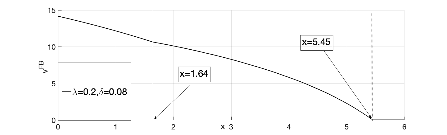
To determine the domain $[0,x_{max}]$ on which the Principal proposes a contract to the Agent (that we call simply the continuation region by analogy with the second best-case), we compute first $\lambda_{Lag}(x)$ solution of (5.1), then $H_{s}(x)=\varphi(A_{s}(x))-R_{s}(x),$ and finally $\int_{0}^{\infty}e^{-\delta s}H_{s}(x)ds$ . As $x\rightarrow H_{s}(x)$ is decreasing, $x_{max}$ is the solution $\int_{0}^{\infty}e^{-\delta s}H_{s}(x)ds=0$ : if the Agent’s reservation value is greater than $x_{max}$ , then the Principal’s value function would be negative if he proposes such a contract to the Agent. We find that the continuation region is equal to $[0,5.45]$ (see Figure 4).
Figure 3 represents the variation of the Lagrange multiplier as a function of $x$ . We recall that on $[0,3\frac{\alpha}{\beta}]$ , $\lambda_{Lag}$ is solution to

\dfrac{c}{(pc\lambda_{Lag})^{\frac{p}{p-1}}(\lambda-\frac{p}{p-1}(\lambda-\delta))}+\frac{1}{\lambda}-\left(\frac{3\alpha}{\beta\lambda_{Lag}}\right)^{\frac{\beta}{\alpha+\beta}}\dfrac{\alpha+\beta}{\lambda\alpha+\beta\delta}={x}

and on $[3\frac{\alpha}{\beta},\infty[,\lambda_{Lag}$ is solution to

\dfrac{c}{(pc\lambda_{Lag})^{\frac{p}{p-1}}(\lambda-\frac{p}{p-1}(\lambda-\delta))}+\left(\frac{1}{\lambda}\left(\frac{3\alpha}{\beta\lambda_{Lag}}\right)^{\frac{\lambda}{\lambda-\delta}}-\dfrac{\alpha+\beta}{\lambda\alpha+\beta\delta}\left(\frac{3\alpha}{\beta\lambda_{Lag}}\right)^{\frac{\lambda}{\lambda-\delta}}\right)=x.

In this numerical study $\lambda_{Lag}=3\frac{\alpha}{\beta}=3$ corresponds to $x=1.64$ .

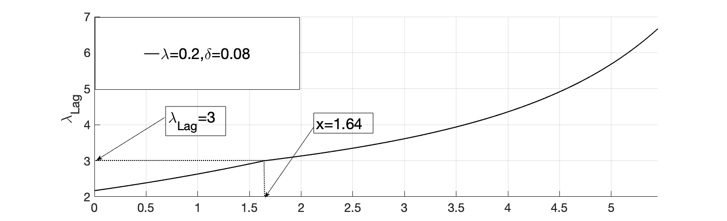
Figure 4 represents the value function for the Principal. The discontinuity in the slope of the curve at $x=1.64$ corresponds to the $x$ -value for which $\lambda_{Lag}=\frac{3\alpha}{\beta}=3.$

Figures 5 and 6 represent the optimal rent paid by the Principal, as a decreasing function of the effort provided by the Agent, for two different values of $t=0$ and $t=25$ .
Refer to caption Figure 5: Optimal rent as a function of the effort for $t=0$ (first-best case) Figure 6: Optimal rent as a function of the effort for $t=15$ (first-best case)

Figure 11 (resp. Figure 10) represents the optimal rent (resp. optimal effort) as a function of $x$ an $t$ . The optimal rent is decreasing in $t$ (since the Agent is more impatient than the Principal) and increasing in $x$ . Besides, the optimal effort is increasing in $t$ and decreasing in $x$ .

Figures 9, 11 and 10 below provide a focus of the value function and optimal effort/rent on a smaller interval $x\in[0,0.95]$ to stay on a similar interval than in the second-best case (see the continuation region in the second-best case in Section 5.2).

5.2 Second-best case

We approximate numerically the solution of the HJBVI (4.28) by using a policy iteration algorithm named Howard algorithm. The numerical approximation of the solution of (4.28) consists in three steps (for more details see Hajjej et al. [HHM22]):

1.

Reduction to a bounded domain. We have to replace $[0,\infty)$ by a bounded domain $[0,\overline{x}]$ . Since the behavior of the HJB solution at $\infty$ is known, $v(x)=-U^{-1}(x)$ for $x$ large enough, and we take this boundary condition. The choice of the boundary $\overline{x}$ is empirical and the robustness is studied by varying $\overline{x}$ .
2.

We use finite difference approximations to discretize the variational inequality (4.28).
3.

We use Howard algorithm (see Howard [How60]) to solve the discrete equation.

In this section we use the same functions $\varphi,h$ and $U$ as in the first-best case. We first take the following value for the volatility $\sigma=1.85$ . We observe in Figures 12 and 13 that the value function is concave, in accordance with Sannikov [San08]. The continuation region is (0, 0.32) on which the value function is strictly concave, then it is equal to $-U^{-1}(x)$ .

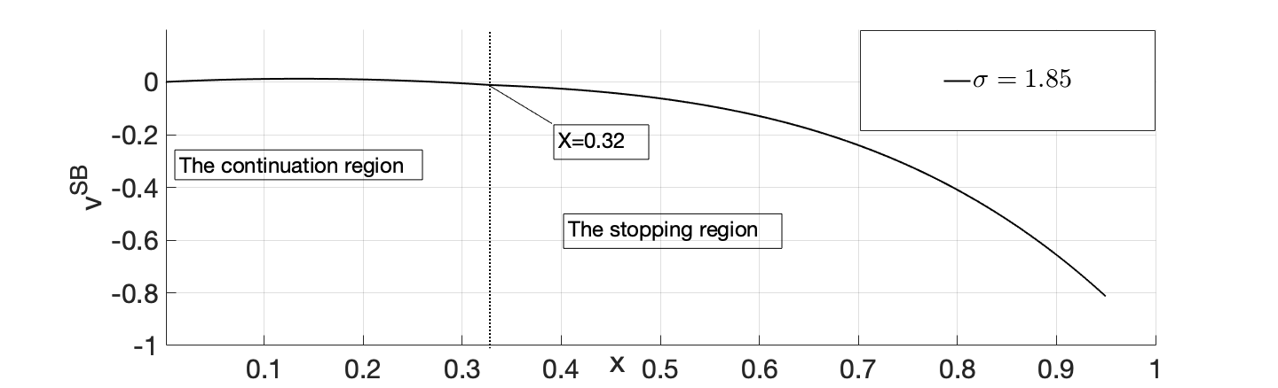
Figure 14 computes the value function for different value of $\sigma$ . The higher $\sigma$ , the smaller the value function for the Principal. These numerical results are in accordance with the ones obtained in [HHM22] established in a weak approach.

5.3 The value of the information

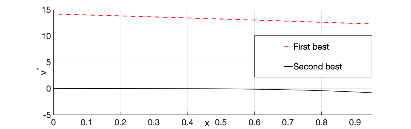
Let us first compare the optimal effort (Figures 15-16-17) and the optimal rent (Figures 18-19-20) in the first-best and second-best cases. For both cases, the higher is $x$ the reservation value for the Agent, the fewer effort the Agent will provide, and the higher the rent he will receive. Roughly speaking, when the Agent is richer, he is less motivated to provide effort, and the Principal should pay him more to prompt him to give more effort. If we focus on the first-best case, Figures 15 and 18 correspond to the optimal effort and optimal rent at time $t=0$ : since the Agent is more impatient than the Public, the Principal agrees to pay a higher rent and to receive a lower effort from the Agent at the beginning of the contract, compared to second-best case. As shown in the previous Figures 10 and 11, as well as in Figures 16 and 19, the rent will then rapidly decrease in time, and the effort will increase. In addition the contract in the first-best case is perpetual, while it may stop at a stopping time in the second best case, such that the first-best case is ultimately much more favorable for the Principal than the second-best case, as shown in Figure 21.

Let us now compare in Figure 21 the Principal value function in the first-best and in the second-best cases. As the Principal is risk-neutral, the difference represents the "value of information", computed in Figure 22. The value function for the Principal in the first-best case is greater than the value function for the Principal in the second-best case. The continuation region in the first-best case ( $[0,5.45]$ ) is much larger than in the second-best ( $[0,0.32]$ ), thanks to the risk sharing between the Principal and Agent. The value function in the first-best case is equal to zero in the stopping region ( $\tau=0$ is optimal), but in second-best case the value function in the stopping region is negative equal to $-U^{-1}(x)$ . We focus below on the region $x\in[0,0.95]$ . The value of the information is a convex function of $x$ . This, together with Figure 14, shows the higher the risk, the more the value of the information.

6 Appendix

Proof of Theorem 4.8

$[(a)]$ First step: We prove $v^{aux}\geq w$ on $\mathbb{R}^{+}$ . Let $x\geq 0$ , $n\in\mathbb{N},$ and an admissible contract $(R,\tau,A^{*}(Z))\in\mathcal{G}$ . If $x=0$ , then from assumption(i), we have $v(0)=w(0)=0$ . We assume that $0<x$ . We introduce the following $\mathbb{F}$ -stopping time:

\tau_{n}~:=~\tau\wedge\inf\{t:|w^{\prime}(J_{t}^{Ag}(x,R,\tau,A^{*}(Z))){\sigma\frac{h^{\prime}(A^{*}(Z_{t}))}{\varphi^{\prime}(A^{*}(Z_{t}))}}|>n\}.

From (i)-(ii), $w$ is continuous on $\mathbb{R}_{+}$ , $w\in C^{2}([0,\hat{b}))$ and $w=-U^{-1}\in C^{2}([\hat{b},\infty))$ , then $w$ is continuous and piecewise $C^{2}$ on $\mathbb{R}_{+}$ . Applying the generalized Itô’s formula (see Krylov [Kry08], Theorem 2, p. 124) between time $0$ en $\tau_{n}$ to the process $\left(e^{-\delta t}w(J_{t}^{Ag}(x,R,\tau,A^{*}(Z)))\right)_{t\geq 0}$

	$\displaystyle w(x)$	$\displaystyle=$	$\displaystyle e^{-\delta\tau_{n}}w(J_{\tau_{n}}^{Ag}(x,R,\tau,A^{}(Z)))-\int_{0}^{\tau_{n}}e^{-\delta s}[-\delta w(J_{s}^{Ag}(x,R,\tau,A^{}(Z)))$
		$\displaystyle+$	$\displaystyle{\cal{L}}^{A^{}(Z_{s}),R_{s}}w(J_{s}^{Ag}(x,R,\tau,A^{}(Z)))]ds+\int_{0}^{\tau_{n}}e^{-\delta s}w^{\prime}(J_{s}^{Ag}(x,R,\tau,A^{}(Z)))\sigma\frac{h^{\prime}(A^{}(Z_{s}))}{\varphi^{\prime}(A^{}(Z_{s}))}{{\mathbf{1}}_{\{A^{}(Z_{s})>0\}}}dW_{s}.$

Taking the expectation, we obtain:

$\displaystyle w(x)$	$\displaystyle=$	$\displaystyle\mathbb{E}\Bigg[e^{-\delta\tau_{n}}w(J_{\tau_{n}}^{Ag}(x,R,\tau,A^{}(Z)))-\int_{0}^{\tau_{n}}e^{-\delta s}[-\delta w(J_{s}^{Ag}(x,R,\tau,A^{}(Z)))$	(6.1)
	$\displaystyle+$	$\displaystyle{\cal{L}}^{A^{}(Z_{s}),R_{s}}w(J_{s}^{Ag}(x,R,\tau,A^{}(Z)))]ds\Bigg]$
	$\displaystyle\geq$	$\displaystyle\mathbb{E}\left[e^{-\delta\tau_{n}}w(J_{\tau_{n}}^{Ag}(x,R,\tau,A^{}(Z)))+\int_{0}^{\tau_{n}}e^{-\delta s}(\varphi(A^{}(Z_{s}))-R_{s})ds\right],$

where the inequality is obtained by using assumptions(iii)-(iv).
By using the definition of the set $\mathcal{D}^{Ag}_{\rho}$ , and Cauchy Schwarz inequality, we have

\displaystyle\sup_{n\in\mathbb{N}}\mathbb{E}\big[\int_{0}^{\tau_{n}}e^{-\delta s}(\varphi(A^{*}(Z_{s}))-R_{s})ds\big]\leq\frac{1}{\delta}\mathbb{E}\big[\int_{0}^{\infty}e^{-\delta s}|\varphi(A^{*}(Z_{s}))|^{2}+|R_{s}|^{2}ds\big]<\infty.

Therefore, $\displaystyle\sup_{n\in\mathbb{N}}\mathbb{E}\big[\int_{0}^{\tau_{n}}e^{-\delta s}(\varphi(A^{*}(Z_{s}))-R_{s})ds\big]<\infty$ , so we have $(\int_{0}^{\tau_{n}}e^{-\delta s}\varphi(A^{*}(Z_{s})-R_{s})ds)_{n\in\mathbb{N}}$ is uniformly integrable. Thus, we have the convergence in $\mathbb{L}^{1}$ and we may pass to the limit as $n\rightarrow\infty$ , and we get

\displaystyle\lim_{n\rightarrow\infty}\mathbb{E}[\int_{0}^{\tau_{n}}e^{-\delta s}(\varphi(A^{*}(Z_{s}))-R_{s})ds]=\mathbb{E}[\int_{0}^{\tau}e^{-\delta s}(\varphi(A^{*}(Z_{s}))-R_{s})ds].

(6.2)

As $w$ satisfies the growth condition (4.30), we have

\displaystyle\mathbb{E}\left[|e^{-\delta\tau_{n}}w(J_{\tau_{n}}^{Ag}(x,R,\tau,A^{*}(Z)))|\right]

\displaystyle\leq

\displaystyle\mathbb{E}\left[|e^{-\delta\tau_{n}}K(1+U^{-1}(J^{Ag}_{\tau_{n}}(x,R,\tau,A^{*}(Z))))|\right]

Using (4.31), $\sup_{n\in\mathbb{N}}\mathbb{E}\left[|e^{-\delta\tau_{n}}w(J_{\tau_{n}}^{Ag}(x,R,\tau,A^{*}(Z)))|\right]<\infty$ and we may pass to the limit as $n\rightarrow\infty$ , and we get

\displaystyle\lim_{n\rightarrow\infty}\mathbb{E}[e^{-\delta\tau_{n}}w(J_{\tau_{n}}^{Ag}(x,R,\tau,A^{*}(Z)))]=E[e^{-\delta\tau}w(J_{\tau}^{Ag}(x,R,\tau,A^{*}(Z)))].

(6.3)

By (6.1), (6.2) and (6.3), we have

w(x)\geq\mathbb{E}\left[\int_{0}^{\tau}e^{-\delta s}(\varphi(A^{*}(Z_{s}))-R_{s})ds+e^{-\delta\tau}w(J_{\tau}^{Ag}(x,R,\tau,A^{*}(Z)))\right].

From assumption (ii), $w(J_{\tau}^{Ag}(x,R,\tau,A^{*}(Z)))\geq-U^{-1}(J_{\tau}^{Ag}(x,R,\tau,A^{*}(Z)))$ , and we deduce

w(x)\geq\mathbb{E}\left[\int_{0}^{\tau}e^{-\delta s}(\varphi(A^{*}(Z_{s}))-R_{s})ds-e^{-\delta\tau}J_{\tau}^{Ag}(x,R,\tau,A^{*}(Z))\right].

By taking the supremum, we obtain

w(x)\geq\displaystyle\sup_{(R,\tau,A^{*}(Z))\in{\cal{G}}}\mathbb{E}\left[\int_{0}^{\tau}e^{-\delta s}(\varphi(A^{*}(Z_{s}))-R_{s})ds-e^{-\delta\tau}J_{\tau}^{Ag}(x,R,\tau,A^{*}(Z))\right]=v^{aux}(x).

Second step: We prove $v^{aux}\leq w$ on $\mathbb{R}^{+}$ If $x\geq\hat{b}$ , then from assumption (ii) and the definition of the value function (4.26), we have $v^{aux}(x)\geq w(x)$ .
From now, we assume that $0<x<\hat{b}$ . We now consider the feedback control $(r^{*}(\widehat{J^{Ag}}),\tau^{*},a^{*}(\widehat{J^{Ag}}))$ which is assumed to be in ${\cal{G}}$ . Let $\tau^{*}$ be the stopping time introduced in (4.33). Then $\tau^{*}\in{\cal{T}}.$ We introduce the following $\mathbb{F}$ -stopping time:

\tau_{n}~:=~\tau^{*}\wedge\inf\{t:{|w^{\prime}(\widehat{J_{t}^{Ag})}}{\sigma\frac{h^{\prime}(a^{*}(\widehat{J_{t}^{Ag}})}{\varphi^{\prime}(a^{*}(\widehat{J_{t}^{Ag}})}})|>n\}.

Observe that $w(\widehat{J_{t}^{Ag}})>-U^{-1}(\widehat{J_{t}^{Ag}})$ on $[\![0,\tau_{n}{[\![}\subset[\![0,\tau^{*}[\![$ . Then on $[\![0,\tau_{n}[\![$ , by (4.28)

\delta w({\widehat{J}^{Ag}}_{t})-[{\cal L}^{a^{*}({\widehat{J}^{Ag}}_{t}),r^{*}({\widehat{J}^{Ag}}_{t})}w({\widehat{J}^{Ag}}_{t})+\varphi(a^{*}({\widehat{J}^{Ag}}_{t}))-r^{*}({\widehat{J}^{Ag}}_{t})]=0.

Therefore

	$\displaystyle w(x)$	$\displaystyle=$	$\displaystyle\mathbb{E}\left[e^{-\delta\tau_{n}}w({\widehat{J}}_{\tau_{n}}^{Ag})-\int_{0}^{\tau_{n}}e^{-\delta s}\big(-\delta w({{\widehat{J}^{Ag}}}_{s})+{\cal{L}}^{a^{}({{\widehat{J}^{Ag}}}_{s}),r^{}({\widehat{J}^{Ag}}_{s})}w({{\widehat{J}^{Ag}}}_{s})\big)ds\right]$
		$\displaystyle=$	$\displaystyle\mathbb{E}\left[e^{-\delta\tau_{n}}w({\widehat{J}^{Ag}}_{\tau_{n}})+\int_{0}^{\tau_{n}}e^{-\delta s}(\varphi(a^{}({\widehat{J}^{Ag}}_{s}))-r^{}({\widehat{J}^{Ag}}_{s}))ds\right].$

Similarly to the first step, we show that $(\int_{0}^{\tau_{n}}e^{-\delta s}(\varphi(a^{*}({\widehat{J}^{Ag}}_{s}))-r^{*}({\widehat{J}^{Ag}}_{s}))ds)_{n}$ and $\left(w(\widehat{J^{Ag}_{\tau_{n}}})\right)_{n}$ are uniformly integrable. We may pass to the limit $n\rightarrow\infty$ , $\tau_{n}\rightarrow\tau^{*}$ a.s, and since $w({\widehat{J}^{Ag}}_{\tau^{*}})=-{\widehat{J}^{Ag}}_{\tau^{*}}$ , we obtain

$\displaystyle w(x)$	$\displaystyle=$	$\displaystyle\mathbb{E}\left[\int_{0}^{\tau^{}}e^{-\delta s}(\varphi(a^{}({\widehat{J}^{Ag}}_{s}))-r^{}({\widehat{J}^{Ag}}_{s}))ds-e^{-\delta\tau^{}}{\widehat{J}^{Ag}}_{\tau^{*}}\right]$
	$\displaystyle=$	$\displaystyle J^{P}_{0}(r^{}({\widehat{J}^{Ag}}),\tau^{},a^{*}({\widehat{J}^{Ag}}))$
	$\displaystyle{\leq}$	$\displaystyle v^{aux}(x).$

We conclude that $w=v^{aux}$ on $\mathbb{R}^{+}$ and $(r^{*}({\widehat{J}^{Ag}}),\tau^{*},a^{*}({\widehat{J}^{Ag}}))$ is an optimal feedback control.
$[(b)]$ For $x\in(0,\hat{b})$ , we maximize the function

f(x,.):r\mapsto-w^{\prime}(x)U(r)-r.

When $w^{\prime}(x)\geq 0$ , the function $f(x,.)$ is non-increasing and the optimum is achieved for $r=0.$
Otherwise, the function $f(x,.)$ is concave and the optimal rent is given by $r^{*}(x)=\argmax_{r}(f(x,r)).$ Therefore $r^{*}(x)=(U^{\prime})^{-1}(\frac{-1}{w^{\prime}(x)}){\mathbf{1}}_{w^{\prime}(x)<0}.$

References

[ABS03] Jürgen Amendinger, Dirk Becherer, and Martin Schweizer. A monetary value for initial information in portfolio optimization. Finance and Stochastics, 7(1):29–46, 2003.
[AEÉ⁺20] Clémence Alasseur, Ivar Ekeland, Romuald Élie, Nicolás Hernández Santibáñez, and Dylan Possamaï. An adverse selection approach to power pricing. SIAM Journal on Control and Optimization, 58(2):686–713, 2020.
[AP13] Emmanuelle Auriol and Pierre M Picard. A theory of bot concession contracts. Journal of Economic Behavior & Organization, 89:187–209, 2013.
[APT22] René Aïd, Dylan Possamaï, and Nizar Touzi. Optimal electricity demand response contracting with responsiveness incentives. Mathematics of Operations Research, 2022.
[Arr64] Kenneth J Arrow. The role of securities in the optimal allocation of risk-bearing. The Review of Economic Studies, 31(2):91–96, 1964.
[Bel57] RE Bellman. Dynamic programming, Princeton university press, 1957.
[Ben04] Alain Bensoussan. Stochastic Control of Partially Observable Systems. Cambridge University Press, 2004.
[Bor92] Karl Borch. Equilibrium in a reinsurance market. In Foundations of Insurance Economics, pages 230–250. Springer, 1992.
[CCZ07] Abel Cadenillas, Jakša Cvitanić, and Fernando Zapatero. Optimal risk-sharing with effort and project choice. Journal of Economic Theory, 133(1):403–440, 2007.
[CET07] Guillaume Carlier, Ivar Ekeland, and Nizar Touzi. Optimal derivatives design for mean–variance agents under adverse selection. Mathematics and Financial Economics, 1(1):57–80, 2007.
[CPT17] Jakša Cvitanić, Dylan Possamaï, and Nizar Touzi. Moral hazard in dynamic risk management. Management Science, 63(10):3328–3346, 2017.
[CWZ04] Jakša Cvitanic, Xuhu Wan, and Jianfeng Zhang. First-best contracts for continuous-time principal-agent problems. Journal of Applied Mathematics and Stochastic Analysis, 2004.
[CZ12] Jakša Cvitanic and Jianfeng Zhang. Contract Theory in Continuous-Time Models. Springer Science & Business Media, 2012.
[EMRT21] Omar El Euch, Thibaut Mastrolia, Mathieu Rosenbaum, and Nizar Touzi. Optimal make–take fees for market making regulation. Mathematical Finance, 31(1):109–148, 2021.
[HHM22] Ishak Hajjej, Caroline Hillairet, and Mohamed Mnif. Optimal stopping contract for public private partnerships under moral hazard. Frontiers of Mathematical Finance, 1(4):539–573, 2022.
[HHMP17] Ishak Hajjej, Caroline Hillairet, Mohamed Mnif, and Monique Pontier. Optimal contract with moral hazard for public private partnerships. Stochastics, 89(6-7):1015–1038, 2017.
[HM87] Bengt Holmstrom and Paul Milgrom. Aggregation and linearity in the provision of intertemporal incentives. Econometrica: Journal of the Econometric Society, 55(2):303–328, 1987.
[How60] Ronald A Howard. Dynamic programming and Markov processes. John Wiley, 1960.
[Kry08] Nikolaj Vladimirovič Krylov. Controlled diffusion processes, volume 14. Springer Science & Business Media, 2008.
[MP18] Thibaut Mastrolia and Dylan Possamaï. Moral hazard under ambiguity. Journal of Optimization Theory and Applications, 179(2):452–500, 2018.
[Mül97] Holger M Müller. The first-best sharing rule in the continuous-time principal-agent problem with exponential utility. 1997.
[San08] Yuliy Sannikov. A continuous-time version of the principal-agent problem. The Review of Economic Studies, 75(3):957–984, 2008.
[SS93] Heinz Schättler and Jaeyoung Sung. The first-order approach to the continuous-time principal–agent problem with exponential utility. Journal of Economic Theory, 61(2):331–371, 1993.
[Sun05] Jaeyoung Sung. Optimal contracts under adverse selection and moral hazard: a continuous-time approach. The Review of Financial Studies, 18(3):1021–1073, 2005.
[Wil68] Robert Wilson. The theory of syndicates. Econometrica: journal of the Econometric Society, pages 119–132, 1968.

$\displaystyle{\cal{G}^{X}}$	$\displaystyle:=$	$\displaystyle\{(R,\tau,A^{}(Z))~R\geq 0~{\mathbb{F}}^{X}\mbox{-progressively measurable},\tau\in{\cal{T}^{X}},{A^{}(Z)}\geq 0~{\mathbb{F}}^{X}\mbox{-progressively}$
		$\displaystyle\mbox{ measurable such that}~\mathbb{E}\left[\int_{0}^{\infty}e^{(\rho-2\delta)s}\|\varphi(A^{*}(Z_{s}))\|^{2}ds\right]<\infty,\,\,\mathbb{E}\left[\int_{0}^{\infty}e^{(\rho-2\delta)s}\|R_{s}\|^{2}ds\right]<\infty,$
		$\displaystyle\mbox{ and }\mathbb{E}\left[e^{(\rho-2\delta)s}\|U^{-1}(J_{\tau}^{Ag}(x,R,\tau,A^{*}(Z)))\|^{2}{\mathbf{1}}_{\{\tau<\infty\}}\right]<\infty\}.$

$\displaystyle{\cal{G}}$	$\displaystyle:=$	$\displaystyle\{(R,\tau,A^{}(Z))~R\geq 0~{\mathbb{F}}\mbox{-progressively measurable},\tau\in{\cal{T}},{A^{}(Z)}\geq 0~{\mathbb{F}}\mbox{-progressively}$
		$\displaystyle\mbox{ measurable such that}~\mathbb{E}\left[\int_{0}^{\infty}e^{(\rho-2\delta)s}\|\varphi(A^{*}(Z_{s}))\|^{2}ds\right]<\infty,\,\,\mathbb{E}\left[\int_{0}^{\infty}e^{(\rho-2\delta)s}\|R_{s}\|^{2}ds\right]<\infty,$
		$\displaystyle\mbox{ and }\mathbb{E}\left[e^{(\rho-2\delta)s}\|U^{-1}(J_{\tau}^{Ag}(x,R,\tau,A^{*}(Z)))\|^{2}{\mathbf{1}}_{\{\tau<\infty\}}\right]<\infty\}.$