\proglangPStrata: An \proglangR Package for Principal Stratification

Bo Liu
Duke University Fan Li
Duke University Email: bo.liu1997@duke.edu Email: fl35@duke.edu

\Plaintitle

PStrata: Principal Stratification in R \ShorttitlePStrata: Principal Stratification in \proglangR \AbstractPost-treatment confounding is a common problem in causal inference, including special cases of noncompliance, truncation by death, surrogate endpoint, etc. Principal stratification (Frangakis and Rubin 2002) is a general framework for defining and estimating causal effects in the presence of post-treatment confounding. A prominent special case is the instrumental variable approach to noncompliance in randomized experiments (Angrist et al. 1996). Despite its versatility, principal stratification is not accessible to the vast majority of applied researchers because its inherent latent mixture structure requires complex inference tools and highly customized programming. We develop the \proglangR package \pkgPStrata to automatize statistical analysis of principal stratification for several common scenarios. \pkgPStrata supports both Bayesian and frequentist paradigms. For the Bayesian paradigm, the computing architecture combines R, C++, Stan, where R provides user-interface, Stan automatizes posterior sampling, and C++ bridges the two by automatically generating Stan code. For the Frequentist paradigm, \pkgPStrata implements a triply-robust weighting estimator. \pkgPStrata accommodates regular outcomes and time-to-event outcomes with both unstructured and clustered data. \KeywordsCausal inference, Compliers average causal effect, Instrumental variable, Principal stratification, Noncompliance, Truncation-by-death, Stan \PlainkeywordsJSS, style guide, comma-separated, not capitalized, R \AddressBo Liu, Fan Li
Department of Statistical Science
Duke University
Box 90251
Durham, NC 27705, United States of America
E-mail: ,

1 Introduction

Post-treatment confounding is a common problem in causal inference. Special cases include but not limited to noncompliance in randomized experiments, truncation by death, surrogate endpoint, treatment switching, and recruitment bias in cluster randomized trials. Principal stratification (PS) (Frangakis and Rubin 2002) is a general framework for defining and estimating causal effects in the presence of post-treatment confounding. The instrumental variable approach to noncompliance in randomized experiments (Angrist et al. 1996) can be viewed as a special example of PS. Despite its versatility, PS is not accessible to most domain scientists because it requires complex modeling and inference tools such as mixture models and highly customized programming. We develop the \proglangR package \pkgPStrata to automatize statistical analysis of several most common scenarios of PS. \pkgPStrata supports both Bayesian and Frequentist inferential strategies. For Bayesian inference, \pkgPStrata’s computing architecture combines R, C++, Stan, where R provides user-interface, Stan automatizes posterior sampling, and C++ bridges the two by automatically generating corresponding Stan code. For Frequentist inference, \pkgPStrata implements a triply-robust weighting estimator jiang2022. \pkgPStrata accommodates regular outcomes and time-to-event outcomes with both unstructured and clustered data.

This article reviews and illustrates the \pkgPStrata package. In Section 2, we review the statistical framework of PS and its several most common special cases. Section 3 describes the main functions in \pkgPStrata. Section 4 illustrates these functions with two simulated examples on noncompliance with both continuous and time-to-event outcomes.

2 Overview of Principal Stratification

Before diving into the details of \pkgPStrata, we briefly introduce the basics of the PS framework. Post-treatment confounded variables lie on the causal pathway between the treatment and the outcome; they are potentially affected by the treatment and also affect the response. Since the landmark papers by Angrist et al. 1996 and Frangakis and Rubin 2002, a large literature on this topic has been developed. The post-treatment variable setting includes a wide range of specific examples, such as noncompliance (Imbens and Rubin 1997, e.g.), outcomes censored due to death (Rubin 2006; Zhang et al. 2009, e.g.), surrogate endpoints (Gilbert and Hudgens 2008; Jiang et al. 2016, e.g.). Below we first review the framework in the context of noncompliance in randomized experiments.

For unit $i\ (i=1,\ldots,N)$ in an iid sample from a population, let $Z_{i}$ be the treatment assigned to ( $1$ for treatment and $0$ for control), and $D_{i}$ be the treatment received ( $1$ for treatment and $0$ for control). When $Z_{i}\neq D_{i}$ , noncompliance occurs. Because $D$ occurs post assignment, it has two potential values, $D_{i}(0)$ and $D_{i}(1)$ , with $D_{i}=D_{i}(Z_{i})$ . The outcome $Y_{i}$ also has two potential outcomes, $Y_{i}(0)$ and $Y_{i}(1)$ . Angrist et al. 1996 classified the units into four compliance types based on their joint potential status of the actual treatment, $S_{i}=(D_{i}(1),D_{i}(0))$ : compliers $S_{i}=(1,0)=\textup{co}$ , never-takers $S_{i}=(0,0)=\textup{nt}$ , always-takers $S_{i}=(1,1)=\textup{at}$ , and defiers $S_{i}=(0,1)=\textup{df}$ . This classification is later generalized to principal stratification (Frangakis and Rubin 2002) and the compliance types are special cases of principal strata.

The key property of principal strata $S_{i}$ is that they are not affected by the treatment assignment, and thus can be regarded as a pre-treatment variable. Therefore, comparisons of $Y_{i}(1)$ and $Y_{i}(0)$ within a principal stratum—the principal causal effects (PCEs)—have a causal interpretation:

\tau_{u}=\bE\{Y_{i}(1)-Y_{i}(0)\mid S_{i}=s\}=\bE\{Y_{i}(1)\mid S_{i}=s\}-\bE\{Y_{i}(0)\mid S_{i}=s\},

for $u=\textup{nt},\textup{co},\textup{at},\textup{df}$ . The conventional causal estimand in the noncompliance setting is the intention-to-treat (ITT) effect, which is equivalent to the average causal effect of the assignment (ATE) and can be decomposed into the sum of the four PCEs:

\textsc{ITT}=\bE\{Y_{i}(1)-Y_{i}(0)\}=\sum_{s}\pi_{s}\tau_{s},

where $\pi_{s}=\Pr(S_{i}=s)$ is the proportion of the stratum $s$ .

2.1 Randomized Experiments with Noncompliance

Due to the fundamental problem of causal inference, individual compliance stratum $S_{i}$ is not observed. Therefore, additional assumptions are required to identify the stratum-specific effects. Besides randomization of $Z_{i}$ , Angrist et al. 1996 make two additional assumptions.

Assumption 1.

(Monotonicity): $D(1)\geq D(0)$ , i.e. there is no $10$ or defiers stratum.

Under monotonicity, there are only two strata–never-takers and compliers—in the one-sided noncompliance setting (i.e. control units have no access to treatment), and three strata—never-takers, compliers and always-takers—in the two-sided noncompliance setting (i.e. control units also have access to treatment).

Assumption 2.

(Exclusion restriction): for stratum $s$ in which $D(0)=D(1)$ , i.e., $s=00,11$ , $E[Y_{i}(1)-Y_{i}(0)|S_{i}=s]=0$ .

In the context of noncompliance, exclusion restriction states that for never-takers and always-takers, the causal effects of the assignment $Z$ is 0. Exclusion restriction rules out the direct effect from the assigned treatment to the outcome, no mediated through the actual treatment.

Under monotonicity and exclusion restriction, the complier average causal effect is nonparametrically identifiable as

\tau_{\textup{co}}\equiv\bE\{Y(1)-Y(0)\mid S=\textup{co}\}=\frac{\bE(Y\mid Z=1)-\bE(Y\mid Z=0)}{\bE(D\mid Z=1)-\bE(D\mid Z=0)},

which is exactly the probability limit of the two-stage least squares estimator Angrist et al. 1996. Because under monotonicity, only compliers’ actual treatments are affected by the assignment, $\tau_{\textup{co}}$ can be interpreted as the effect of the treatment.

2.2 Truncation by Death

“Truncation by death” is a case where the outcome is not defined on some units whose intermediate variable is of certain value. The name comes from an original example, where treatment $Z$ is a medical invention, outcome $Y$ is quality of life at the end of the study, and $D$ is the survival status of the patient at the end of the study. Arguably quality of life is only defined for patients who are alive, and thus the outcome is “truncated or censored by death" for patients who died. Rubin 2006 proposed to use Principal Stratification to address truncation by death. Here the four strata are sometimes named as “never-survivor”, “always-survivor”, “compliers” and “defiers”. Treatment effect is well-defined only in the “always-survivor” stratum, and is called “survivor average causal effect (SACE)”. Monotonicity is usually still plausible, but exclusion restriction no longer applies. various another assumptions have been proposed in the literature.

2.3 Model-based analysis of PS

We now describe the Bayesian inference of the IV setup, first outlined in Imbens and Rubin 1997. Without any assumption, the observed cells of $Z$ and $D$ consist of a mixture of units from more than one stratum. For example, the units who are assigned to the treatment arm and took the treatment ( $Z=1,D=1$ ) can be either always-takers or compliers. One has to disentangle the causal effects for different compliance types from observed data. Therefore, model-based inference here resembles that of a mixture model. In Bayesian analysis, it is natural to impute the missing label $S_{i}$ under some model assumptions. Specifically, to conduct Bayesian inference with posttreatment variables, besides the prior distribution for the parameter $\theta$ , one need to specify two models:

1.

S-model, i.e., principal strata model given covariates: $S_{i}\mid X_{i}$ ;
2.

Y-model, i.e., outcome model given stratum, covariates and treatment: $Y_{i}\mid S_{i},X_{i},Z_{i}$

A common model choice is a multinomial logistic regression for $S_{i}$ and a generalized linear model for $Y_{i}$ . We can simulate the joint posterior distribution $\Pr(\theta,\mathbf{D}^{\textup{mis}}\mid\mathbf{Y}^{\textup{obs}},\mathbf{D}^{\textup{obs}},\bm{Z},\bm{X})$ by iteratively imputing the missing $S$ from $\Pr(\mathbf{D}^{\textup{mis}}\mid\mathbf{Y}^{\textup{obs}},\mathbf{D}^{\textup{obs}},\bm{Z},\bm{X},\theta)$ and updating the posterior distribution of $\theta$ from $\Pr(\theta\mid\mathbf{Y}^{\textup{obs}},\mathbf{D}^{\textup{obs}},\mathbf{D}^{\textup{mis}},\bm{Z},\bm{X})$ . For more details, see Imbens and Rubin 1997; Hirano et al. 2000.

2.4 Frequentist approach under principal ignorability

For the frequentist approach, \pkgPStrata implements the weighting-based multiply-robust estimator in Jiang et al. 2022. The key assumption is principal ignorability (Jo and Stuart 2009).

Assumption 3.

(Principal Ignorability) $\E[Y(1)|s=11,X]=\E[Y(1)|s=10,X]$ and $E[Y(0)|s=00,X]=\E[Y(0)|s=10,X]$

Principal ignorability assumes away the mixture structure of principal stratification. Instead one can construct an inverse probability weighting based multiply-robust estimator. Three quantities are required. Define $\pi(X)=\Pr(Z=1|X)$ as the propensity score or the treatment probability, and $e_{u}(X)=\Pr(S=s|X)$ for $s=00,01,10,11$ as the principal score. Let $\pi=\E[\pi(X)]=P(Z=1)$ and $e_{s}=\E[e_{u}(X)]=\Pr(S=s)$ be the marginalized propensity score and principal score. Also define $p_{z}(X)=\Pr(W=1|Z=z,X)$ for $z=0,1$ , the probability of the intermediate variable conditional on the treatment and covariates. Under monotonicity, it is easy to see that

e_{10}(X)=p_{1}(X)-p_{0}(X),\quad e_{11}(X)=p_{0}(X),\quad e_{00}(X)=1-p_{1}(X)

and

e_{10}=p_{1}-p_{0},\quad e_{11}=p_{0},\quad e_{00}=1-p_{1}

where $p_{z}=\E[p_{z}(X)]$ . The weighting-based estimator $\hat{\tau}^{mr}$ is a product of the inverse probability of the three scores: propensity score, principal score and the probability of the intermediate variable. If any two of the three models are correctly specified, then the estimator $\hat{\tau}^{mr}$ is consistent. With principal ignorability, we still need monotonicity, but not necessarily exclusion restriction. More details are given in Jiang et al. 2022.

3 Overview of the package

The Bayesian inference consists of three main steps. First, define data generating models, which are equivalent to specifying the joint likelihood of all observed data given parameters. Also, specify the prior distribution for these parameters. Second, draw samples from the posterior distribution of these parameters, which is obtained directly from the prior distribution and likelihood function. Third, calculate quantities of interest, which are functions of the parameters, with these posterior draws.

The Bayesian component of the package \pkgPStrata is designed to follow these steps closely, which is illustrated in Figure 1. First, the user specifies the data generating models and the prior distribution of the parameters in these models. As we shall see later, these data generating models can be constructed by simply the S-model, Y-model and assumptions. Then, \pkgPStrata relies on the \pkgStan language to draw samples from the posterior distribution. With user specification of the models and the dataset, \pkgPStrata automatically generates corresponding \pkgStan code and \pkgStan data. The code and data are processed by \pkgStan to facilitate the posterior sampling process. Finally, these posterior samples are passed back to \pkgPStrata for post-process, such as calculation of estimands, summary and visualization, etc.

Figure 1: Overview of the model fitting process in \pkgPStrata

The main function in \pkgPStrata with the same name, \codePStrata, is designed to be an integrated module that bridges between the front-end and the back-end. On the front-end, users input model specification and data, and then receive posterior samples as the output. The sampling process in the back-end should be fully decoupled from the front-end so that users do not need to worry about sampling as they specify the models, which is unlikely possible for Gibbs samplers. \codePStrata incorporates two core submodules \codePSObject and \codePSSample to fulfill this requirement. The \codePSObject submodule interprets user input to generate a principal stratification object that contains essential information about model specification. The \codePSSample submodule calls \pkgStan to generate posterior samples. These posterior samples are returned in \codePStrata and can be further passed to \codePSOutcome and \codePSContrast for calculating potential outcomes and causal effects. The relationship between these modules is illustrated in Figure 2.

Figure 2: Core modules designed in \pkgPStrata. Solid arrows indicate that the start-point module is called by the end-point module. Dotted arrows indicate that the outcome of the start-point module is passed to the end-point module as an argument.

In Section x.x, we introduce the details of model specification. In Section x.x, …..

3.1 Model specification

Typical datasets used for principal stratification consist of the treatment $Z$ , the post-treatment covariate $D$ , the outcome $Y$ and covariates $X$ . To better convey to main idea, we assume that both $Z$ and $D$ are binary variables, but the idea can be readily extended to the case of non-binary but discrete $Z$ and $D$ , and the case of multiple post-treatment covariates (when $D$ is a vector). Since $D$ is observed after treatment, controlling $D$ leads to biased estimation of the causal effect, as it breaks randomization on the treatment $Z$ . However, the principal stratum $S$ , defined by the potential values of $D$ under each treatment, can be viewed as a pre-treatment variable (Imbens and Rubin 1997). When the principal stratum $S$ is fixed, no variables lie on the causal pathway from $Z$ to $Y$ ; thus the stratum-specific causal effect can be correctly estimated (Figure 3).

Figure 3: Graph illustration of principal stratification. The left panel shows that post-treatment covariate

D

lies between the causal pathway from treatment

Z

to outcome

Y

. The right panel shows that the unobservable principal stratum

S

separates

D

from the causal pathway from

Z

Y

If the principal stratum $S$ were known, the Y-model $\Pr(Y\mid X,Z,S)$ would be sufficient to estimate any causal estimand. However, as $S$ is defined as the potential values of $D$ , only one realization of them can be observed. Hence, a model for principal stratum $\Pr(S\mid X)$ is necessary to estimate $S$ . Let $\mathcal{S}$ denote the set of all possible principal strata. The data generation process can be expressed as follows.

	$\displaystyle\Pr(Z,D,Y\mid X)$	$\displaystyle=\sum_{s\in\mathcal{S}}\Pr(Z\mid X)\Pr(S=s\mid Z,X)\Pr(D\mid S=s,Z,X)\Pr(Y\mid D,S=s,Z,X)$		(3.1)
		$\displaystyle\propto\sum_{s\in\mathcal{S}:D=D(s,Z)}\Pr(S=s\mid X)\Pr(Y\mid S=s,Z,X).$		(3.2)

The first term $\Pr(Z\mid X)$ in (3.1) is a constant for randomized trials. The third term $\Pr(D\mid S=s,Z,X)$ is deterministic, and controls the set of principal strata over which the summation is taken. $D$ in the last term $\Pr(Y\mid D,S=s,Z,X)$ drops out as it has no additional information given $Z$ and $S$ .

It is shown in (3.2) that the data generating model can be expressed as a mixture model involving only the S-model and Y-model, and our aim is to disentangle such mixture from the observed data. Depending on the real application, we may impose additional assumptions to help identify the components in the mixture model. The first assumption is monotonicity which rules out defiers. In some cases when the treatment cannot be accessed by the control group, we may also rule out always-takers. In general, this assumption defines the set $\mathcal{S}$ of all strata that we include in (3.1). The second assumption is the exclusion-restriction (ER). By assuming ER for stratum $s$ , we exclude the direct causal pathway from $Z$ to $Y$ given $S$ , and consequently,

\Pr(Y\mid S=s,Z=z_{1},X)=\Pr(Y\mid S=s,Z=z_{2},X),\quad\text{if $D(s,z_{1})=D(s,z_{2})$}.

(3.3)

\pkg

PStrata offers the \codePSObject function to specify the S-model and Y-model, put assumptions on monotonicity and ER, and impose prior distributions on parameters that appear in the models. The function has the following declaration: {Code} PSObject(S.formula, Y.formula, Y.family, data, strata, ER, + prior_intercept, prior_coefficient, prior_sigma, + prior_alpha, prior_lambda, prior_theta, survival.time.points)

We will discuss in detail these arguments in subsequent sections, with the exception of \codedata and \codesurvival.time.points. The \codedata argument simply provides the dataset to fit the model. The \codesurvival.time.points argument is only used for survival models, which will be discussed later in Section x.x.

3.1.1 S-model and Y-model

In \pkgPStrata, we specify the S-model $p(S_{i}\mid X_{i})$ as a multinomial model,

\Pr(S_{i}=s\mid X_{i};\{\beta_{s}\})\propto\exp(X_{i}^{\prime}\beta_{s}).

(3.4)

When an intercept is included in the model, the $X_{i}$ in (3.4) can be understood as an augmented vector with the constant 1. To assure identifiability, a reference stratum $s_{0}\in\mathcal{S}$ is chosen and $\beta_{s_{0}}$ is fixed to zero. The S-model is equivalently expressed by

\Pr(S_{i}=s\mid X_{i};\{\beta_{s}\})=\frac{\exp(X_{i}^{\prime}\beta_{s})}{\sum_{s^{\prime}\in\mathcal{S}}\exp(X_{i}^{\prime}\beta_{s^{\prime}})}.

(3.5)

We specify the Y-model as a generalized linear model, which is flexible enough in modeling various types of data. The Y-model can be mathematically written as

Y_{i}\mid S_{i}=s,X_{i},Z_{i}=z\sim F(\mu_{sz}(X_{i}),\theta_{sz}),\\

(3.6)

where $F$ is a distribution often referred to as the family of the generalized linear model. The mean of this distribution is related to the linear combination of $X_{i}$ via a link function $g$ :

\mu_{sz}(X_{i}):=\E[Y_{i}\mid S_{i}=s,X_{i},Z_{i}=z,\gamma_{sz}]=g^{-1}(X_{i}^{\prime}\gamma_{sz}),

(3.7)

where $\{\gamma_{sz}\}$ are parameters to be estimated. Some family $F$ may have additional parameters apart from the mean, such as the standard deviation parameter in Gaussian models and the shape parameter in Gamma and inverse Gaussian models. When these parameters exists, we assume they are independent of the covariates. However, we allow these parameters to depend on the stratum $s$ and treatment $z$ , as denoted by $\theta_{sz}$ in (3.6).

The S-model and Y-model are specified with arguments \codeS.formula, \codeY.formula and \codeY.family. An (incomplete) example is given as follows. {Code} … S.formula = Z + D X, Y.formula = Y X, Y.family = binomial(link = "logit"), …

The terms before the \code symbol defines the variables essential to the pricipal stratification model. Specifically, \codeS.formula defines the treatment variable $Z$ and the post-treatment covariate $D$ concatenated by the \code+ sign, and \codeY.formula defines the response variable $Y$ . When multiple post-treatment covariates exists, they can be concatenated in order like \codeS.formula = Z + D1 + D2 X. However, we do not allow multiple treatment variables to avoid ambiguity. In cases where multiple treatment variables exists, they might be recoded into a single variable with multiple treatment arms.

The terms after the \code symbol defines the covariates that are included in (3.4) and (3.7), with the syntax exactly matching that of \codelm(). To recall the basic syntax, predictors are separated by \code+ as in \codeY X1 + X2. By default, the intercept term is included; either \codeY X1 + X2 + 0 or \codeY X1 + X2 - 1 removes the intercept. Each predictor can be a raw covariate (e.g. \codeX1), a transformed covariate (e.g. \codeI(X1ˆ2)) or the interaction of multiple covariates (e.g. \codeX1:X2).

The \codeY.family argument specifies the family and link of the generalized linear model following the convention of \codeglm(). The families and link functions supported in \pkgPStrata are listed in Table 1.

Family	Link Functions	$f(y;\mu,\theta)$
\codegaussian	\codeidentity, \codelog, \codeinverse	$\frac{1}{\sqrt{2\pi\sigma^{2}}}\exp\left(-\frac{-(y-\mu)^{2}}{2\sigma^{2}}\right)$
\codebinomial	\codelogit, \codeprobit, \codecauchit, \codelog, \codecloglog	$\mu^{y}(1-\mu)^{1-y}$
\codeGamma	\codeidentity, \codelog, \codeinverse	$\frac{(\alpha/\mu)^{\alpha}}{\Gamma(\alpha)}y^{\alpha-1}\exp(-\frac{\alpha y}{\mu})$
\codepoisson	\codeidentity, \codelog, \codesqrt	$\mu^{y}e^{-\mu}/(y!)$
\codeinverse.gaussian	\code1/muˆ2, \codeinverse, \codeidentity, \codelog	$\sqrt{\frac{\lambda}{2\pi y^{3}}}\exp\left(-\frac{\lambda(y-\mu)^{2}}{2y\mu^{2}}\right)$

Table 1: Supported families, link functions and corresponding density/mass functions expressed by the mean

\mu

and additional parameter

\theta

3.1.2 Assumptions

In the context of binary non-compliance, there are two important assumptions: monotonicity (Assumption 1) and exclusion restriction (Assumption 2). Monitonicity rules out the existence of defiers and thus all strata to be considered are always-takers, never-takers, and compliers. This can be specified by \codestrata = c(at = "11", nt = "00", co = "01"). The exclusion restriction (ER) assumes away direct effects of $Z$ on $Y$ not through $D$ for certain strata, which is specified by a binary logical vector with the same length as \codestrata, indicating whether ER is assumed for each stratum. For example, \codeER = c(True, True, False) assumes ER for both the always-takers and the never-takers, but not for the compliers. For simplicity, we introduce a short-hand specification for both assumptions by adding an asterisk (\code*) after the group where ER is assumed. As an example, the assumptions mentioned above can be specified by \codestrata = c(at = "11*", nt = "00*", co = "01"), and the \codeER argument can be left blank.

When multiple intermediate variables exist, the principal strata are defined by the potential values of each intermediate variable. To specify such a stratum, use \code| to separate the potential values of each intermediate variable. For example, the principal stratum defined by two intermediate variables $D_{1}(0)=D_{1}(1)=0$ and $D_{2}(0)=D_{2}(1)=1$ can be represented by \code"00|11".

3.1.3 Priors

The S-model and Y-model are both parametric models. These parameters include intercepts ( $\alpha_{s}$ and $\gamma_{sz}$ ), coefficients ( $\beta_{s}$ and $\eta_{sz}$ ), and other parameters specific to the family of the Y-model. As Table 1 shows, the \codegaussian family introduces a parameter $\sigma$ that represents the standard deviation of the error, the \codeGamma family introduces the shape parameter $\alpha$ , and the \codeinverse.gaussian family introduces the shape parameter $\lambda$ . We refer to these parameters as \codesigma, \codealpha and \codelambda acoording to convention.

\pkg

PStrata provides flexibility on the specification of prior distribution on these parameters, including the intercept, coefficients and model-specific parameters. The prior distribution of intercepts and coefficients can be specified in \codeprior_intercept and \codeprior_coefficient respectively. When additional parameters exists in Y-model, the prior distributions of such variables are defined by \codeprior_sigma, \codeprior_alpha or \codeprior_lambda, according to the name of the additional parameter. The full list of supported prior distributions is provided in Table 2.

By default, \codeprior_intercept is a flat (improper) distribution over the whole real line, \codeprior_coefficient is a standard gaussian distribution $\mathcal{N}(0,1)$ , and \codeprior_sigma, \codeprior_alpha and \codeprior_lambda are standard inverse-gamma distribution $\mathcal{IG}(1,1)$ .

Domain	Prior distribution	Specification
$(-\infty,\infty)$	Uniform (improper)	\codeprior_flat()
	Normal	\codeprior_normal(mean = 0, sigma = 1)
	Student $t$	\codeprior_t(mean = 0, sigma = 1, df = 1)
	Cauchy	\codeprior_cauchy(mean = 0, sigma = 1)
	Double exponential	\codeprior_lasso(mean = 0, sigma = 1)
	Logistic	\codeprior_logistic(mean = 0, sigma = 1)
$(0,\infty)$	Chi squared	\codeprior_chisq(df = 1)
	Inverse Chi squared	\codeprior_inv_chisq(df = 1)
	Exponential	\codeprior_exponential(beta = 1)
	Gamma	\codeprior_gamma(alpha = 1, beta = 1)
	Inverse Gamma	\codeprior_inv_gamma(alpha = 1, beta = 1)
	Weibull	\codeprior_weibull(alpha = 1, sigma = 1)

Table 2: List of prior distributions.

3.2 Other data types

3.2.1 Survival data

Survival data refer to the type of data where the outcome is subject to right censoring. Suppose each subject has a true event time $T_{i}$ and censoring time $C_{i}$ , but they cannot be observed due to censoring. The observed data are the censored event time $Y_{i}=\min\{T_{i},C_{i}\}$ and the event indicator $\delta_{i}=\mathbf{1}(T_{i}<C_{i})$ . According to the data generating process, we assume that there is an underlying distribution $p(T_{i},C_{i}\mid X_{i},S_{i},Z_{i})$ , which in turn decides the distribution of observed quantities $p(Y_{i},\delta_{i}\mid X_{i},S_{i},Z_{i})$ . When the censoring is conditionally ignorable, i.e., $T_{i}\perp\!\!\!\perp C_{i}\mid\{X_{i},S_{i},Z_{i}\}$ , it turns out that the distribution of $T_{i}$ and $C_{i}$ can be separated from the likelihood $p(Y_{i},\delta_{i}\mid X_{i},S_{i},Z_{i})$ :

	$\displaystyle p(Y_{i},\delta_{i}=1\mid X_{i},S_{i},Z_{i})$	$\displaystyle=p(T_{i}\geq Y_{i}\mid S_{i},Z_{i},X_{i})p(C_{i}=Y_{i}\mid S_{i},Z_{i},X_{i}),$		(3.8)
	$\displaystyle p(Y_{i},\delta_{i}=0\mid X_{i},S_{i},Z_{i})$	$\displaystyle=p(T_{i}=Y_{i}\mid S_{i},Z_{i},X_{i})p(C_{i}\leq Y_{i}\mid S_{i},Z_{i},X_{i}).$		(3.9)

As we usually only care out the true event time $T_{i}$ , the terms regarding the censoring time $C_{i}$ drops out from the likelihood, and only specification of the distribution for $T_{i}$ is needed.

Two widely used models for $T_{i}$ are the Cox proportional hazard model (Cox 1972) and the accelerated failure time (AFT) model (Wei 1992). The Cox proportional hazard model assumes that the hazard function should be

h(t;S_{i}=s,Z_{i}=z,X_{i})=h_{0}(t;s,z)\exp(X_{i}^{\prime}\beta_{s,z}),

(3.10)

where $h_{0}(t;s,z)$ is the baseline hazard function. In Bayesian inference, a parametric form of $h_{0}$ is desirable. A common form is the Weibull model (Abrams et al. 1996): $h_{0}(t;s,z)=\exp(\alpha_{s,z})t^{\varphi_{s,z}-1}$ , $\alpha_{s,z}\in\mathbb{R}$ , $\varphi_{s,z}>0$ , under which the the Cox model 3.10 takes the parameteric form (under reparameterization)

h(t;S_{i}=s,Z_{i}=z,X_{i})=t^{\exp(\theta_{s,z})-1}\exp(X_{i}^{\prime}\beta_{s,z}).

(3.11)

It can be then derived from the hazard function that

	$\displaystyle p(T_{i}\geq Y_{i}\mid S_{i}=s,Z_{i}=z,X_{i})$	$\displaystyle=\exp\left\{-t^{\exp(\theta_{s,z})}\exp(-\theta_{s,z}+X_{i}^{\prime}\beta_{s,z})\right\},$		(3.12)
	$\displaystyle p(T_{i}=Y_{i}\mid S_{i}=s,Z_{i}=z,X_{i})$	$\displaystyle=h(t;s,z,X_{i})p(T_{i}\geq Y_{i}\mid S_{i}=s,Z_{i}=z,X_{i}).$		(3.13)

The AFT model assumes that $\log(T_{i})=X_{i}^{\prime}\beta+\epsilon_{i}$ , where $\epsilon_{i}$ follows a given distribution. Commonly, we assume that $\epsilon_{i}\sim\mathrm{N}(0,\sigma^{2})$ . Then, it can be computed that

	$\displaystyle p(T_{i}\geq Y_{i}\mid S_{i}=s,Z_{i}=z,X_{i})$	$\displaystyle=1-\Phi\left(\frac{\log Y_{i}-X_{i}^{\prime}\beta_{s,z}}{\sigma_{s,z}}\right),$		(3.14)
	$\displaystyle p(T_{i}=Y_{i}\mid S_{i}=s,Z_{i}=z,X_{i})$	$\displaystyle=\phi\left(\frac{\log Y_{i}-X_{i}^{\prime}\beta_{s,z}}{\sigma_{s,z}}\right),$		(3.15)

where $\Phi$ and $\phi$ are respectively the cumulative density function and probability density function of standard normal distribution.

\pkg

PStrata allows fitting principal stratification models on survival data under the conditional ignorability assumption. Running models on survival data is similar to the normal data except some modification. First, one needs to include both censored event time $Y$ and the event indicator $\delta$ when specifying the Y-model. For example, \codeY.formula = Y + delta X specifies a Y-model where both \codeY and \codedelta appear on the left hand side of the formula. Second, the \codeY.family should be \codesurvival(method = "Cox") for the Weibull-Cox model or \codesurvival(method = "AFT") for the AFT model. Third, since the fitted outcome - the survival probability at time $t$ - is a continuous curve of $t$ , one needs to specify a set of time points where the survival probability is calculated. One either specify as a vector the customized time points to the parameter \codesurvival.time.points, or simply provide a positive integer indicating the number of time points, and the time points will be uniformly chosen from 0 to the 90% quantile of the observed event time.

3.2.2 Multi-level data

In previous sections, we assume that the units are independent samples from the population. In some applications, this assumption might be implausible when natural clusters exist, such as schools, hospitals and regions. For example, in a trial conducted at multiple medical centers, patients from the same medical center may have correlated outcomes. Hierarchical models are commonly used to model such data, by assuming that each cluster has a cluster-specific effect (random effect) drawn from some unknown distribution, and within each cluster, the outcome of the units follow some distribution related to the cluster-specific effect. The hierarchical structure is well-fit for Bayesian analyses, and \pkgPStrata allows specification of multi-level structure in both S-model and Y-model.

We introduce the most common setting where only one level of clusters exists, although \pkgPStrata provides flexibility to model various cluster strucures. Let $j=1,\dots,J$ denote the clusters, and let $C_{i}$ denote the cluster which subject $i$ belongs to. Additional to the individual covariates $X_{i}$ , let $V_{j}$ be cluster covariates of cluster $j$ . Assuming the random effects are additive, the multi-level S-model assumes that

\Pr(S_{i}=s\mid X_{i},V_{j},C_{i}=j)\propto\exp(X_{i}^{\prime}\beta_{s}+V_{j}^{\prime}\widetilde{\beta}_{s}+\eta_{j}),

(3.16)

where $\eta_{j}\sim\mathrm{N}(0,\sigma^{2})$ are cluster random effects. Similarly, the mean of the Y-model is specified as

\E(Y_{i}\mid Z_{i}=z,X_{i},V_{j},C_{i}=j)=g^{-1}(X_{i}^{\prime}\gamma_{sz}+V_{j}^{\prime}\widetilde{\gamma}_{sz}+\xi_{sz,j}),

(3.17)

where $\xi_{sz,j}\sim\mathrm{N}(0,\tau_{sz}^{2})$ are the cluster random effects.

\pkg

PStrata supports including these random effects when clusters exist, by specifying these effects in \codeS.formula and/or \codeY.formula with the same syntax as in \codelme4::lmer(). The syntax to include the above-mentioned additive random effects is to include a term \code(1 | C), where \codeC is the cluster id. For example, the Y-model mentioned above can be specified as \codeY.formula = Y X + V + (1 | C), where \codeC is a vector indicating the cluster id each unit belongs to.

The additive assumption for random effects can be relaxed to allow the coefficients $\beta_{s}$ , $\widetilde{\beta}_{s}$ , $\gamma_{sz}$ , $\tilde{\gamma}_{sz}$ to vary across cluster. For example, a random effect on the coefficient $\beta_{s}$ will modify the S-model as

\Pr(S_{i}=s\mid X_{i},V_{j},C_{i}=j)\propto\exp(X_{i}^{\prime}(\beta_{s}+\omega_{j})+V_{j}^{\prime}\widetilde{\beta}_{s}+\eta_{j}),

(3.18)

where both $\eta_{j}$ and $\omega_{j}$ are random effects drawn from distributions $\eta_{j}\sim\mathrm{N}(0,\sigma^{2}),\omega_{j}\sim\mathrm{N}(0,\kappa_{j}^{2})$ . In the literature, $\eta_{j}$ is commonly referred to as random intercept, and $\omega_{j}$ is commonly referred to as random slope.

In \pkgPStrata, the above model can be specified as \codeS.formula = S X + V + (X | C), where the term \code(X | C) specifies a random slope on $X$ and an (implicit) random intercept according to the cluster $C$ . To remove the implicit random intercept, one should specify the model as \codeS.formula = S X + V + (X - 1 | C) or \codeS.formula = S X + V + (X + 0 | C). More details on the syntax can be found in the documentation of \codelme4::lmer().

3.3 Outcome and contrast

\pkg

PStrata calls \pkgstan to draw samples from the posterior distribution of the parameters. These posterior samples can be used to calculate summary statistics, such as the stratum probability, stratum-specific potential outcomes and their contrasts.

For each parameter, we denote the sample drawn in each iteration by a superscript in parenthesis. For example, the samples drawn from the posterior distrbution $\alpha$ are denoted by $\alpha^{(1)},\alpha^{(2)},\dots,\alpha^{(B)}$ , where $B$ is the number of posterior draws.

3.3.1 Stratum probability

Recall the multinomial logistic S-model (3.4). In iteration $k$ , the estimated probability of unit $i$ being in stratum $s$ can be obtained by plugging in the posterior draws from that iteration,

p_{is}^{(k)}:=p(S_{i}=s\mid X_{i})=\frac{\exp(\beta_{s}^{(k)}{}^{\prime}X_{i})}{\sum_{\varsigma\in\mathcal{S}}\exp(\beta_{\varsigma}^{(k)}{}^{\prime}X_{i})}.

(3.19)

By calculating this quantity in each iteration, we obtain a sequence of estimated stratum probability $p_{is}^{(1)},\dots,p_{is}^{(B)}$ , which can be viewed as drawn from the posterior distribution of $p_{is}$ . With these posterior samples, \pkgPStrata calculates and reports the expectation, the standard deviation and the quantiles of the estimated stratum probabililty.

3.3.2 Outcome

Let $\mu_{sz}$ denote the average potential outcome for stratum $s$ under treatment $z$ which is defined as

$\displaystyle\mu_{sz}$	$\displaystyle=\E[Y(z)\mid S=s]$
	$\displaystyle=\E[\E[Y(z)\mid S=s,X]\mid S=s]$
	$\displaystyle=\int\E[Y(z)\mid S=s,X=x]\frac{\Pr(S=s\mid X=x)}{\Pr(S=s)}\mathbb{P}(\mathrm{d}x)$
	$\displaystyle=\frac{\int\E[Y(z)\mid S=s,X=x]\Pr(S=s\mid X=x)\mathbb{P}(\mathrm{d}x)}{\int\Pr(S=s\mid X=x)\mathbb{P}(\mathrm{d}x)}.$	(3.20)

To estimate such a quantity, we approximate the measure $\mathbb{P}(\mathrm{d}x)$ by the empirical distribution of $X$ in the data, and thus both integrals reduce to summation over each unit. Within the integrals, the first term $\E[Y(z)\mid S=s,X=x]$ is given by the Y-model (3.7),

\E[Y_{i}(z)\mid S_{i}=s,X_{i}]=g^{-1}(\gamma_{sz}^{\prime}X_{i}).

(3.21)

The term $\Pr(S=s\mid X=x)$ is exactly the stratum probability $p_{is}$ defined in the previous section. This suggests estimating the potential outcome $\mu_{sz}$ by

\displaystyle\mu_{sz}\approx\frac{\sum_{i=1}^{n}g^{-1}(\gamma_{sz}^{\prime}X_{i})p_{is}}{\sum_{i=1}^{n}p_{is}}.

(3.22)

By plugging in the posterior samples of the parameter $\gamma_{sz}$ and the stratum probability $p_{is}$ , we obtain posterior draws $\mu_{sz}^{(1)},\dots,\mu_{sz}^{(B)}$ , where

\displaystyle\mu_{sz}^{(k)}=\frac{\sum_{i=1}^{n}g^{-1}(\gamma_{sz}^{(k)}{}^{\prime}X_{i})p_{is}^{(k)}}{\sum_{i=1}^{n}p_{is}^{(k)}}.

(3.23)

The expectation, standard deviation and quantiles of the estimated potential outcomes can be obtained directly from these poterior draws.

3.3.3 Contrast

Many statistically meaningful estimands can be represented as contrasts of the potential outcomes. For example, the SATE for stratum $s$ is the difference between two potential outcomes:

\tau_{s}=\E[Y(1)-Y(0)\mid S=s]=\mu_{s1}-\mu_{s0}.

(3.24)

The SATE can be further compared between strata $s$ and $s^{\prime}$ by

\Delta_{s,s^{\prime}}=\tau_{s}-\tau_{s}^{\prime}=(\mu_{s1}-\mu_{s0})-(\mu_{s^{\prime}1}-\mu_{s^{\prime}0})=(\mu_{s1}-\mu_{s^{\prime}1})-(\mu_{s0}-\mu_{s^{\prime}0}).

(3.25)

To obtain the posterior distribution of these contrasts, the posterior samples of potential outcomes $\mu_{sz}^{(k)}$ are in place of $\mu_{sz}$ , resulting in a sequence of contrasts. These values can be viewed as samples from the posterior distribution of the contrast, and expectation, standard deviation and quantiles can be readily obtained.

\pkg

PStrata allows contrasts between either strata or treatment arms, and they can be nested in arbitrary order, which guarantees flexibility in defining various meaningful contrasts. As an example, $\tau_{s}$ is the contrast between treatment arms, and $\Delta_{s,s^{\prime}}$ is the contrast between treatment arms followed by a contrast between strata, or in the reverse order.

3.3.4 Survival data

For survival data, the most common causal estimand is the survival probability, defined by $\Pr(T_{i}>t)$ . Let $\mu_{sz}(t)$ denote the average survival probatility at time $t$ for stratum $s$ under treatment $z$ :

	$\displaystyle\mu_{sz}(t)$	$\displaystyle=\Pr(T>t\mid S=s,Z=z)$		(3.26)
		$\displaystyle=\frac{\int\Pr(T>t\mid S=s,Z=z,X=x)\Pr(S=s\mid X=x)\mathbb{P}(\mathrm{d}x)}{\int\Pr(S=s\mid X=x)\mathbb{P}(\mathrm{d}x)}.$		(3.27)

For any given $t$ , the term $\Pr(T>t\mid S=s,Z=z,X=x)$ can be calculated by (3.12) under Cox model or (3.14) under AFT model. Approximating the integral using summation over the empirical distribution of $X$ ,

\mu_{sz}(t)=\frac{\sum_{i=1}^{n}\Pr(T_{i}>t\mid S_{i}=s,Z_{i}=z,X_{i})p_{is}}{\sum_{i=1}^{n}p_{is}}.

(3.28)

In \pkgPStrata, direct calculation of $\mu_{sz}$ as a function is not plausible. Instead, a grid of time points $t_{1},\dots,t_{m}$ is pre-specified, and $\mu_{sz}$ is evaluated over these time points, $\mu_{szj}:=\mu_{sz}(t_{j})$ . The posterior samples of parameters and $p_{is}$ are plugged into (3.28) to obtain the expectation, standard deviation and quantiles of $\mu_{szj}$ . In addition to strata and treatment arms, contrasts between different time points are also supported for survival data.

3.3.5 Multi-level data

We introduce the calculation of outcome and contrast for multi-level data under S-model (3.16) and Y-model (3.17), but the idea can be easily extended to more complex model forms. Within each iteration, we not only sample coefficients from the posterior distribution, but also sample cluster random effects. Specifically, let $\beta_{s}^{(k)}$ , $\widetilde{\beta}_{s}^{(k)}$ be the coefficients and let $\eta_{j}^{(k)}$ be the random effect sampled in the $k$ -th iteration. Moreover, let $C_{i}$ denote the cluster that subject $i$ belongs to. Then, the stratum probability can be estimated by

p_{is}^{(k)}=\frac{\exp(X_{i}^{\prime}\beta_{s}^{(k)}+V_{C_{i}}^{\prime}\widetilde{\beta}_{s}^{(k)}+\eta_{C_{i}}^{(k)})}{\sum_{\varsigma\in\mathcal{S}}\exp(X_{i}^{\prime}\beta_{\varsigma}^{(k)}+V_{C_{i}}^{\prime}\widetilde{\beta}_{\varsigma}^{(k)}+\eta_{C_{i}}^{(k)})}.

(3.29)

Similarly, the average potential outcome can be estimated by

\mu_{sz}^{(k)}=\frac{\sum_{i=1}^{n}g^{-1}(X_{i}^{\prime}\gamma_{sz}^{(k)}+V_{C_{i}}^{\prime}\widetilde{\gamma}_{sz}^{(k)}+\xi_{sz,C_{i}}^{(k)})p_{is}^{(k)}}{\sum_{i=1}^{n}p_{is}^{(k)}},

(3.30)

where $\gamma_{sz}^{(k)}$ , $\widetilde{\gamma}_{sz}^{(k)}$ and $\xi_{sz,C_{i}}^{(k)}$ are samples from the posterior distribution obtained in the $k$ -th iteration. The posterior distribution of the outcome and contrasts, summarized by the expectation, standard deviation and quantiles can be immediately obtained from these samples.

4 Case study: Effect of flu vaccination on hospital visits

We illustrate the use of \pkgPStrata under the normal non-compliance setting in a case study that estimates the effect of influenza vaccine with data first studied by Mcdonald et al. 1992 and reanalyzed by Hirano et al. 2000. In the study, physicians were randomly chosen to receive a letter that encouraged them to vaccinate their patients for flu. The treatment of interest is the actual vaccination status of the patients, and the outcome is a binary variable indicating whether they have hospital visits for flu-related reasons. For each patient, some covariates are observed, among which we include age and chronic obstructive pulmonary disease (COPD) rates in the S-model and Y-model as in Hirano et al. 2000.

In this case, the randomized treatment $Z_{i}$ is the encouragement indicator, and the outcome $Y_{i}$ is the indicator for hospital visits. The actual vaccination status, $D_{i}$ , is a post-randomization intermediate variable. The conventional ITT approach estimates the causal effect of $Z_{i}$ on $Y_{i}$ , which estimates the effectiveness of the encouragement, not the efficacy of the vaccination itself. Using the principal stratification framework, we define the principal strata by the potential vaccination status $S_{i}=(D_{i}(0),D_{i}(1))$ , i.e., the always-vaccinated $S_{i}=(1,1)$ , the never-vaccinated $S_{i}=(0,0)$ , compliant-vaccinated $S_{i}=(0,1)$ and defiant-vaccinated $S_{i}=(1,0)$ . Since flu vaccination can be taken regardless of the encouragement and is not mandate, there can be patients that are always-vaccinated or never-vaccinated. We assume that there are no defiant-vaccinated patients, but there are patients in all other three strata. Furthermore, we assume that for always-vaccinated and never-vaccinated patients, encouragement on vaccination itself does not have any direct effect on flu-related hospital visits. We are interested in estimating the causal effect of $Z_{i}$ among the compliant-vaccinated patients, as such causal effect estimates the efficacy of vaccination for this subpopulation.

4.0.1 Create Principal Stratification Object (PSObject)

{CodeChunk}{CodeInput}

R> PSobj <- PSObject( + S.formula = encouragement + vaccination age + copd, + Y.formula = hospital age + copd, + Y.family = binomial(link = "logit"), + data = flu, + strata = c(n = "00*", c = "01", a = "11*"), + prior_intercept = prior_normal(0, 1), + prior_coefficient = prior_normal(0, 1) + )

In the above code snippet, we created a principal stratification object \codePSobj by specifying the S-model and Y-model, providing the dataset and specifying the assumptions that we make.

In \codeS.formula, we provide the variable names of $Z$ and $D$ on the left hand side, and the covariates of S-model on the right hand side. This specifies the multinomial model

\Pr(S=s\mid X_{1},X_{2})\propto\exp(\alpha_{s}+\beta_{1,s}X_{1}+\beta_{2,s}X_{2}),

(4.1)

where $X_{1}$ and $X_{2}$ refers to the age and COPD respectively, $\alpha_{s}$ , $\beta_{1,s}$ and $\beta_{2,s}$ are parameters. Similarly, in \codeY.formula, we provide the variable name of $Y$ on the left hand side, and covariates of Y-model on the right hand side. This combined with \codeY.family specifies the outcome model as a generalized linear model

	$\displaystyle Y\mid S=s,Z=z,X_{1},X_{2}\sim\mathrm{Ber}(\mu_{s,z}(X_{1},X_{2})),$		(4.2)
	$\displaystyle\mathrm{logit}\,\mu_{s,z}(X_{1},X_{2})=\gamma_{s,z}+\delta_{1,s,z}X_{1}+\delta_{1,s,z}X_{2},$		(4.3)

where $\gamma_{s,z}$ , $\delta_{1,s,z}$ and $\delta_{2,s,z}$ are parameters.

We assume the existence of three possible strata, defined by $n=(0,0)$ , $c=(0,1)$ and $a=(1,1)$ . We put an asterisk for $n=(0,0)$ and $a=(1,1)$ because we assume ER for these strata, which implies

	$\displaystyle(\gamma_{n,0},\delta_{1,n,0},\delta_{2,n,0})=(\gamma_{n,1},\delta_{1,n,1},\delta_{2,n,1}),$		(4.4)
	$\displaystyle(\gamma_{a,0},\delta_{1,a,0},\delta_{2,a,0})=(\gamma_{a,1},\delta_{1,a,1},\delta_{2,a,1}).$		(4.5)

Finally, we specify prior distributions for the intercepts $\alpha_{s}$ , $\gamma_{s,z}$ and coefficients $\beta_{1,s}$ , $\beta_{2,s}$ , $\delta_{1,s,z}$ and $\delta_{2,s,z}$ . In this case, we assume the prior distributions of all these parameters are standard normal distribution.

4.0.2 Fit the Principal Stratification Model

We fit the model using the function \codePStrata.

{CodeChunk}{CodeInput}

R> fit <- PStrata( + PSobj, + warmup = 1000, iter = 2000, + cores = 6, chains = 6 + )

In the above snippet, we fit the Bayesian principal stratification model by sampling 6 chains, each containing 2000 iterations including 1000 warm up iterations. The sampling job is distributed to 6 cores for efficiency. These parameters are directly passed to \coderstan::stan(), and detailed information can be found in the manual of \pkgrstan.

{CodeChunk}{CodeInput}

R> summary(fit) {CodeOutput} mean sd 2.5n 0.6940673 0.01196718 0.6707998 0.6859948 0.6940854 0.7022795 0.7170083 c 0.1137423 0.01621615 0.0803734 0.1034171 0.1138241 0.1246476 0.1455330 a 0.1921904 0.01055071 0.1717857 0.1850637 0.1918401 0.1992098 0.2128891

From the fitted model, 69.4% (CI: 67.1% to 71.7%) of the patients are never-vaccinated, 19.2% (CI: 17.2% to 21.3%) of the patients are always-vaccinated, and the remaining 11.4% (CI: 8.0% to 14.6%) are compliant-vaccinated.

4.0.3 Predict Mean Effects

{CodeChunk}{CodeInput}

R> outcome <- PSOutcome(fit) R> summary(outcome, "matrix") {CodeOutput} mean sd 2.5n:0 0.081546 0.007444 0.067090 0.076531 0.081497 0.086451 0.096345 n:1 0.081546 0.007444 0.067090 0.076531 0.081497 0.086451 0.096345 c:0 0.166652 0.063261 0.060931 0.122136 0.160119 0.204622 0.310435 c:1 0.068589 0.027496 0.024559 0.048624 0.065305 0.085192 0.129120 a:0 0.100001 0.014312 0.073536 0.090090 0.099535 0.109130 0.129424 a:1 0.100001 0.014312 0.073536 0.090090 0.099535 0.109130 0.129424

We use \codePSOutcome to calculate the mean effect given stratum $s$ and treatment arm $z$ , defined as

\mu_{s,z}=\mathbb{E}[Y(z)\mid S=s].

(4.6)

From the output, one can see that the mean outcome for both arms is 0.082 (CI: 0.067 to 0.096) for the never-vaccinated, and 0.100 (CI: 0.074 to 0.129) for the always-vaccinated. For these two strata, the mean outcomes for the treatment arm and the control arm are the same, which is a consequence of the ER assumption. For the compliant-vaccinated, the mean outcome is 0.167 (CI: 0.061 to 0.310) for the control arm and 0.069 (CI: 0.026 to 0.129) for the treatment arm.

4.0.4 Calculate Contrasts

To identify the difference in the mean outcome between the treatment and control arm, one can use the \codePSContrast function.

{CodeChunk}{CodeInput}

R> contrast <- PSContrast(outcome, Z = TRUE) R> summary(contrast, "matrix") {CodeOutput} mean sd 2.5n:1-0 0.000000 0.000000 0.000000 0.000000 0.000000 0.000000 0.000000 c:1-0 -0.098063 0.068129 -0.246702 -0.140799 -0.092666 -0.052169 0.022559 a:1-0 0.000000 0.000000 0.000000 0.000000 0.000000 0.000000 0.000000

In the above snippet, \codeZ = TRUE specifies that we would like to find contrasts between all levels of treatment $Z$ . The contrasts for never-vaccinated and always-vaccinated are identically zero due to the ER assumption. The contrast for the compliers, also known as the complier average causal effect, is -0.098 (CI: -0.247, 0.023).

4.0.5 Conclusion

From the principal stratification analysis, on average, encouragement on flu vaccination would reduce the average proportion of hospital visits from 16.7% to 6.9% for compliant-vaccinated. The difference is not statistically significant at 95% level, but the confidence interval covers zero only by a tiny margin. The principal stratification analysis also managed to identify the difference in these subpopulations defined by the principal strata. For example, for the never-vaccinated, the average proportion of hospital visits is 8.2%, while for the always-vaccinated, the average proportion of hospital visits is counterintuitively higher at 10.0%. This might be due to the fact that those who do not get vaccination anyway consider themselves as low risk, so they have a lower chance of developing severe symptoms even without vaccination.

5 Simulation

In this section, we conduct simulation studies to illustrate how to use the package under different scenarios.

5.1 Case 1: Two-sided noncompliance

This simulation study features a classic non-compliance scenario where defiers ( $S=(1,0)$ ) are excluded from the analysis, with ER assumed within both always-takers ( $S=(1,1)$ ) and never-takers ( $S=(0,0)$ ).

We generate 10000 units. Two covariates $X_{1},X_{2}$ are independently sampled from $\mathcal{N}(0,1)$ . We assign $S\in\{(0,0),(0,1),(1,1)\}$ independently with probability 0.3, 0.5 and 0.2, respectively. The treatment assignment is random to every unit with $p(Z=1)=0.5$ to mimic a random clinical trial. Conditional on the stratum $S$ and treatment assignment $Z$ , the outcome $Y$ follows a gaussian distribution where

	$\displaystyle Y\mid S=(0,0),Z=z,X_{1},X_{2}$	$\displaystyle\sim\mathcal{N}(X_{1}-X_{2}+X_{1}X_{2},0.3)$
	$\displaystyle Y\mid S=(0,1),Z=z,X_{1},X_{2}$	$\displaystyle\sim\mathcal{N}(2X_{1}-(1+z)X_{2}+2+6z,0.2)$
	$\displaystyle Y\mid S=(1,1),Z=z,X_{1},X_{2}$	$\displaystyle\sim\mathcal{N}(X_{1}+X_{2}-1,0.2).$

We run the sampler with 6 chains and 1000 warmup iterations and 1000 sampling iterations for each chain. The true values of stratum probability and the causal effects and the respective posterior distributions are given in Table 3.

{CodeChunk}{CodeInput}

R> fit <- PStrata( + S.formula = Z + D 1, + Y.formula = Y X1 * X2, + Y.family = gaussian(), + data = data, + strata = c(n = "00*", c = "01", a = "11*"), + prior_intercept = prior_normal(0, 1), + warmup = 1000, iter = 2000, + cores = 6, chains = 6, refresh = 10 + ) R> summary(fit) {CodeOutput} mean sd 2.5n 0.2888397 0.004491325 0.2800518 0.2858500 0.2888168 0.2918257 0.2976134 c 0.5046871 0.004968135 0.4948485 0.5014518 0.5046069 0.5079710 0.5145919 a 0.2064732 0.003959123 0.1988303 0.2037680 0.2064324 0.2091346 0.2143214 {CodeInput} R> outcome <- PSOutcome(fit) R> contrast <- PSContrast(outcome, Z = TRUE) R> summary(contrast, "matrix") {CodeOutput} mean sd 2.5n:1-0 0.000000 0.000000 0.000000 0.000000 0.00000 0.000000 0.000000 c:1-0 5.992352 0.005649 5.981134 5.988609 5.99229 5.996191 6.003188 a:1-0 0.000000 0.000000 0.000000 0.000000 0.00000 0.000000 0.000000

	True value	Posterior mean	$2.5\%$ quantile	$97.5\%$ quantile
$\mathrm{Pr}(S=(0,0))$	0.300	0.289	0.280	0.298
$\mathrm{Pr}(S=(0,1))$	0.500	0.505	0.495	0.515
$\mathrm{Pr}(S=(1,1))$	0.200	0.206	0.199	0.214
$\E[Y(1)-Y(0)\mid S=(0,1)]$	6.000	5.992	5.981	6.003

Table 3: The posterior summary of important quantities with true values in Simulation 1.

5.2 Case 2: Two post-treatment variables

This simulation study features a more complex scenario where two post-treatment covariates $D_{1}$ and $D_{2}$ exist. Let the principal strata be defined by $S=(D_{1}(0),D_{1}(1),D_{2}(0),D_{2}(1))$ . In this study, we include five out of 16 strata, namely $\mathcal{S}=\{0000,0001,0101,0011,1111\}$ , and assume ER for 0000, 0011 and 1111. We do not include baseline covariates in this study.

We simulate 10,000 data for better identification of the strata. We randomly assign principal stratum $S$ and treatment status $Z$ to each unit, with the stratum-assignment probability being $p=(0.15,0.3,0.2,0.2,0.15)$ and the treatment assignment probability $P(Z=1)=0.5$ . The outcome variable $Y$ is sampled from a Gaussian distribution given in Table 4.

	Probability	$Z=0$	$Z=1$
$S=0000$	0.15	$\mathcal{N}(3,1)$
$S=0001$	0.30	$\mathcal{N}(-1,0.5)$	$\mathcal{N}(-3,0.5)$
$S=0011$	0.20	$\mathcal{N}(2,0.5)$	$\mathcal{N}(5,0.5)$
$S=0101$	0.20	$\mathcal{N}(-1,3)$
$S=1111$	0.15	$\mathcal{N}(1,2)$

Table 4: Outcome specification for Simulation 2

We run the sampler with 6 chains and 1000 warmup iterations and 1000 sampling iterations for each chain. The true values of parameters and the respective posterior means are given in Table 5.

{CodeChunk}{CodeInput}

R> fit <- PStrata( + S.formula = Z + D 1, + Y.formula = Y 1, + Y.family = gaussian(), + data = data, + strata = c( + nn = "00|00*", nc = "00|01", cc = "01|01", na = "00|11*", aa = "11|11*" + ), + prior_intercept = prior_normal(0, 1), + warmup = 1000, iter = 2000, + cores = 6, chains = 6 + ) R> summary(fit) {CodeOutput} mean sd 2.5nn 0.1536845 0.006951125 0.1412590 0.1481628 0.1537814 0.1591534 0.1663185 nc 0.2784839 0.023542175 0.2465955 0.2555127 0.2798529 0.3014315 0.3093388 cc 0.2263757 0.026944918 0.1922943 0.1997387 0.2288498 0.2529571 0.2599586 na 0.1954942 0.005190111 0.1855834 0.1918809 0.1954155 0.1990191 0.2056500 aa 0.1459617 0.003763111 0.1386817 0.1434026 0.1459706 0.1484749 0.1533925 {CodeInput} R> outcome <- PSOutcome(fit) R> summary(outcome, "matrix") {CodeOutput} mean sd 2.5nn:0 3.026044 0.037910 2.952770 3.000045 3.025884 3.052389 3.099262 nn:1 3.026044 0.037910 2.952770 3.000045 3.025884 3.052389 3.099262 nc:0 0.522369 1.518245 -1.016887 -0.995661 0.503381 2.039995 2.077103 nc:1 -2.981742 0.016428 -3.014958 -2.992721 -2.981645 -2.970739 -2.949451 cc:0 0.503428 1.501155 -1.018944 -0.997362 0.490139 2.004243 2.040805 cc:1 5.008498 0.018250 4.971816 4.996631 5.008637 5.021135 5.043137 na:0 -1.081677 0.075050 -1.227409 -1.133591 -1.081889 -1.031386 -0.933170 na:1 -1.081677 0.075050 -1.227409 -1.133591 -1.081889 -1.031386 -0.933170 aa:0 0.940070 0.062138 0.817387 0.897509 0.940663 0.982155 1.061605 aa:1 0.940070 0.062138 0.817387 0.897509 0.940663 0.982155 1.061605 {CodeInput} R> contrast <- PSContrast(outcome, Z = TRUE) R> summary(contrast, "matrix") {CodeOutput} mean sd 2.5nn:1-0 0.00000 0.000000 0.000000 0.000000 0.000000 0.000000 0.000000 nc:1-0 -3.50411 1.520898 -5.072012 -5.024450 -3.497351 -1.983469 -1.949683 cc:1-0 4.50507 1.496066 2.963890 3.009801 4.513690 6.000999 6.035906 na:1-0 0.00000 0.000000 0.000000 0.000000 0.000000 0.000000 0.000000 aa:1-0 0.00000 0.000000 0.000000 0.000000 0.000000 0.000000 0.000000

	True value	Posterior mean	$2.5\%$ quantile	$97.5\%$ quantile
$\mathrm{Pr}(S=0000)$	0.150	0.153	0.141	0.166
$\mathrm{Pr}(S=0001)$	0.300	0.278	0.247	0.309
$\mathrm{Pr}(S=0011)$	0.200	0.226	0.192	0.260
$\mathrm{Pr}(S=0101)$	0.200	0.195	0.186	0.206
$\mathrm{Pr}(S=1111)$	0.150	0.146	0.139	0.153
$\E[Y(1)-Y(0)\mid S=0001]$	-2.000	-3.504	-5.072	-1.950
$\E[Y(1)-Y(0)\mid S=0101]$	3.000	4.505	2.964	6.046

Table 5: The posterior summary of important quantities with true values in Simulation 2.

5.3 Case 3: Noncompliance with time-to-event outcome

We simulate a randomized experiment with $N=10,000$ units, under the non-compliance setting. We assign $S\in\{(0,0),(0,1),(1,1)\}$ independently with probability 0.25, 0.60 and 0.15, respectively. The treatment assignment $Z_{i}$ is independently drawn from a $Bernoulli(0.5)$ . The true uncensored failure time is generated from the Weibull-Cox model (3.11), with separate parameters for each of the six combination of stratum and the treatment assignment. We include not covariates and with an intercept, the Weibull-Cox model takes the form of

h(t;S_{i}=s,Z_{i}=z)=t^{\exp(\theta_{s,z})-1}\exp(\alpha_{s,z}).

(5.1)

Table 6 presents the T-model parameters for these two scenarios. We draw the censoring time $C_{i}$ independently from an exponential distribution with rate 0.3, leading to an event rate being approximately 35%.

$s$	$\Pr(S=s)$	$\theta_{s,0}$	$\alpha_{s,0}$	$\theta_{s,1}$	$\alpha_{s,1}$
		$\Pr(Y(0)\mid S=s)$		$\Pr(Y(1)\mid S=s)$
$n$	0.25	$\log(2.0)$	-4.0	$\log(1.5)$	-3.0
$c$	0.60	$\log(1.5)$	-2.5	$\log(1.0)$	-1.5
$a$	0.15	$\log(1.0)$	-1.0	$\log(0.6)$	0.0

Table 6: Parameters of the true S-model and T-model in simulation 3.

{CodeChunk}{CodeInput}

R> fit <- PStrata( + S.formula = Z + D 1, + Y.formula = Y + delta 1, + Y.family = survival(method = "Cox"), + data = data, + strata = c(n = "00", c = "01", a = "11"), + prior_intercept = prior_normal(0, 1), + warmup = 1000, iter = 2000, + cores = 6, chains = 6 + ) R> summary(fit) {CodeOutput} mean sd 2.5n 0.2337785 0.005976189 0.2221630 0.2296578 0.2337909 0.2378282 0.2453549 c 0.6112725 0.007849057 0.5959362 0.6058670 0.6113284 0.6166199 0.6265693 a 0.1549490 0.005075883 0.1451325 0.1514720 0.1549051 0.1585060 0.1649443 {CodeInput} R> outcome <- PSOutcome(fit) R> plot(outcome) + xlab("time") + ylab("survival probability")

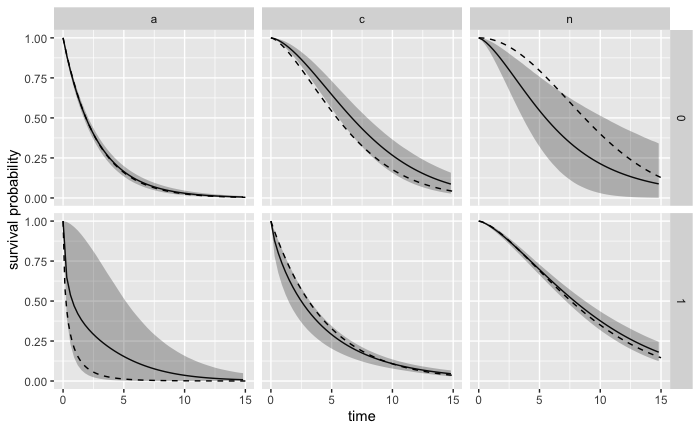
The estimated probabilities for three strata are respectively 0.234 (CI: 0.222 to 0.245), 0.611 (CI: 0.596 to 0.627) and 0.155 (CI: 0.145 to 0.165), close to the true values 0.25, 0.60 and 0.15. With \codeplot(), we can view the estimated survival probability curves and their $95\%$ confidence regions visually (Figure 4. The true survival probability curves are added for reference.

Refer to caption — Figure 4: Plot of estimated survival probability curves (solid) with 95% confidence region (shaded). The true survival probability curves are also plotted (dashed).

5.4 Case 4: Data with cluster effects

We simulate a randomized experiment with $N=1,000$ units. We assign $S\in\{(0,0),(0,1),(1,1)\}$ independently with probability 0.25, 0.50 and 0.25, respectively. The treatment assignment $Z_{i}$ is independently drawn from a $Bernoulli(0.5)$ . To mimic the existence of clusters, we randomly assign these units to 10 clusters, denoted by $C_{i}=j$ . We sample random effect $\xi_{j}$ from the standard normal distribution for each cluster $j$ . Conditional on the stratum $S$ and treatment assignment $Z$ , the outcome $Y$ follows a gaussian distribution where

	$\displaystyle Y\mid S=(0,0),Z=z,X_{1},X_{2},C=j$	$\displaystyle\sim\mathcal{N}(X_{1}-X_{2}+\xi_{j},0.3)$
	$\displaystyle Y\mid S=(0,1),Z=z,X_{1},X_{2},C=j$	$\displaystyle\sim\mathcal{N}(2X_{1}-(1+z)X_{2}+2+6z+\xi_{j},0.2)$
	$\displaystyle Y\mid S=(1,1),Z=z,X_{1},X_{2},C=j$	$\displaystyle\sim\mathcal{N}(X_{1}+X_{2}-1+\xi_{j},0.2).$

{CodeChunk}{CodeInput}

R> fit <- PStrata( + S.formula = Z + D 1, + Y.formula = Y X1 + X2 + (1 | C), + Y.family = gaussian(), + data = data, + strata = c(n = "00*", c = "01", a = "11*"), + prior_intercept = prior_normal(0, 1), + warmup = 1000, iter = 2000, + cores = 6, chains = 6, refresh = 10 + ) R> summary(fit) {CodeOutput} mean sd 2.5n 0.2806836 0.01412599 0.2520836 0.2711908 0.2800077 0.2902168 0.3083786 c 0.5202746 0.01656015 0.4871375 0.5084747 0.5208637 0.5312158 0.5520182 a 0.1990418 0.01242839 0.1757518 0.1901582 0.1988140 0.2076523 0.2224745 {CodeInput} R> outcome <- PSOutcome(fit) R> contrast <- PSContrast(outcome, Z = TRUE) R> summary(contrast, "matrix") {CodeOutput} mean sd 2.5n:1-0 0.000000 0.0000000 0.000000 0.000000 0.00000 0.000000 0.000000 c:1-0 5.977509 0.0178666 5.943497 5.965294 5.97707 5.989835 6.012452 a:1-0 0.000000 0.0000000 0.000000 0.000000 0.00000 0.000000 0.000000

	True value	Posterior mean	$2.5\%$ quantile	$97.5\%$ quantile
$\mathrm{Pr}(S=(0,0))$	0.300	0.281	0.252	0.308
$\mathrm{Pr}(S=(0,1))$	0.500	0.520	0.487	0.552
$\mathrm{Pr}(S=(1,1))$	0.200	0.199	0.176	0.222
$\E[Y(1)-Y(0)\mid S=(0,1)]$	6.000	5.978	5.943	6.012

Table 7: The posterior summary of important quantities with true values in Simulation 4.

6 Summary

Principal Stratification is an important tool for causal inference with post-treatment confounding. This paper introduces the \pkgPStrata package and demonstrates its use in the most common settings of non-compliance with single and two post-treatment variables. \pkgPStrata is under continuing development; future versions will include the settings of truncation by death and informative missing data, as well as graphic diagnostics.

Computational details

\pkg

PStrata 0.0.1 was built on \proglangR 4.0.3 and dependent on the \pkgRcpp 1.0.6 package, the \pkgdplyr 1.0.7 package, the \pkgpurrr 0.3.4 package, the \pkgrstan 2.21.1 package, the \pkglme4 1.1-27.1 package, the \pkgggplot2 3.3.6 package and the \pkgpatchwork 1.1.1 package. All these packages used are available from the Comprehensive \proglangR Archive Network (CRAN) at https://CRAN.R-project.org/.

Acknowledgement

This research is supported by the Patient-Centered Outcomes Research Institute (PCORI) contract ME-2019C1-16146. We thank Laine Thomas and Peng Ding for helpful comments.

References

Abrams et al. (1996) Abrams K, Ashby D, Errington D (1996). “A Bayesian approach to Weibull survival models—Application to a cancer clinical trial.” Lifetime Data Analysis, 2(2), 159–174.
Angrist et al. (1996) Angrist J, Imbens G, Rubin D (1996). “Identification of causal effects using instrumental variables.” Journal of the American Statistical Association, 91(434), 444–455.
Cox (1972) Cox DR (1972). “Regression Models and Life-Tables.” Journal of the Royal Statistical Society: Series B (Methodological), 34(2), 187–202.
Frangakis and Rubin (2002) Frangakis C, Rubin D (2002). “Principal Stratification in Causal Inference.” Biometrics, 58(1), 21–29.
Gilbert and Hudgens (2008) Gilbert P, Hudgens M (2008). “Evaluating candidate principal surrogate endpoints.” Biometrics, 64(4), 1146–1154.
Hirano et al. (2000) Hirano K, Imbens G, Rubin D, Zhou XH (2000). “Assessing the effect of an influenza vaccine in an encouragement design.” Biostatistics, 1, 69–88.
Imbens and Rubin (1997) Imbens G, Rubin D (1997). “Bayesian inference for causal effects in randomized experiments with noncompliance.” The Annals of Statistics, 25(1), 305–327.
Jiang et al. (2016) Jiang Z, Ding P, Geng Z (2016). “Principal causal effect identification and surrogate end point evaluation by multiple trials.” Journal of the Royal Statistical Society: Series B (Statistical Methodology), 78(4), 829–848.
Jiang et al. (2022) Jiang Z, Yang S, Ding P (2022). “Multiply robust estimation of causal effects under principal ignorability.” JRSSB.
Jo and Stuart (2009) Jo B, Stuart E (2009). “On the use of propensity scores in principal causal effect estimation.” Statistics in Medicine, 28(23), 2857–2875.
Mcdonald et al. (1992) Mcdonald C, Hui S, Tierney W (1992). “Effects of Computer Reminders of Influenza Vaccination on Morbidity during Influenza Epidemics.” M.D. computing : computers in medical practice, 9, 304–12.
Rubin (2006) Rubin D (2006). “Causal inference through potential outcomes and principal stratification: application to studies with censoring due to death.” Statistical Science, 91, 299–321.
Wei (1992) Wei LJ (1992). “The accelerated failure time model: A useful alternative to the cox regression model in survival analysis.” Statistics in Medicine, 11(14-15), 1871–1879.
Zhang et al. (2009) Zhang J, Rubin D, Mealli F (2009). “Likelihood-based analysis of the causal effects of job-training programs using principal stratification.” Journal of the American Statistical Association, 104, 166–176.