2023
Real-world datasets are often of high dimension and effected by the curse of dimensionality. This hinders their comprehensibility and interpretability. To reduce the complexity feature selection aims to identify features that are crucial to learn from said data. While measures of relevance and pairwise similarities are commonly used, the curse of dimensionality is rarely incorporated into the process of selecting features. Here we step in with a novel method that identifies the features that allow to discriminate data subsets of different sizes. By adapting recent work on computing intrinsic dimensionalities, our method is able to select the features that can discriminate data and thus weaken the curse of dimensionality. Our experiments show that our method is competitive and commonly outperforms established feature selection methods. Furthermore, we propose an approximation that allows our method to scale to datasets consisting of millions of data points. Our findings suggest that features that discriminate data and are connected to a low intrinsic dimensionality are meaningful for learning procedures.
Selecting Features by their Resilience to the Curse of Dimensionality
keywords
Feature Selection, Curse of Dimensionality, Intrinsic Dimension1 Introduction
Contemporary datasets are of high dimension and their complexity continues to increase. Thus, information derived by machine learning procedures is rarely comprehensible or interpretable. This includes even procedures originally categorized as explainable, such as decision trees. Addressing this problem, a variety of works aims to simplify data through methods that reduce size or, in particular, the dimensionality. An important class of such methods has the emblematic name feature selection (FS). By simply selecting to be discarded feature dimensions, they preserve the explainability of the remaining original dimensions, in contrast to approaches such as principal component analysis. Although there are supervised and unsupervised types of FS, only unsupervised procedures are suited to improve the understanding of data regardless of a specific learning task. Moreover, they do not require costly label information.
One important phenomenon which underlies the complexity of high dimensional data is the curse of dimensionality. The curse of dimensionality is a broad term which is used for different phenomenons that arise in the context of high-dimensional data. In this work, we follow the definition of Pestov 2007. According to Pestov, the curse of dimensionality describes the situation where features are concentrated to specific regions and therefore do not allow to discriminate different data points. Data that is strongly affected by this phenomenon is considered to be of high intrinsic dimension (ID). Yet, in common feature selection methods, the curse of dimensionality is rarely explicitly accounted for, even though it does a) demonstrably influences learning success in high-dimensional real-world scenarios, and b) potentially prevent common FS methods to choose the best features to learn from. Thus, it is crucial to incorporate the intrinsic dimension into the process of feature selection.
We meet this challenge by proposing an unsupervised feature selection method that picks features based on their measurable ability to discriminate different data points. While other methods are based on feature relevance measures, such as variances, or select features by discarding strongly correlated ones, our method ranks features by their resilience against the curse of dimensionality in the sense of Pestov. For this, we build on recent work (Hanika et al 2022; Stubbemann et al 2023) which studies intrinsic dimensionality for geometric datasets. By adapting corresponding ideas for computing the intrinsic dimensionality, we derive an algorithm that allows to find precisely those features that are able to tame the influence of the curse of dimensionality. Furthermore, adapting the speed-up techniques proposed in Stubbemann et al 2023 will allow feature selection in settings with large-scale datasets comprised of millions of data points. While (Hanika et al 2022) and (Stubbemann et al 2023) are focused on computing the intrinsic dimensionality of datasets, we will rank and select individual features by their ability to discriminate data points. Thus, we identify features that are harmed by the curse of dimensionality by a comparable low extent.
We experimentally show on real-world datasets that features selected by our proposed method are meaningful to learn from. To be more specific, we experiment on the OpenML-CC18 Curated Classification benchmark (Open18) (Bischl et al 2019) and witness that our method is competitive or even outperforms established feature selection methods with respect to feature selection for classification tasks. Furthermore, we use the Open Graph Benchmark (Hu et al 2020) to show that our method is capable of feature selection for large-scale learning with Graph Neural Networks. To sum up, our experiments indicate that features that are able to discriminate data and thus weaken the curse of dimensionality are highly relevant for learning tasks. Our code is publicly available.11 1 https://github.com/mstubbemann/FSCOD
2 Related Work
We focus on unsupervised feature selection, which is an established research topic (Solorio-Fernández et al 2020; Cai et al 2018; Alelyani et al 2018). Established methods are often focused on the identification of outstanding features by identifying the relevant features for clustering (Dy and Brodley 2004; Breaban and Luchian 2011; Dutta et al 2014). Another directions focuses on selecting a subset of important and dissimilar features (Zhao and Liu 2007; Ferreira and Figueiredo 2012; Mitra et al 2002; Hanika et al 2019). Here, feature importance can for example be measured via variances and similarities via correlation coefficients. While applying such methods may result in a decreasing intrinsic dimensionality, they do not explicitly account for the curse of dimensionality in the selection process.
A small amount of research has incorporated intrinsic dimension estimators into feature selection (Gómez et al 2010; Golay and Kanevski 2017; Mo and Huang 2012; Faloutsos et al 2010). However, these method either only use the ID to determine the amount of features to select (Gómez et al 2010) or they are based on recomputing intrinsic dimensionalities after discarding features which limits scalability (Golay and Kanevski 2017; Mo and Huang 2012). Even if applicable to larger datasets, these methods build on notions of intrinsic dimensionality that do not aim to quantify the curse of dimensionality (Faloutsos et al 2010). Instead, these notions work under the assumption that the data lies on a manifold of lower Euclidean dimension. The goal of the ID notion is then to approximate the dimension of this manifold.
In contrast, we build our feature selection procedure on a notion of ID which quantifies the influence of the curse of dimensionality which occurs when data points can not be discriminated. In the works of Pestov (Pestov 2000; Pestov 2007; Pestov 2008), all Lipschitz functions are considered as potential features to discriminate data, which often hinders the practical computation. This was tackled by defining intrinsic dimensionality for geometric datasets (Hanika et al 2022), where a set of features to consider can be defined beforehand. The computation and approximation on large-scale real world data has recently been made possible (Stubbemann et al 2023). We use these findings to incorporate Pestovs notions of the curse of dimensionality in the process of unsupervised feature selection. Note, that Hanika et al 2022 and Stubbemann et al 2023 were solely focused on the intrinsic dimensionality of datasets and thus of the question how all features together can discriminate data points. In contrast, we present a novel approach to rank and select individual features by their ability to discriminate data points.
3 Feature Selection via Discriminability
We present our work in a general setting for datasets, i.e., for geometric datasets (Hanika et al 2022), where is a set of data points and is a set of feature functions from to . We require , where . Furthermore, has to be a complete and separable metric space with being a Borel probability measure on .
From this point on, we consider the special case of finite geometric datasets, i.e., , with being the normalized counting measure. Hanika et al 2022 derived an axiomatization for functions to be dimension functions of geometric datasets. This axiomatization is based on the concentration of measure phenomenon (Gromov and Milman 1983; Milman 1988; Milman 2000) and its linkage to the curse of dimensionality by Pestov (Pestov 2000; Pestov 2007; Pestov 2008; Pestov 2010). The latter defines the curse of dimensionality as the phenomenon of features concentrating near their means or medians and not being able to discriminate data. To quantify this phenomenon the partial diameter is used, which determines to which extent a feature can discriminate sets of a specific measure . For finite geometric datasets the partial diameter has the form
where . Based on this, the observable diameter reflects how the feature set can discriminate data of a specific measure. More formally, . This notions allows to determine for a geometric dataset the ability of to discriminate the data points in . This is done by considering the Observable Diameter over all possible values for via
which has in the case of finite geometric datasets the form
| (1) |
as shown in Stubbemann et al 2023. With the usage of the notation , and the discriminability can be rewritten as
| (2) |
In the following, we consider feature selection with a fixed feature budget in an unsupervised setting, i.e., without any known labels of a specific classification task at selecting time.
Problem Statement.
Given a finite geometric dataset and a natural number , select the most important features of .
3.1 Selection of Discriminating Features
The definition of discriminability as in Equation 1 and Equation 2 quantifies to which extent the set of all features can discriminate data subsets of different cardinality. The main idea of our feature selection algorithm is to rank features by their ability to discriminate data subsets of different cardinality by solely using this feature.
Definition 1 (Discriminability).
The discriminability of with respect to feature is defined as
| (3) |
Enhancing Robustness against Outliers
Note, that one data point with an outstanding value can have a strong influence on via drastically increasing . To weaken this phenomenon, we propose to weight higher for smaller values of . This leads to the following definition.
Definition 2 (Normalized Discriminability and Normalized Intrinsic Dimensionality).
The normalized discriminability of with respect to which we define as
| (4) |
The normalized intrinsic dimensionality of with respect to is then given via
| (5) |
We then can rank features by their discriminability and select the features with the highest discriminability/ lowest intrinsic dimensionality. We call the resulting method features selection via discriminability (FSD). It is depicted in Algorithm 1.
3.2 Discarding Highly Correlated Features
Our methods select features by their ability to separate data points. However, it does not consider connections between individual features, as for example correlations. Thus, if for example the two features that separate the data set are nearly identical our method may select both as though selecting one of these features would be sufficient as the second one gives no extra information. To prevent such cases, we propose to incorporate correlation coefficients into our feature selection process, if desired. In order to do so, we define an additional number of features to remove via correlation coefficients. We then iteratively discard one of the two features with the maximal pearson correlation coefficient. The version of our algorithm that incorporates this preprocessing is called Feature Selection via Discriminability and Correlation (FSDC).
4 Feature Selection for Large-Scale Data
Since computing is in for fixed (Stubbemann et al 2023), computing is in . Hence, we have a worst case runtime which scales quadratic with . Thus, FSD(C) is applicable to medium-sized data sets with thousands of data points. However, it is not tailored to large-scale data with millions of data points.
Earlier work (Stubbemann et al 2023) has used so called support sequences, i.e. strictly increasing finite sequences of the form to approximate and by only computing for .
Inspired by this, we approximate the discriminability and intrinsic dimensionality with respect to a feature . The approximation is based on the result, that the map is monotonically increasing (Stubbemann et al 2023). Using this result, we replace for the value by or . More formally, we get the following definition.
Definition 3 (Upper and Lower Normalized Discriminability).
For a feature and a support sequence we call
the upper normalized discriminability with respect to and and
he lower normalized discriminability with respect to and .
Definition 4 (Upper, Lower and Approximated Normalized Intrinsic Dimensionality).
We define the upper/lower normalized intrinsic dimensionality with respect to and via and . We then rank the features in descending order by their approximated normalized intrinsic dimensionality with respect to and which is defined via
| (6) |
The resulting algorithm for large-scale datasets is depicted in Algorithm 2. We rank features via ascending . If we want to select features, we choose the first features of the resulting order.
4.1 Error Ratios of Approximations
Note, that as defined in Equation 6 only gives an approximation of as defined in Equation 5. Thus ranking the features by instead of may lead to a different ordering. We are interested in the amount of such changes. Let be the list of the features in ordered by ascending .
Definition 5 (Error Ratio).
The error ratio of is then given by
| (7) |
Computing for all is especially of interest when computing is not feasible. In such circumstances, it is also not possible to compute . Hence, we need an approximation or upper bound of which can be computed without needing .
Definition 6 (Maximal Error Ratio).
We define the maximal error ratio of via
| (8) |
The maximal error ratio can be computed without knowing for all . Per definition it holds that . Thus, for given features with we can conclude . Thus, we get the following corollary.
Corollary 1.
For each support sequence it holds that
| (9) |
To sum up, we now have an approximation algorithm which allow us to rank the features by their intrinsic dimensionality and we can efficiently bound the amount of errors this approximation produces. We denominate this method with large-scale feature selection via discriminability (and correlation)(LSFSD(C)).
5 Experiments
In the following we empirically examine the following hypothesis. Discriminative features are meaningful features with respect to learning performances. The aim is not to develop a new feature selection procedure that surpasses all established methods. Thus, we do not compare with all state-of unsupervised feature selection procedures. Instead we use a small set of representative baselines that consists of established methods and common-sense baselines based on correlation and variances. Furthermore, we compare our approach to random feature selection to evaluate if our features are indeed meaningful with respect to classification.
In all our experiments, we consider the features to be the coordinate projections, i.e., the feature functions are given via the data columns. We evaluate our feature selection method regarding to classification performances. We experiment with a Logistic Regression classifier on the OpenML-CC18 Curated Classification benchmark (Open18)22 2 https://www.openml.org/search?type=study&study_type=task&id=99&sort=tasks_included (Bischl et al 2019). To further evaluate our selection procedure on modern large-scale data we also select features for classification with Graph Neural Networks (GNNs) on a subset of the Open Graph Benchmark (Hu et al 2020). In both experiments, we evaluate how to classify on a small subset of the features. To be more detailed, we only want to keep 10% of all features. We evaluate our feature selection with and without the preprocessing procedure of Section 3.2. In the case with the preprocessing step, we use it do discard 10% of the features. In both experiments, we will also report results for classification on the full feature set. We evaluate against the following baselines.
- •
Random. Randomly selecting the 10% of features.
- •
Correlation Based. Only use the correlation based feature selection as proposed in Section 3.2 until only 10% of the features are left.
- •
Variance Based. Select the 10% of the features with the highest variance. We choose this baseline because it is a straight forward approach to for selecting features by their individual importance.
- •
SPEC.(Zhao and Liu 2007) SPEC first builds a complete graph between the individual data points with edge weights indicating similarities of the points and then uses spectral graph theory for estimating feature relevance. In our experiments, we use an RBF Kernel for similarity and evaluate feature relevance via . For details, we refer to Zhao and Liu 2007. We choose this baseline because it was the univariate filter method with the highest classification accuracy in a recent survey on unsupervised feature selection (Solorio-Fernández et al 2020).
- •
RRFS.(Ferreira and Figueiredo 2012) RRFS combines a function @sim which measures similarity of feature pairs and a relevance measure @rel that evaluates the importance of features. It iteratively chooses the next most relevant feature that has a similarity to the last chosen feature which below a specific threshold . For comparison, we choose to be the correlation coefficient value of the last pair of features that was used to discard a feature via Section 3.2. We use the Pearson correlation coefficient for similarity evaluation and evaluate the relevance of features via their variance. For more details, we refer to Ferreira and Figueiredo 2012. We use this baseline because it was the multivariate filter method with the highest classification accuracy in the survey mentioned above (Solorio-Fernández et al 2020).
5.1 Feature Selection for Logistic Regression
| Task ID | Dataset | Full | FSDC | FSD | Random | Corr | Vari | RRFS | SPEC | |
|---|---|---|---|---|---|---|---|---|---|---|
| 14 | mfeat-fourier | 76 | .813 | .694 | .753 | .433.032 | .457 | .751 | .751 | .630 |
| 16 | mfeat-karh. | 64 | .958 | .695 | .822 | .466.028 | .288 | .810 | .810 | .680 |
| 45 | splice | 60 | .918 | .531 | .611 | .580.026 | .534 | .725 | .647 | .806 |
| 9910 | Bioresponse | 1776 | .754 | .745 | .751 | .704.008 | .739 | .747 | .707 | .550 |
| 9977 | nomao | 118 | .947 | .907 | .907 | .835.012 | .752 | .793 | .793 | .759 |
| 9981 | cnae-9 | 856 | .944 | .884 | .884 | .391.032 | .404 | .888 | .144 | .128 |
| 9985 | 1st-order | 51 | .479 | .434 | .434 | .420.002 | .416 | .419 | .419 | .418 |
| 167125 | Internet-Advertisment | 1558 | .971 | .962 | .963 | .936.003 | .899 | .963 | .963 | .877 |
We select features as explained above and then use a Logistic Regression classifier. We use the data splits that are provided by Open18 and report mean test accuracies over all splits. We report means over 10 runs of this experiment. Note, that the Logistic Regression of Scikit Learn (Pedregosa et al 2011) using the default solver leads to deterministic results. As only the random selection method is non-deterministic, this is the only baseline where results of different repetitions vary.
We only experiment on a subset of Open18. To be more detailed, we discard all datasets with NaN values or only binary features. Furthermore, we discard all datasets where the Logistic Regression classifier of Scikit-Learn was not always able to converge on the full feature set. We use default parameters with the exception that we changed the maximal iterations from to to increase the chance of convergence. Finally, we arrive at out of datasets of Open18. The results are depicted in Table 1.
5.1.1 Results and Discussion.
For all datasets, FSD outcompetes the random baseline and for 7 out of 8 datasets FSDC outperforms random selection. Hence, selecting features by their discriminability a reasonable aproach to identify relevant features for learning. Furthermore, for out of baselines, FSD surpasses all baselines. This indicates that our selection approach is competetive with established feature selection methods.
Adding the correlation-based feature selection to FSD does not increase performances and feature selection solely based on correlation coefficients leads to comparable low accuracies. Furthermore, RRFS, which, in our configuration, combines feature variances with dropping strongly correlated features does not surpass the selection of features solely based on variance. All this indicates that the incorporation of correlation between features is not useful in this scenario. It also stands out, that FSDC sometimes lead to the same accuracy than FSD. In these cases it stands to reason that FSD does not select any features that are dropped by FSDC as preprocessing.
Overall, selecting only 10% often lead to a high drop compared to the original accuracy, indicating that such a small feature budget often not allows for sufficient feature selection. Thus, our experiment mainly gives insights in cases where feature selection is done because only using a small subset of features is computational feasible or to get new insights into the data and classification behavior. It is primarily not designed for feature selection to enhance classification accuracy. Here, the amount of selected features should be set higher. However, the competitiveness of our approach supports our hypothesis that discriminability of features is connected to their relevance for learning.
5.2 Feature Selection for Graph Neural Networks
| Dataset | Full | LSFSDC | LSFSD | Random | Corr | Vari | RRFS | |
|---|---|---|---|---|---|---|---|---|
| arxiv | 128 | |||||||
| products | 100 | |||||||
| mag | 128 |
We now evaluate to which extent our feature selection methods helps to select features for training Graph Neural Networks. For this, we use ogbn-arxiv, ogbn-mag and ogbn-products33 3 https://ogb.stanford.edu/docs/nodeprop/ from Open Graph Benchmark (Hu et al 2020). These datasets are fundamentally larger then the ones from Open18, with a nodeset size of (ogbn-arxiv), (ogbn-products) and (ogbn-mag).
To use LSFD(C) we need to choose a support sequence. As in Stubbemann et al 2023, we use log scale spacing. For this, we first choose a geometric sequence of length with and and use the support sequence which results from via discarding duplicated elements.
For training and classification, we use a plain SIGN model (Rossi et al 2020) with one hidden-layer of dimension and do hop neighborhood aggregation. We train with an Adam optimizer with learning rate of and weight decay of . We train for a maximum of epochs with a patience of epochs with respect to validation accuracy. We use a batch size of . We dropout at the input layer with a probability of and at the hidden layer with probability of for ogbn-arxiv, ogbn-products and ogbn-mag, respectively.
We report test accuracies, displaying means and standard deviations over rounds. We use all methods and baselines reported above. For SPEC, computation of the RBF kernel was not possible on our Server with GB RAM due to memory costs. This was true for using Scikit-Learn as well with plain numpy. The results are depicted in Table 2.
5.2.1 Results and Discussion.
In this experiment, preprocessing via Section 3.2 indeed can help as LSFSDC lead to higher accuracies then using LSFSD for ogbn-mag. LSFSDC also surpasses feature selection based solely on correlations. Note, that RRFS, the other method that combines similarities between features and selection by some measure of feature relevance, do lead to fundamentally worse results. Thus, one can not follow that combining similarity and relevance is the general key to successful feature selection. This is supported by the fact, that feature selection solely based on feature variance leads to high accuracies. For ogbn-products and ogbn-arxiv, LFSD lead to the best performance, for ogbn-mag, the highest accuracy is reached with LSFSDC. In this experiment, our selection method is again competitive with the baselines and surpasses random selection. This supports the hypothesis that selecting features via their discriminability is meaningful.
6 Parameter Study on Maximal Errors
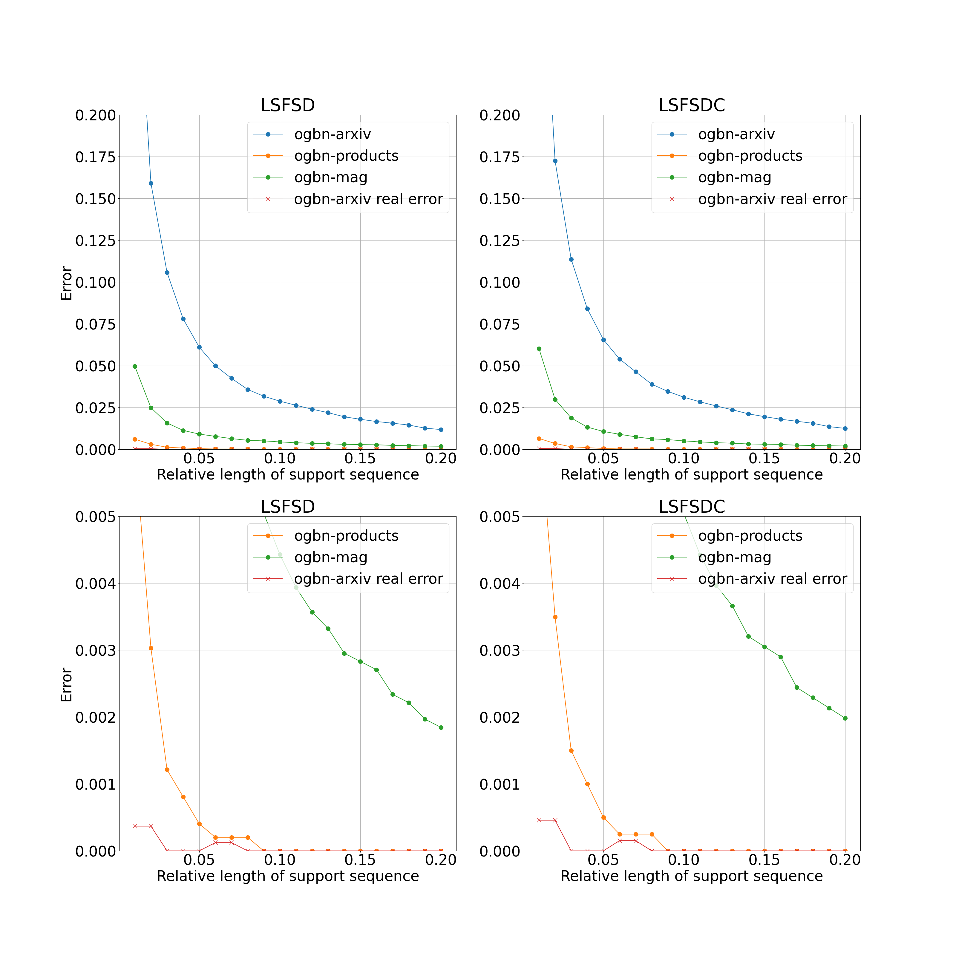
We now study the influence of the lengths of support sequences on the maximal error . For this, we generate the support sequence as in Section 5.2 with varying value . To be more detailed, we iterate through , where is the amount of points in the respective datasets. Here, if , we call the relative length of . Note, that the final support sequence may have a lower amount of elements in as we discard doubled elements. For all three ogbn datasets mentioned above, we display the maximal errors with the procedure mentioned in Section 3.2 and without. Since for ogbn-arxiv the exact computation of is possible, we also compute the “real” error for this dataset.
6.1 Results and Discussion
The results are depicted in Figure 1. We first note that the behavior of the maximal errors is not fundamentally effected by the decision for or against discarding strongly correlated features. In both settings, the curves behave similar. Only the absolute values tend to be lower when no discarding is done. Hence, the following observation and arguments hold for both cases.
For the larger datasets, ogbn-products and ogbn-mag, the maximal error is negligible for comparable small relative support sizes. For relative support sizes of , the maximal mistakes are under . For ogbn-arxiv we have an maximal error of around for this relative support size and overall higher maximal errors for all relative support lengths.
Comparing and for ogbn-arxiv it stands out, that the maximal error is a strong overestimation of the error . As computing for both other datasets is not feasible, we can not verify whether this is also the case for them. However, we know because of Equation 9, that is bound by the maximal error which is already negligible for ogbn-products and ogbn-mag.
7 Conclusion and Future Work
We proposed a novel unsupervised feature selection method that accounts for the intrinsic dimensionality of datasets. Our approach identifies those features that are able to discriminate data points and are thus responsible for taming the curse of dimensionality. Our experiments provide evidence that intrinsic dimension-based selection of features is competitive with well established procedures, occasionally outperforming them. Furthermore, we demonstrated that sampling techniques can be used to scale our feature selection method to more than millions of data points.
We identify as a natural next step for future work scenarios where the features are not given by coordinate projection, i.e., go beyond columns in tabular data. The generality of our modeling of features allows to encode, e.g., edge information for graphs. Thus, our method can be used for edge-sampling procedures that are important for training Graph Neural Networks. However, the question on how to encode graph information via feature functions is open.
While the present work emphasizes on understanding data by selecting features that break the curse of dimensionality, future work has to tackle as well the problem of understanding the behavior of specific model classes. This helps to further strengthen our understanding on the interplay between the success of learning and the presence of the curse of dimensionality.
Acknowledgement
The authors thank the State of Hesse, Germany for funding this work as part of the LOEWE Exploration project “Dimension Curse Detector" under grant LOEWE/5/A002/519/06.00.003(0007)/E19.
References
- Alelyani et al (2018) Alelyani S, Tang J, Liu H (2018) Feature selection for clustering: A review. Data Clustering pp 29–60
- Bischl et al (2019) Bischl B, Casalicchio G, Feurer M, et al (2019) Openml benchmarking suites. arXiv:170803731v2
- Breaban and Luchian (2011) Breaban M, Luchian H (2011) A unifying criterion for unsupervised clustering and feature selection. Pattern Recognition 44(4):854–865
- Cai et al (2018) Cai J, Luo J, Wang S, et al (2018) Feature selection in machine learning: A new perspective. Neurocomputing 300:70–79
- Dutta et al (2014) Dutta D, Dutta P, Sil J (2014) Simultaneous feature selection and clustering with mixed features by multi objective genetic algorithm. Int J Hybrid Intell Syst 11(1):41–54
- Dy and Brodley (2004) Dy JG, Brodley CE (2004) Feature selection for unsupervised learning. JMLR 5:845–889
- Faloutsos et al (2010) Faloutsos C, Wu L, Traina A, et al (2010) Fast feature selection using fractal dimension. Journal of Information and data Management 1(1):3–3
- Ferreira and Figueiredo (2012) Ferreira AJ, Figueiredo MAT (2012) An unsupervised approach to feature discretization and selection. Pattern Recognit 45(9):3048–3060
- Golay and Kanevski (2017) Golay J, Kanevski M (2017) Unsupervised feature selection based on the morisita estimator of intrinsic dimension. Knowledge-Based Systems 135:125–134
- Gromov and Milman (1983) Gromov M, Milman VD (1983) A topological application of the isoperimetric inequality. American Journal of Mathematics 105(4):843–854
- Gómez et al (2010) Gómez W, Leija L, Díaz-Pérez A (2010) Mutual information and intrinsic dimensionality for feature selection. In: 2010 7th International Conference on Electrical Engineering Computing Science and Automatic Control, pp 339–344
- Hanika et al (2019) Hanika T, Koyda M, Stumme G (2019) Relevant attributes in formal contexts. In: Int. Conf. on Conceptual Structures, Lecture Notes in Computer Science, vol 11530. Springer, pp 102–116
- Hanika et al (2022) Hanika T, Schneider FM, Stumme G (2022) Intrinsic dimension of geometric data sets. Tohoku Mathematical Journal 74(1):23 – 52
- Hu et al (2020) Hu W, Fey M, Zitnik M, et al (2020) Open graph benchmark: Datasets for machine learning on graphs. arXiv preprint arXiv:200500687
- Milman (1988) Milman V (1988) The heritage of p. lévy in geometrical functional analysis. Astérisque 157(158):273–301
- Milman (2000) Milman V (2000) Topics in asymptotic geometric analysis. In: Visions in Mathematics. Springer, p 792–815
- Mitra et al (2002) Mitra P, Murthy CA, Pal SK (2002) Unsupervised feature selection using feature similarity. IEEE Trans Pattern Anal Mach Intell 24(3):301–312
- Mo and Huang (2012) Mo D, Huang SH (2012) Fractal-based intrinsic dimension estimation and its application in dimensionality reduction. IEEE Trans on Knowl and Data Eng 24(1):59–71
- Pedregosa et al (2011) Pedregosa F, Varoquaux G, Gramfort A, et al (2011) Scikit-learn: Machine learning in Python. JMLR 12:2825–2830
- Pestov (2000) Pestov V (2000) On the geometry of similarity search: Dimensionality curse and concentration of measure. Inf Process Lett 73(1-2):47–51
- Pestov (2007) Pestov V (2007) Intrinsic dimension of a dataset: what properties does one expect? In: IJCNN 2007. IEEE, pp 2959–2964
- Pestov (2008) Pestov V (2008) An axiomatic approach to intrinsic dimension of a dataset. Neural Networks 21(2-3):204–213
- Pestov (2010) Pestov V (2010) Intrinsic dimensionality. ACM SIGSPATIAL Special 2(2):8–11
- Rossi et al (2020) Rossi E, Frasca F, Chamberlain B, et al (2020) SIGN: scalable inception graph neural networks. CoRR abs/2004.11198
- Solorio-Fernández et al (2020) Solorio-Fernández S, Carrasco-Ochoa JA, Martínez-Trinidad JF (2020) A review of unsupervised feature selection methods. Artif Intell Rev 53(2):907–948
- Stubbemann et al (2023) Stubbemann M, Hanika T, Schneider FM (2023) Intrinsic dimension for large-scale geometric learning. Transactions on Machine Learning Research URL https://openreview.net/forum?id=85BfDdYMBY
- Zhao and Liu (2007) Zhao Z, Liu H (2007) Spectral feature selection for supervised and unsupervised learning. In: Ghahramani Z (ed) ICML 2007, ACM International Conference Proceeding Series, vol 227. ACM, pp 1151–1157