Analyzing quantum entanglement with the Schmidt decomposition in operator space
Abstract
Characterizing entanglement is central for quantum information science. Special observables which indicate entanglement, so-called entanglement witnesses, are a widely used tool for this task. The construction of these witnesses typically relies on the observation that quantum states with a high fidelity to some entangled target state are entangled, too. We introduce a general method to construct entanglement witnesses based on the Schmidt decomposition of observables. The method works for two- and multi-particle systems and is strictly stronger than fidelity-based constructions. The resulting witnesses can also be used to quantify entanglement and to characterize its dimensionality. Finally, we present experimentally relevant examples, where our approach improves entanglement detection significantly.
Introduction.— In recent years, several experimental breakthroughs on different quantum technologies have been achieved. Examples are the demonstration of quantum supremacy with superconducting qubits arute, the implementation of quantum cryptography using a satellite Pan or in a device-independent manner nadlinger22; zhang22, and the study of quantum phases using digital quantum simulation Lukin. In such experiments large data sets are collected and the problem arises how to analyze them and connect them with the underlying quantum phenomena. For instance, if one wishes to reconstruct the density matrix of the quantum state arising in an experiment, methods like compressed sensing gross10, matrix-product-state tomography cramer10, shadow tomography huang20; nguyen22, and forms of overlapping tomography cotler20; yu23 have been designed.
For analyzing quantum correlations in experiments one frequently considers specific inequalities signaling the presence of correlations. The paradigmatic examples are Bell inequalities, whose violation signals the presence of quantum nonlocality brunnerbell. Bell inequalities do not rely on assumptions on the measurement devices, and if knowledge about at least some of the implemented measurements is given, steering inequalities uolasteering or entanglement witnesses rev4; rev5; rev6 are more efficient. In short, an entanglement witness is an observable with a nonnegative expectation value on all separable states, hence a negative expectation value signals the presence of entanglement. Clearly, finding all entanglement witnesses is a hard task, as it is equivalent to characterizing all entangled states, which is known to be an NP-hard problem gharibian10. Still, many constructions exist, often based on the idea of measuring the fidelity of the experimental state with some target state. If this fidelity is high enough, entanglement must be present.
In this paper, we present a method to analyze quantum entanglement based on the so-called Schmidt decomposition of operators. The Schmidt decomposition is a ubiquitous tool when analyzing pure two-particle quantum states, but it can also be applied to bipartite observables. Our method leads to novel entanglement witnesses, which outperform fidelity-based witnesses and tolerate significantly more noise when analyzing multiparticle entanglement. Our approach is computationally simple and can also be used to quantify entanglement or its dimensionality.
Entanglement and witnesses.— To start, recall that a bipartite quantum state shared by two parties, traditionally named Alice and Bob rev4; qibook is separable if it can be written as , where the form a probability distribution. If a state can not be written in this way, it is entangled, which is, for many quantum tasks, a necessary condition to outperform classical protocols curty04; pezze09. Unless stated otherwise, we assume that the dimensions of Alice’s and Bob’s space are the same,
For characterizing quantum entanglement, in experiments as well as in theory, entanglement witnesses have turned out to be useful rev6; bourennane; gezaspin, since they do not require full knowledge of the quantum state. As already mentioned, entanglement witnesses have a positive expectation value on separable states, so measuring a negative expectation value proves entanglement. For the construction of witnesses, several methods exist terhal; optimization; gezaspin; lurccnr; pianistates; dariusreview; HW; SIC, and one of the well-known key methods are witnesses based on the fidelity with a given pure target state. They are of the form where is some pure entangled target state. This witness expresses the fact that states with a high fidelity with , namely the ones with are entangled, too. Three remarks are in order. First, the coefficient can directly be computed. If is the Schmidt decomposition (with decreasingly ordered Schmidt coefficients and Schmidt rank ), it is given by the maximal squared Schmidt coefficient bourennane. Second, while fidelity-based witnesses are easy to construct, they have the disadvantage that they are not able to detect all entangled states, such as states with a positive partial transpose weilenmann20; faithful. Still, fidelity-based witnesses have the advantage that they can be extended easily to the multiparticle case by considering the Schmidt decompositions for the different bipartitions bourennane, this makes them the standard tool for analyzing entanglement in current experiments Nph1; Nph2; Nph3.
The main idea.— To introduce our main idea, let us start by pointing out the well-known fact that the Schmidt decomposition does not apply to pure states only, but also to observables. Indeed, one can decompose any operator acting on a bipartite space in the operator Schmidt decomposition (OSD) oS; oS2
| (1) |
Here, the are the operator Schmidt coefficients (OSC), chosen to be decreasingly ordered, and if is a quantum state, then the largest one encodes the maximal correlation between two appropriately normalized observables. Further, the (resp. ) form an orthonormal basis of Alice’s (Bob’s) operator space. This means that , examples of such bases are the appropriately normalized Pauli or Gell-Mann matrices. In fact, several works used the OSD, for example to analyze entanglement of mixed states cariello; cariello2; block; innsbruck or dynamics rescentOSD. We now write down our first main result, where we apply the OSD to a general operator :
Observation 1. Let be an operator with its OSD as in Eq. (1) and its largest OSC. Then
| (2) |
is an entanglement witness for bipartite entanglement.
Note that the choice of the parameter guarantees the positivity of the witness on separable states, but for general there may be proper witnesses with a smaller . This is in contrast to witnesses based on pure state fidelities, where is optimal. In order to prove the observation, it suffices to show that the expectation value is non-negative for an arbitrary pure product state ; this implies the statement for general separable states. First, writing in its OSD according to Eq. (1) it is clear that Then, for and and any orthonormal basis of the operator space one has , this follows from the fact that for the relation holds. So, by the Cauchy-Schwarz inequality we have and the Observation 1 follows.
From this simple construction of witnesses, several questions arise: How shall one choose the operator to detect a given entangled state ? Which states can be detected by this construction? What about the characterization of high-dimensional entanglement? Can this method be extended to the multiparticle scenario, in order to detect genuine multiparticle entanglement?
In the following, we will answer all these questions. For the moment, we would like to stress that the construction in Eq. (2) contains the pure state fidelity-based witness mentioned in the second paragraph as a special case, but still it is a more general description, so the OSD witnesses are strictly stronger. Indeed, starting from a pure state one can directly calculate the OSD of One finds nonzero operator Schmidt coefficients of the type , and the largest one is hence given by Thus, the pure state fidelity-based witness is indeed a special case of Eq. (2).
Schmidt number witnesses.— Let us now explain how the method of OSD witnesses can be used to characterize the dimensionality of entanglement, as characterized by the Schmidt number. Given the Schmidt decomposition of a pure state as above, the number of nonzero Schmidt coefficients is called Schmidt rank, and is known to be an entanglement monotone characterizing the dimensionality of entanglement Eisert. It can be generalized to mixed states as follows. If a mixed state cannot be written as a convex decomposition into pure states with Schmidt rank , then the mixed state has Schmidt number (SN) SN. Note that in this classification, mixed states with SN one are just the separable states, while entangled states have at least an SN of two.
Similar to entanglement witnesses, one can define Schmidt number witnesses as observables whose expectation values are positive for all states with SN such that a negative result indicates at least SN schmidtwit. In our scheme, these witnesses may be constructed analogously to Eq. (2), where the prefactor is replaced by a different number , which is a not necessarily optimal bound on the overlap of pure Schmidt-rank states with the operator . It turns out that these are simply given by the solution of a th order polynomial equation in the OSC of . For example, for SN we find . Then the witness detects only three-dimensional entanglement. However, for SNs greater than three, the prefactor is not so compact anymore, details on the computation of and the prefactors for higher SN are given in Appendix A. These witnesses can be seen as a generalization of the CCNR criterion for detecting Schmidt number (see also Observation 2 below), similar to the one in Ref. CCNRschmidt. But one can choose such that it certifies the SN of states, for which the CCNR extension CCNRschmidt fails, see also Appendix A.
Estimating bipartite entanglement monotones.— In many cases, one is not only interested in detecting quantum entanglement, but also wishes to quantify it and its resource character. For this quantification, many entanglement monotones have been proposed ppt; ppt1; negativity; negativity21; CREN; EOFde1; 2qubit1; 2qubit2; concurrence3; concurrence4; concurrence5; Gour; Fan; Uhlmann; GME1; GME2; GME21. A frequently used monotone is the concurrence EOFde1; 2qubit1; 2qubit2; concurrence3; concurrence4; concurrence5, defined for pure states as and for mixed states via the so-called convex roof construction (see Appendix B for details). This quantity is notoriously difficult to compute, but with the OSD witness, it can be directly estimated. Indeed, one can show that
| (3) |
where Note that Eq. (3) has a similar form of the result in Ref. chen, but interestingly analogous bounds can be derived for other measures, such as the convex-roof extended negativity CREN, the G-concurrence Gour; Fan; Uhlmann and the geometric measure of entanglement GME1; GME2; GME21, details are given in Appendix B. Moreover, they can finally be extended to the multiparticle case.
Optimization of OSD witnesses.— Having established basic properties of the OSD witness, we can now ask how to choose the observable in an optimal manner. Consider an entangled state that is detected by a witness as in Eq. (2) with the as in Eq. (1). Since we want to minimize the expectation value of the witness we can, without loss of generality, consider a witness where the the expectation values are positive for the given state and the are positive. In addition, the witness may be renormalized to achieve . But then it is clear that the optimal choice of the other is to take too.
So, an entangled quantum state is detected by a witness from Eq. (2) if and only if it can be detected by a witness of the form These witnesses, however, are characteristic for the computable cross norm or realignment (CCNR) criterion CCNR1; CCNR2; lurccnr and we have:
Observation 2. A bipartite quantum state can be detected by an OSD witness as in Eq. (2) if and only if it can be detected by the CCNR criterion.
The critical reader may ask at this point, why we have defined the OSD witnesses in the general form of Eq. (2) although the simpler subclass of CCNR witnesses contains all the relevant cases already. There are two reasons for that: First, as stressed above, the direct connection to the CCNR criterion does not hold for witnesses for a higher Schmidt number. Second, the form of the witness in Eq. (2) is the key for the generalization to multiparticle entanglement. There, we will search for multiparticle witnesses, which have the form as in Eq. (2) for any bipartition. Restricting then the attention to specific optimal witnesses for each bipartition does not lead to strong witnesses for the entire system Lancien and there is a trade-off between the optimality of the bipartite witness and the efficiency for multiparticle entanglement detection.
So, let us discuss how a given OSD witness can be gradually optimized, this will be central for the discussion of multiparticle entanglement later. We consider an entangled state (e.g., some pure state) which is affected by some separable noise (e.g., the maximally mixed state ). So, the total state is of the form and one can ask for the minimum of the required visibility , such that all states with are detected by the OSD witness.
A given OSD witness can be optimized in two directions. First, one may alter the coefficients in Eq. (1), second one may change the operators in the Schmidt decomposition. Let us first discuss the optimization of the OSC. For a given OSD witness, one can directly compute the and, leaving all other quantities fixed, this is a function of the parameters . Then, one can compute the gradient and minimize with some steepest descent algorithm (see Appendix C for details). We stress that after adjusting the in one iteration step one can calculate the updated in order to guarantee that the updated is indeed a proper witness, so no fake entanglement detection can arise from this procedure.
Second, we explain the optimization of the Schmidt operators while keeping the and fixed. Since the form an orthonormal basis, one can consider an infinitesimal rotation with being an infinitesimal rotation matrix of the form
| (4) |
with being the generator matrices of the . Finally, one can write as a function of the and optimize the via a gradient algorithm.
In practice, these two approaches work very well, even if the initial OSD witness was not chosen properly. For instance, for a bound entangled state (the so-called UPB state in -systems) the procedures directly find a witness that detects it, even if the initial witness was not capable of detecting it. Details on the optimization procedures and on the examples are given in Appendix C.
Multiparticle entanglement.— Now we are ready to present the extension of OSD witnesses to the multiparticle case. Let us first recall the notion of genuine multiparticle entanglement (GME) rev5. For the case of three particles, a pure state can be fully separable (e.g., ) or biseparable for some bipartition (e.g., , where is a two-qubit singlet state). Finally, a pure state is genuine multiparticle entangled if it is not biseparable with respect to any bipartition. Well-known examples of genuine multiparticle entangled states for three qubits are the Greenberger-Horne-Zeilinger (GHZ) state and the W state Similarly, one can define biseparability and genuine multiparticle entanglement of more than three particles.
The generalization to mixed states goes via convex combinations. A mixed state is fully separable, if it can be written as a convex combination of pure fully separable states, that is A state is biseparable if it can be expressed as a convex combination of pure biseparable states, these pure states may be biseparable with respect to different bipartitions. Finally, mixed states are genuine multiparticle entangled, if they are not biseparable.
For the characterization of genuine multiparticle entanglement, entanglement witnesses can be directly used again and a witness for GME is defined by the property that it is non-negative on all biseparable states. The method of OSD witnesses can directly be used to write down GME witnesses: Consider a tripartite operator . We can compute the OSD for the three bipartitions , and , resulting in three maximal Schmidt coefficients , , and Note that these are asymmetric scenarios for the OSDs, where the dimensions of the two sides are not the same. Then, taking as the maximum of these, the operator
| (5) |
has a positive expectation value on all pure biseparable states, hence it is a witness for genuine multiparticle entanglement; the generalization for more particles is described in Appendix E.
It is clear that the witness in Eq. (5) is more general than fidelity-based witnesses for multiparticle entanglement. Such fidelity-based witnesses have been a standard tool to analyze GME in experiments in the last years, so we will analyze in the following the advantage occurring from the construction in Eq. (5).
Examples of multiparticle states.— Now we are ready to use our methods to derive stronger witnesses for genuine multiparticle entanglement. In the following, we explain our approach for the three-qubit W state , the approach for other states is similar. A known witness for genuine multiparticle entanglement in the vicinity of the W state is acinprl2001
| (6) |
This can be viewed as an OSD witness from Eq. (5) with The recipe for its improvement is as follows. We consider as entangled target state and wish to maximize the robustness for the separable noise given by . For a given bipartition one can improve by adjusting the Schmidt coefficients or the Schmidt operators as outlined above. We then go through the bipartitions and for each bipartition we improve the witness by a combination of the two optimization methods. Numerical details of the procedure are given in Appendix C.
The starting witness in Eq. (6) requires a visibility of in order to detect GME. Already after some iterations of the optimization procedure one arrives at a witness for which the required visibility is reduced to , demonstrating the superiority of the OSD witness over the fidelity-based construction.
We have applied the same method to a variety of other multi-qubit states. This includes the three-qubit uniform hypergraph state 1404.6492 and the four-qubit W state , Dicke state and singlet-state rev5. For all these states we found a significantly improved noise robustness, see Table 1 for concrete values. Detailed forms of the states as well as the results for other states are given in Appendix C. Note that OSD witnesses do not improve the fidelity-based witness for the GHZ state, as this witness is known to be optimal for maximally mixed noise bounds15.
| state | visibility | visibility |
|---|---|---|
| 0.556 | ||
| 0.545 | ||
| 0.714 | ||
| 0.540 | ||
| 0.572 |
Analytical approaches.— Two analytical approaches are worth to be mentioned. First, it is also possible to construct the OSD witnesses analytically by starting from a pure high-dimensional quantum state and interpreting this as an operator on a lower-dimensional space. For instance, for the GHZ state on three four-level systems the vector Schmidt decomposition is directly given. Consequently, taking for arbitrary orthonormal bases , on three qubits will always result in an entanglement witness This ansatz can be generalized using arbitrary highly entangled pure states. Most importantly, given such a witness with a fixed structure, one can optimize the operators for given states by an iteration of purely analytical steps, which is indeed more general than a simple optimization over local unitary transformations. Details and examples are given in Appendix D. Second, note that the operators are actually local orthogonal observables. Thus we can use the results from Ref. chengjieCV to define the OSD witnesses for continuous variable systems, too.
Multipartite entanglement measures.— Again, the novel multiparticle witnesses can be made quantitative and be used to estimate monotones for genuine multiparticle entanglement. One possibility to build such monotones is to start with an entanglement monotone for pure two-particle states. Then, one can define for a multiparticle state the global entanglement as the minimum of for all bipartitions. Finally, one extends this to mixed states via the convex roof construction.
Such entanglement monotones can be directly estimated from the expectation value of the witness in Eq. (5). For instance, one may consider the multiparticle version of the concurrence. Then, one finds where and is, for the special case of tripartite systems the maximum of dimensions of Alice, Bob, and Charlie. This approach can be generalized to other measures and more particles, details are given in Appendix E.
Conclusion.— We have introduced a novel method to characterize entanglement for quantum systems of two or more particles. The resulting entanglement witnesses are strictly stronger than the widely used fidelity-based witness and can improve entanglement detection in realistic scenarios significantly. On the technical level, the approach does not involve advanced numerical tools such as semidefinite programming. The method can be seen as an extension of the CCNR criterion of separability to the multiparticle case, in the same sense as Ref. Jungnitsch presented an extension of the PPT criterion to the multiparticle case.
Several new lines of research emerge from our findings. First, it would be highly desirable to further characterize the resulting witnesses analytically for interesting families of quantum states. Second, entanglement witnesses can also be used to characterize other properties of quantum states, such as the teleportation fidelity teleportation, the distillability distillability, and the multipartite Schmidt vector Huber; SVec so it is relevant to apply our methods to these cases. Third, the statistical analysis of entanglement tests from finite data has become essential in the last years flammia, so our approaches also need to be analyzed from this viewpoint. Fourth, thinking of experimental implementations, it is desirable to give an estimation of the errors occurring when assuming small deviations of the desired measurements. In fact, for a special case of two-particle OSD witnesses this was recently discussed morelli, but it remains open to generalize this approach further and apply it to the multipartite case. Finally, in general, as fidelity-based entanglement witnesses have been used for many experiments, the presented improvement may allow for novel and exciting experiments.
We thank Jonathan Steinberg for discussions. This work is partially supported by the Innovation Program for Quantum Science and Technology (Grant No. 2021ZD0301200), the National Natural Science Foundation of China (Grant No. 11734015), and K. C. Wong Magna Fund in Ningbo University. S.D. and O.G. are supported by the Deutsche Forschungsgemeinschaft (DFG, German Research Foundation, project numbers 447948357 and 440958198), the Sino-German Center for Research Promotion (Project M-0294), the ERC (Consolidator Grant 683107/TempoQ), and the German Ministry of Education and Research (Project QuKuK, BMBF Grant No. 16KIS1618K). S.D. is further supported by the House of Young Talents of the University of Siegen. A.A. acknowledges the support from DAAD fund for bilateral project.
Appendix A Appendix A: Schmidt number witnesses
In this appendix, we discuss how OSD witnesses can be used to analyze the dimensionality of entanglement by characterizing the Schmidt number (SN) of quantum states. First, we explain in detail the derivation of witnesses for SN three, as mentioned in the main text. Then, we derive a construction for higher SNs. Finally, we present two examples which demonstrate the power of our methods. First, we present a quantum state whose SN can not be certified with fidelity-based witnesses, but with OSD witnesses. Second we present an example which shows that the OSD witnesses for SN are stronger than simple extensions of the CCNR criterion.
A.1 A1: Witnesses for SN three
We can use our scheme to construct SN witnesses according to . In order to compute the coefficient such that is indeed a SN witness one has to maximize the expression with respect to all pure states with Schmidt rank . This can be simplified by considering an upper bound: , where the and are the OSCs of and , respectively. Then, for the maximum of this expression can be found analytically, which results in maximizing a second order polynomial as mentioned in the main text; now we explain the details.
For the decreasingly ordered OSCs of the projector are given by the products of the vector Schmidt coefficients of the states , that is . The maximization then simplifies to
| (7) |
where the coefficients and obey the constraints , and . Taking a closer look at the function , one finds that it can also be written as a matrix vector multiplication
| (8) |
with the normalized vector and the matrix
Since the matrix is not necessarily symmetric, it needs to be symmetrized, such that Eq. (8) describes an eigenvalue problem, which is then solved by the largest eigenvalue of the matrix :
| (11) |
Then, the eigenvalues can be computed, which for the matrix are given by:
| (12) |
where we used the short-hand notations and . Since all as well as and are positive, the maximum eigenvalue is
| (13) |
Finally, we note that this value can indeed be reached with the given constraints on the . The coefficients of the eigenvector corresponding to the maximum eigenvalue of are all positive, since having a negative coefficient would make the expression smaller. Moreover, the eigenvector is normalized and therefore is fulfilled. The last condition the need to fulfill is that they should be ordered decreasingly ( ). This, however is guaranteed by the way the matrix and therefore is constructed. Since the OSCs are also in decreasing order and therefore , the first entry of the eigenvector maximizing Eq. (11) must be greater or equal to the second one, .
A.2 A2: Witnesses for higher SN
Now we consider witnesses certifiying SN . Therefore we want to find the coefficient such that the Schmidt witness has a non-negative expectation value on all states with SN . Proceeding analogously to the case , the OSCs of the projector are given by . To obtain the function , the OSCs have to be sorted decreasingly. In the case , however, there is no unique order: Depending on the actual values of the , one has either or . They also might be equal (), but then the order would not matter. This leads to two possible functions and that have to be considered:
| (14) |
The coefficient is then given by the maximum of those two functions:
| (15) |
This can be found by interpreting and in terms of matrices, analogously to the case . The corresponding matrices are given by
Proceeding as before, the coefficient is given by
| (22) |
where describes the maximum eigenvalue of and and are the symmetrized matrices and in Eq. (A.2). Since the are matrices, is the solution of a third order polynomial in the , which are the first nine OSCs of the operator . So, computing is numerically straightforward.
For SN higher than four, however, the computation is still straightforward but requires more effort. In these cases there are even more OSCs to arrange in decreasing order and therefore more possibilities to define the matrices occur. One can roughly estimate the number of matrices one has to check for a given SN using the concept of Young tableaux. A detailed discussion of this is given in Ref. ma.
A.3 A3: Two relevant examples
For our first example, we consider the mixed two-ququad state
| (23) |
with
| (24) |
which has SN three. Fidelity-based Schmidt witnesses here only detect Schmidt number two weilenmann20, which is equivalent to certifying entanglement. Using our scheme, however, we can construct a witness detecting the SN three of this state.
As already mentioned in the main text, for bipartite entanglement witnesses the best choice of the operator is taking the Schmidt operators from the target state and setting all OSCs to one. Thus it is a natural approach to choose the operator the same way for Schmidt witnesses. This yields and consequently, the Schmidt witness for SN three is given by
| (25) |
where the are the Schmidt operators of . This witness certifies SN three of the state with visibility .
We add that for the special choice of the coefficient reduces to . This is due to the fact that in this case there is only one possibility to arrange the OSCs in a matrix , namely a matrix with all entries equal to one. These matrices have only one nonzero eigenvalue which is given by . Note that this form of the witness corresponds to an extension of the CCNR criterion. Indeed, as shown in Ref. CCNRschmidt the CCNR criterion can also be applied to characterize the dimensionality of entanglement; one has if the state has SN .
Still, with our second example we show that the OSD witnesses for the SN also detect states where the extended CCNR criterion fails. To do so, consider the pure two-ququad state
| (26) |
where . This state has SN three and is detected by the fidelity-based witness faithful, which is a special case of the OSD Schmidt witness. However, computing the sum of the OSCs of one finds that and hence SN three is not certified by the extended CCNR criterion.
Note that there are further results on the Schmidt number detection which are at least as good as our first example Shuheng; Nikolai. However, from the experimental point of view they rely on different methods. So, giving the exact relation between those criteria and the OSC witnesses is left for future studies.
Appendix B Appendix B: Estimating bipartite entanglement monotones
In this section, we explain how some entanglement measures can be estimated from the OSD witness. First, we explain how the sum of the Schmidt coefficients of a pure state can be estimated from the expectation value of an OSD witness. Second, we prove that if some entanglement measure is a certain function of the sum of the Schmidt coefficients for pure states, then the value of the measure for mixed states can be estimated from the witness value. Finally, for several entanglement measures a suitable functional relation with the sum of the Schmidt coefficients is already known from the literature observe1, this then gives explicit bounds on the measures from the OSD witness. We start with the following Lemma.
Lemma 1. Consider a pure state in the Schmidt decomposition with being its Schmidt coefficients in decreasing order. Then one has
| (27) |
where is an arbitrary Hermitian operator as in Eq. (2) in the main text.
Proof. We start from the right-hand side of Eq. (27). Defining and one has
| (28) | |||||
where we have used the Cauchy-Schwarz inequality, , and and .
Then we can formulate the following theorem.
Theorem 2. Consider an entanglement measure for bipartite states defined via the convex roof construction and suppose that for pure states
| (29) |
with , and is the vector containing the Schmidt coefficients. Let us define the function as
| (30) |
and is the convex hull of (that is the largest convex function smaller or equal to ). If is a monotonously increasing function in , then for an arbitrary bipartite mixed state with dimension (), one has
| (31) |
Proof. Assume that is the optimal decomposition for to achieve the infimum of . Then we have
| (32) | |||||
where we have used , and
| (33) |
based on Lemma 1, and is a monotonously increasing convex function.
Finally, we can write down the lower bounds on entanglement measures:
Corollary 3. For many entanglement measures the corresponding functions are known observe1. Specifically, based on Theorem 2, one can obtain lower bounds on the convex-roof extended negativity (CREN) CREN, concurrence EOFde1; 2qubit1; 2qubit2; concurrence3; concurrence4; concurrence5, G-concurrence Gour; Fan; Uhlmann, and geometric measure of entanglement GME1; GME2; GME21 as follows,
| (34a) | |||||
| (34b) | |||||
| (34c) | |||||
| (34d) | |||||
where and is the smaller local dimension of the bipartite system. If we choose , the results of Eqs. (34a)-(34d) reduce to the results in Ref. observe1.
Appendix C Appendix C: Optimization of OSD witnesses
In this appendix we explain in detail how to optimize an OSD witness numerically. First, we will give an algorithm that optimizes the operator Schmidt coefficients (OSCs) of the operator . Then an algorithm which focuses on the optimization of the Schmidt operators will be introduced. Lastly, we will discuss the actual implementation for bipartite and multipartite systems
C.1 C1: Optimization with respect to the OSCs
First, recall that the OSD witness is given by , where is the largest OSC. In order to optimize the OSD witness for some target state , the goal is to minimize the required visibility , which is given by
| (35) |
for some noise . In the later examples, we typically choose to be the completely mixed state here. Using the definition of the OSD witness and writing in its OSD, we can express Eq. (35) as
| (36) |
and thus interpret it as a function of the . Here, it is important to mention, that A and B no longer refer to Alice and Bob as single parties, but considering a bipartition of the multipartite system, we denote the first subsystem as Alice’s part and the second one as Bob’s. Note that therefore, the OSD might be asymmetric which we will address in more detail in the next subsection. As we wish to minimize the visibility by updating the OSCs, we may apply a gradient descent algorithm. To do so, we start by computing the gradient of with respect to the OSCs yielding
| (37) |
for the -th entry of the gradient, where we used the short-hand notations and . Then, the witness can be improved applying the following algorithm.
Algorithm 1 (Optimization over Schmidt coefficients):
- •
Start with some input operator and compute the OSD witness.
- •
Write in the OSD.
- •
Compute the gradient of the required visibility using Eq. (37).
- •
Update the OSCs according to the update rule
(38) - •
Update the operator using the new OSCs:
(39) - •
Renormalize the updated operator by fixing the trace and compute the new maximum OSC .
Iterating those steps until the algorithm converges will improve the witness. The renormalization has the advantage that the expectation values of the witnesses become comparable. Especially for the case the expectation values for are proportional to the required visibility
C.2 C2: Optimization with respect to the Schmidt operators
The OSD witnesses found by the previous optimization are not necessarily optimal yet, as Algorithm 1 only changes the OSCs but leaves the Schmidt operators invariant. Thus, a further algorithm, optimizing with respect to the operators, is needed. The idea is to perform an infinitesimal rotation on the Schmidt operators ( or ), according to
| (40) |
so it is guaranteed that the still form an ONB after the updates.
At this point, care has to be taken about the underlying dimension. If the dimensions of Alice and Bob are not the same (say, ) and we optimize over the Schmidt operators in the larger space () then the operators from the OSD do not form a basis of the operator space, as there are only of them, and are needed. So, in this case we complete the set of operators to form a basis by adding further orthogonal operators. These additional operators will not directly enter the updated witness, as they do not correspond to any Schmidt coefficient. They will, however, enter in an indirect way, as in Eq. (40) the operators for are updated with contributions from the added operators due to the infinitesimal rotation. Finally, note that the case of unequal dimensions occurs naturally in the multipartite scenario, as one needs to consider non-symmetric bipartitions.
Having this in mind, we can proceed with the optimization. The infinitesimal rotation matrix can be written as
| (41) |
Here, the vector (with and ) denotes the rotation direction and the are the generators of the SO() group, whose elements are orthogonal matrices with determinant equal to one. These generators are a set of antisymmetric matrices with only two nonzero entries one and minus one, there are of these. For example, for there are generators, given by
| (42) |
In the optimization, we have as for the transformation in Eq. (40) -dimensional matrices are needed. Hence, there are generators in this case.
Now we insert Eq. (41) into (40) to obtain an equation for the transformation of the matrices
| (43) |
Here, we wrote the infinitesimal rotation direction as .
Then, the transformation can be expressed similarly to the OSC transformation in the previous part as
| (44) |
which makes it natural to apply a gradient descent algorithm here as well.
For that, we interpret as a function of the vector (or ), which gives the direction of the matrices’ rotation. In other words: The goal is to find an optimal rotation direction such that the rotated operators minimize the function .
Writing the target state and the separable noise in their OSD (with OSCs and and Schmidt operators and respectively) and inserting the transformation in Eq. (44), the visibility reads
| (45) |
for . Note that the equation is symmetric in and , and hence it is straightforward to write it down for . The expressions and describe the following sums of constant terms
| (46) |
and further, the coefficients and are given by
| (47) |
Then the gradient can be computed, where we have to take the derivative of with respect to in order to obtain the -th entry of the -dimensional gradient. Furthermore, after performing the derivation, we set the vector to zero, since this is the starting point of our optimization. This yields after some computation to
| (48) |
with and defined as and but replacing by , where or is the party we want to update.
Next, we take a look at what actually happens to the operators when performing the gradient descent algorithm. Starting with the transformation in Eq. (44):
| (49) |
the update performed in the gradient descent algorithm
| (50) |
can be inserted and the final update rule for the operators is
| (51) |
Taking a closer look at it, one can note that the update rule corresponds to the transformation in Eq. (44) with the negative gradient as rotation direction .
Finally, we can summarize the optimization with respect to the Schmidt operators for both parties in Algorithm 2:
Algorithm 2 (Optimization over Schmidt operators):
- •
Start with some input operator and compute the OSD witness.
- •
Write as well as and in their OSDs.
- •
Compute the gradient of the visibility.
- •
Update the Schmidt operators according to the update rule
(52) - •
Update the operator using the new Schmidt operators as
(53) - •
Renormalize the updated operator and compute the new maximum OSC
- •
Repeat all steps for .
As for Algorithm 1, repeating those steps will lead to an (improved) entanglement witness.
C.3 C3: Practical use of the algorithm for bipartite systems
In this subsection, we will discuss the practical use of the algorithm. As mentioned in the main text, the best choice of the OSCs and the Schmidt operators in the bipartite case is already known. However it is sensible to make sure that the algorithms work as expected before extending them to the multipartite case.
In order to test our algorithms, we choose to be our target state. This state is bound entangled and therefore not detected by fidelity-based witnesses faithful. It is given by UPB
| (54) |
where the vectors
| (55) |
form an unextendible product basis (UPB). This means that they are orthogonal product vectors, but there is no further product vector orthogonal to all of them.
To check whether our algorithms are able to find an entanglement witness which detects this state, we start by choosing the input operator randomly and applying Algorithm 1 first.
So, we start by using the following input parameters:
| (56) |
with . The state is a random density matrix and is added to all inputs, in order break the symmetry and to make sure that the OSD of the state is unique. Without this, it can happen that some OSCs are equal, then the Schmidt operators are not unique, and the routines for performing the Schmidt decomposition may pick non-hermitean Schmidt operators.
In each step of the algorithm, we compute the updated visibility and already after a few iterations it converges to a smaller value. Considering the OSCs during the updates, one observes that they become more and more equal with each iteration, which we expect since for the bipartite case, the optimal has only equal OSCs. Moreover, it is to note that depending on the input operator it might be that Algorithm 1 already finds a witness detecting the target state. However, if the random input operator does not have suitable Schmidt operators yet, also Algorithm 2 is needed in order to obtain a witness for .
Therefore, we now apply Algorithm 2 to find a proper witness. As the OSCs are already the desired ones it is natural to choose the output operator from the first algorithm as input for the second one. Doing so, after a few iterations only, our algorithm finds a witness detecting the target state with visibility . Besides numerical uncertainties this is exactly the visibility corresponding to the CCNR criterion. Thus, we have shown that our algorithms indeed find the optimal witness within the OSD witnesses.
It is to note that applying Algorithm 2 first, followed by Algorithm 1 does not necessarily lead to the optimal witness. But alternating between the two in each iteration does. Having found this, we lastly want to mention how to extend the algorithms to the multipartite case.
C.4 C4: Extension to the multipartite case
Considering the optimization algorithms, the first step after choosing an input operator , is performing the OSD. For two parties it is clear how to perform the OSD because there is only one bipartititon. However, for more than two parties there are more bipartitions and therefore more possibilities to decompose the input operator . Since the OSD witness is determined by the largest OSC with respect to all bipartitions, it is natural to choose the bipartition where the OSC is the maximal one. We will call this bipartition the critical bipartition in the following.
Hence, we can simply extend our algorithms to the multipartite case by only applying them to the critical bipartition in each step. Still, it is to note that the critical bipartition always changes and thus now also the Schmidt operators change if we update the OSCs. Therefore, the optimization strategy in order to improve fidelity witnesses is the following:
We start by applying Algorithm 1, where we take the target state itself as input operator . After some iterations the algorithm converges. Here it is to mention that it not necessarily converges to a visibility smaller than for the fidelity witness, but to a visibility corresponding to the optimal OSCs. In the next step it turned out to be the best strategy applying Algorithm 1 and Algorithm 2 alternately to the previous output operator , which finally leads to an improved witness. Figure 1 shows how the visibility behaves for the target state , for the second part of the optimization.
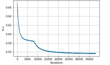
We applied this procedure to several relevant states, where the most significant examples are already given in the main text (see Table I in the main text). We now want to give the explicit forms of those states and also mention the results obtained for some further example states:
First, we considered Dicke states. These are entangled states, which were first investigated by R. H. Dicke in 1954 36. Symmetric Dicke states are of the form
| (57) |
with denoting the number of particles and the number of excitations. The notation describes a permutation of the qubits, where the sum runs over all possible permutations. Hence, for excitations and qubits we have
| (58) |
Dicke states with only excitation are called W states k-entanglement1. Here we found improved witnesses for
| (59) |
and
| (60) |
Note, that there also exist other works presenting witnesses specially tailored to Dicke states Bergmann. Still, as these are quite common states it is sensible to demonstrate the performance of the OSD witnesses also on these examples.
Further, we applied our algorithms to a three-qubit uniform hypergraph state given by 1404.6492:
| (61) | ||||
| (62) |
where the second expression is obtained, performing a Hadamard transformation of the third qubit.
Additionally, the four-qubit singlet state is given by rev5; four-qubit:
| (63) |
We also applied our algorithms to the state , which is a so-called comb monotone state comb. It is a maximally entangled state for certain entanglement measures and is defined as
| (64) |
We could improve the visibility for this state from to .
Appendix D Appendix D: Analytical approach
Since the choice of the operator so far only relies on numerical optimization where the computational effort may grow with the system size, we will give now an additional approach to choose based on analytical updates only.
First, considering the OSCs of the optimized operator found by the numerical algorithms, we find that for the three-qubit case, all OSCs are equal for all bipartitions: and . This gives rise to the idea to choose to be a GHZ-type operator as mentioned in the main text: . The four-level three-particle GHZ state does not only fulfill this condition on the OSCs but also is an absolutely maximally entangled (AME) state and hence a good candidate to construct an entanglement witness.
There are two ways to interpret this structure of the operator . For one thing, we can take it as a pure four-level three-particle (GHZ) state, where the vector of dimension four corresponds to an operator of dimension two. For the other thing this is the same as taking the projector of a pure two-level three-particle state and assigning the basis to it. In the following we will stay with the latter interpretation and now, having a rough idea how the structure of the optimized operator may look like, we introduce an update rule for the choice of the basis operators .
Note that in the latter interpretation, we mainly use the knowledge of the structure to define a starting point for our updates. To derive the update rules we may use a more general decomposition of the operator than the one given above. Therefore, we decompose , chosen as a projector of a GHZ state, in the following way:
| (66) |
with some arbitrary hermitian orthonormal bases , and and coefficients . Then the OSCs are defined by the coefficients , which means that updating the operators leaves the OSCs unchanged. Now, we will show how to choose the such that the expectation value of for the target state is maximized. First, consider:
| (67) |
In the following, we want to perform an orthogonal transformation on the operators . Starting with , we have:
| (68) | ||||
| (69) | ||||
| (70) | ||||
| (71) | ||||
| (72) |
In the third step we defined and in the last step we made use of the fact that the trace of some operator multiplied with an orthonormal operator is always maximized by the sum of its singular values . This shows that if is the singular value decomposition of , then the optimal transformation is given by . We proceed analogously for and , and step by step update the operators . For typical examples of three qubits, after roughly 20 iterations the expectation value converges to a maximum.
It is to mention that if the expectation value converges, the trace of the operator and therefore also must converge. Hence, also the visibility for white noise
| (73) |
converges. Still, as we do not renormalize the operator here, in general it might happen that the visibility is not monotone and therefore does not converge to the optimal value, however, for all examples considered here the visibility is monotone as well and thus we find minima for the visibility, too. Further, we stress that these updates are more general than simple local unitary transformations since already for qubits an orthogonal transformation including the identity may change the eigenvalues and the trace of the operator . Therefore, using this method, we indeed find new entanglement witnesses (not only rotated ones).
Since the coefficients are fixed during the optimization, the remaining question is how to choose them in a clever way, which results in the question how to choose the initial operator . Indeed, taking , where and decomposing it into some arbitrary bases , and to obtain the coefficients will, after updating the operators, give an OSD witness with visibility for the three-qubit W state and for the hypergraph state. Thus, we can improve the fidelity witness by only performing a few analytically chosen updates on , while for the three-qubit hypergraph state we even reach the same visibility as obtained by the numerical algorithm.
There are two remarks in order: First, one could also choose to built . This gives the same result for the hypergraph state, but a worse one for the W state. The reason is that this method can easily get stuck in local optima. So it is sensible to try out different starting operators . Still, taking AME states, or states with evenly distributed OSCs turn out to give good results. Second, we can do the same procedure for more than three qubits. Taking the projector of the four- or five-qubit GHZ state as starting operator, we can improve the visibility for the four-qubit hypergraph state with one big hyperedge from to and for five qubits from to . Hence, we introduced a method based on purely analytical steps, which allows us to find OSD witnesses with better visibility than fidelity witnesses and is also feasible for larger systems.
Appendix E Appendix E: Estimating multipartite entanglement monotones
In this appendix we will show how specific entanglement monotones for genuine multiparticle entanglement can be lower bounded via OSD witnesses.
First, considering a bipartite entanglement measures , we can define the corresponding genuine multipartite entanglement (GME) measure for pure states as
| (74) |
where denotes all possible bipartitions of observe2. This can then be extended to mixed states via the convex roof construction, , where the infimum runs over all possible decompositions of the mixed state .
Suppose that the dimension of the multipartite system under the bipartition is with . An arbitrarily chosen Hermitian operator in this multipartite system has its OSD under the bipartition as
| (75) |
where are the OSCs in decreasing order for the bipartition . As explained in the main text, if we define then
| (76) |
is a witness for GME. In the following, we also define . Similarly to Appendix B, one can now obtain lower bounds of GME measures based on the GME witness in Eq. (76).
Theorem 4. Consider an entanglement measure for bipartite states, such that we have for each bipartition
| (77) |
where is the Schmidt decomposition of the multiparticle state for the bipartition . We define the function as
| (78) |
where denotes the dependence on the underlying dimension. Then, let be the convex-hull of for . If is a monotonously decreasing function of and , and is a monotonously increasing convex function, then for an arbitrary -partite mixed state the bound
| (79) |
holds.
Proof. Assume that is the optimal decomposition for to achieve the infimum of . Then we have . For any possible bipartition , we can calculate of each as , where is the vector containing the Schmidt coefficients of under the bipartition . Then we have
| (80) | |||||
where we have used
| (81) |
based on Lemma 1 in Appendix B and the fact that is a monotonously decreasing function of and . Thus, we have that
| (82) |
where we have used is a monotonously increasing convex function.
Corollary 5. Similar to Appendix B and based on Theorem 4, we can obtain improved experimentally accessible lower bounds for GME measures, such as CREN of GME , the concurrence of GME , the G-concurrence of GME , and the geometric measure of GME . The bounds are given by
| (83a) | |||
| (83b) | |||
| (83c) | |||
| (83d) | |||
where . If we choose , the results of Eqs. (83a)-(83d) reduce to the results of Theorems 1-4 in Ref. observe2, respectively.
References
- (1) F. Arute, K. Arya, R. Babbush, D. Bacon, J. C. Bardin, R. Barends, R. Biswas, S. Boixo, F. G. S. L. Brandao, D. A. Buell, B. Burkett, Y. Chen, Z. Chen, B. Chiaro, R. Collins, W. Courtney, A. Dunsworth, E. Farhi, B. Foxen, A. Fowler, C. Gidney, M. Giustina, R. Graff, K. Guerin, S. Habegger, M. P. Harrigan, M. J. Hartmann, A. Ho, M. Hoffmann, T. Huang, T. S. Humble, S. V. Isakov, E. Jeffrey, Z. Jiang, D. Kafri, K. Kechedzhi, J. Kelly, P. V. Klimov, S. Knysh, A. Korotkov, F. Kostritsa, D. Landhuis, M. Lindmark, E. Lucero, D. Lyakh, S. Mandrà, J. R. McClean, M. McEwen, A. Megrant, X. Mi, K. Michielsen, M. Mohseni, J. Mutus, O. Naaman, M. Neeley, C. Neill, M. Y. Niu, E. Ostby, A. Petukhov, J. C. Platt, C. Quintana, E. G. Rieffel, P. Roushan, N. C. Rubin, D. Sank, K. J. Satzinger, V. Smelyanskiy, K. J. Sung, M. D. Trevithick, A. Vainsencher, B. Villalonga, T. White, Z. J. Yao, P. Yeh, A. Zalcman, H. Neven, and J. M. Martinis, Quantum supremacy using a programmable superconducting processor, Nature 574, 505 (2019).
- (2) S.-K. Liao, W.-Q. Cai, W.-Y. Liu, L. Zhang, Y. Li, J.-G. Ren, J. Yin, Q. Shen, Y. Cao, Z.-P. Li, F.-Z. Li, X.-W. Chen, L.-H. Sun, J.-J. Jia, J.-C. Wu, X.-J. Jiang, J.-F. Wang, Y.-M. Huang, Q. Wang, Y.-L. Zhou, L. Deng, T. Xi, L. Ma, T. Hu, Q. Zhang, Y.-A. Chen, N.-L. Liu, X.-B. Wang, Z.-C. Zhu, C.-Y. Lu, R. Shu, C.-Z. Peng, J.-Y. Wang, and J.-W. Pan, Satellite-to-ground quantum key distribution, Nature 549, 43 (2017).
- (3) D. P. Nadlinger, P. Drmota, B. C. Nichol, G. Araneda, D. Main, R. Srinivas, D. M. Lucas, C. J. Ballance, K. Ivanov, E. Y.-Z. Tan, P. Sekatski, R. L. Urbanke, R. Renner, N. Sangouard, and J.-D. Bancal, Experimental quantum key distribution certified by Bell’s theorem, Nature 607, 682 (2022).
- (4) W. Zhang, T. van Leent, K. Redeker, R. Garthoff, R. Schwonnek, F. Fertig, S. Eppelt, W. Rosenfeld, V. Scarani, C. C.-W. Lim, and H. Weinfurter, A device-independent quantum key distribution system for distant users, Nature 607, 687 (2022).
- (5) S. Ebadi, T. T. Wang, H. Levine, A. Keesling, G. Semeghini, A. Omran, D. Bluvstein, R. Samajdar, H. Pichler, W. W. Ho, S. Choi, S. Sachdev, M. Greiner, V. Vuletić, and M. D. Lukin, Quantum phases of matter on a 256-atom programmable quantum simulator, Nature 595, 227 (2021).
- (6) D. Gross, Y.-K. Liu, S. T. Flammia, S. Becker, J. Eisert, Quantum state tomography via compressed sensing, Phys. Rev. Lett. 105, 150401 (2010).
- (7) M. Cramer, M. B. Plenio, S. T. Flammia, R. Somma, D. Gross, S. D. Bartlett, O. Landon-Cardinal, D. Poulin, and Y.-K. Liu, Efficient quantum state tomography, Nat. Commun. 1, 149 ( 2010).
- (8) H. Y. Huang, R. Kueng, and J. Preskill, Predicting many properties of a quantum system from very few mea- surements, Nat. Phys. 16, 1050 (2020).
- (9) H. C. Nguyen, J. L. Bönsel, J. Steinberg, O. Gühne, Optimizing shadow tomography with generalized measurements, Phys. Rev. Lett. 129, 220502 (2022).
- (10) J. Cotler, F. Wilczek, Quantum Overlapping Tomography, Phys. Rev. Lett. 124, 100401 (2020).
- (11) N. Yu, T.-C. Wei, Learning marginals suffices, arXiv:2303.08938.
- (12) N. Brunner, D. Cavalcanti, S. Pironio, V. Scarani, S. Wehner, Bell nonlocality, Rev. Mod. Phys. 86, 419 (2014).
- (13) R. Uola, A. C. S. Costa, H. Chau Nguyen, O. Gühne, Quantum Steering, Rev. Mod. Phys. 92, 15001 (2020).
- (14) R. Horodecki, P. Horodecki, M. Horodecki, and K. Horodecki, Quantum entanglement, Rev. Mod. Phys. 81, 865 (2009).
- (15) O. Gühne, and G. Tóth, Entanglement detection, Phys. Rep. 474, 1 (2009).
- (16) N. Friis, G. Vitagliano, M. Malik, and M. Huber, Entanglement certification from theory to experiment, Nat. Rev. Phys. 1, 72 (2019).
- (17) S. Gharibian, Strong NP-hardness of the quantum separability problem, Quantum Inf. Comput. 10, 343 (2010).
- (18) M. A. Nielsen, and I. L. Chuang, Quantum Computation and Quantum Information, Cambridge University Press, Cambridge (2000).
- (19) M. Curty, M. Lewenstein, and N. Lütkenhaus, Entanglement as precondition for secure quantum key distribution, Phys. Rev. Lett. 92, 217903 (2004).
- (20) L. Pezzé and A. Smerzi, Entanglement, Non-linear Dynamics, and the Heisenberg Limit Phys. Rev. Lett. 102, 100401 (2009).
- (21) M. Bourennane, M. Eibl, C. Kurtsiefer, S. Gaertner, H. Weinfurter, O. Gühne, P. Hyllus, D. Bruß, M. Lewenstein, and A. Sanpera, Experimental Detection of Multipartite Entanglement Using Witness Operators, Phys. Rev. Lett. 92, 087902 (2004).
- (22) G. Tóth, Entanglement witnesses in spin models, Phys. Rev. A 71, 010301(R) (2005).
- (23) B. M. Terhal, A Family of Indecomposable Positive Linear Maps based on Entangled Quantum States, Linear Algebra Appl. 323, 61 (2000).
- (24) M. Lewenstein, B. Kraus, J. I. Cirac, and P. Horodecki, Optimization of entanglement witnesses, Phys. Rev. A 62, 052310 (2000).
- (25) O. Gühne, M. Mechler, G. Tóth, and P. Adam, Entanglement criteria based on local uncertainty relations are strictly stronger than the computable cross norm criterion, Phys. Rev. A 74, 010301 (2006).
- (26) M. Piani and C. Mora, Class of positive-partial-transpose bound entangled states associated with almost any set of pure entangled states, Phys. Rev. A 75, 012305 (2007).
- (27) D. Chruściński and G. Sarbicki, Entanglement witnesses: construction, analysis and classification, J. Phys. A: Math. Theor. 47, 483001 (2014).
- (28) A. Asadian, P. Erker, M. Huber, and C. Klöckl, Heisenberg-Weyl Observables: Bloch vectors in phase space, Phys. Rev. A 94, 010301(R) (2016).
- (29) J. Shang, A. Asadian, H. Zhu, and O. Gühne, Enhanced entanglement criterion via symmetric informationally complete measurements, Phys. Rev. A 98, 022309 (2018).
- (30) M. Weilenmann, B. Dive, D. Trillo, E. A. Aguilar, and M. Navascués, Entanglement Detection beyond Measuring Fidelities, Phys. Rev. Lett. 124, 200502 (2020); Erratum: Phys. Rev. Lett. 125, 159903 (2020).
- (31) O. Gühne, Y. Mao, and X.-D. Yu, Geometry of Faithful Entanglement, Phys. Rev. Lett. 126, 140503 (2021).
- (32) X.-L. Wang, L.-K. Chen, W. Li, H.-L. Huang, C. Liu, C. Chen, Y.-H. Luo, Z.-E. Su, D. Wu, Z.-D. Li, H. Lu, Y. Hu, X. Jiang, C.-Z. Peng, L. Li, N.-L. Liu, Y.-A. Chen, C.-Y. Lu, and J.-W. Pan, Experimental ten-photon entanglement, Phys. Rev. Lett. 117, 210502 (2016).
- (33) X.-C. Yao, T.-X. Wang, P. Xu, H. Lu, G.-S Pan, X.-H. Bao, C.-Z. Peng, C.-Y. Lu, Y.-A. Chen, J.-W. Pan, Observation of eight-photon entanglement, Nature Photon. 6, 225-228 (2012).
- (34) Y.-F. Huang, B.-H. Liu, L. Peng, Y.-H. Li, L. Li, C.-F. Li and G.-C. Guo, Experimental generation of an eight-photon Greenberger-Horne-Zeilinger state, Nature Commun. 2, 546 (2011).
- (35) M. A. Nielsen, Quantum information theory,Ph.D. thesis, University of New Mexico, Albuquerque, (1998).
- (36) M. A. Nielsen, C. M. Dawson, J. L. Dodd, A. Gilchrist, D. Mortimer, T. J. Osborne, M. J. Bremner, A. W. Harrow, and A. Hines, Quantum dynamics as a physical resource, Phys. Rev. A 67, 052301 (2003).
- (37) D. Cariello, Separability for Weak Irreducible matrices, Quantum Inf. Comput. 14, 1308 (2014).
- (38) D. Cariello, Analytical techniques on multilinear problems, PhD thesis, Universidad Complutense de Madrid, Madrid, (2017).
- (39) N. Johnston, http://www.njohnston.ca/2014/06/whatthe-operator-schmidt-decompositiontells-us-about-entanglement/.
- (40) G. De las Cuevas, T. Drescher, and T. Netzer, Separability for mixed states with operator Schmidt rank two, Quantum 3, 203 (2019).
- (41) R. Mansuroglu, A. Adil, M. J. Hartmann, Z. Holmes, and A. T. Sornborger, Quantum Tensor Product Decomposition from Choi State Tomography, arXiv:2402.05018v1
- (42) J. Eisert, and H. J. Briegel, Schmidt measure as a tool for quantifying multiparticle entanglement, Phys. Rev. A 64, 022306 (2001).
- (43) B. M. Terhal, and P. Horodecki, Schmidt number for density matrices, Phys. Rev. A 61, 040301(R) (2000).
- (44) A. Sanpera, D. Bruß, and M. Lewenstein, Schmidt number witnesses and bound entanglement, Phys. Rev. A 63, 050301(R) (2001).
- (45) N. Johnston, and D. W. Kribs, Duality of Entanglement Norms, Houston J. Math. 41(3), 831-847 (2015).
- (46) M. Horodecki, P. Horodecki, and R. Horodecki, Separability of mixed states: necessary and sufficient conditions, Phys. Lett. A 223, 1-8 (1996).
- (47) A. Peres, Separability criterion for density matrices, Phys. Rev. Lett. 77, 1413 (1996).
- (48) K. Życzkowski, P. Horodecki, A. Sanpera, and M. Lewenstein, Volume of the set of separable states, Phys. Rev. A 58, 883 (1998).
- (49) G. Vidal, and R. F. Werner, Computable measure of entanglement, Phys. Rev. A 65, 032314 (2002).
- (50) S. Lee, D.-P. Chi, S.-D. Oh, and J. Kim, Convex-roof extended negativity as an entanglement measure for bipartite quantum systems, Phys. Rev. A 68, 062304 (2003).
- (51) C. H. Bennett, D. P. DiVincenzo, J. A. Smolin, and W. K. Wootters, Mixed-state entanglement and quantum error correction, Phys. Rev. A 54, 3824-3851 (1996).
- (52) S. Hill, and W. K. Wootters, Entanglement of a Pair of Quantum Bits, Phys. Rev. Lett. 78, 5022 (1997).
- (53) W. K. Wootters, Entanglement of formation of an arbitrary state of two qubits, Phys. Rev. Lett. 80, 2245 (1998).
- (54) K. Audenaert, F. Verstraete, and B. De Moor, Variational characterizations of separability and entanglement of formation, Phys. Rev. A 64, 052304 (2001).
- (55) P. Rungta, V. Buzek, C. M. Caves, M. Hillery, and G. J. Milburn, Universal state inversion and concurrence in arbitrary dimensions, Phys. Rev. A 64, 042315 (2001).
- (56) P. Badziag, P. Deuar, M. Horodecki, P. Horodecki, and R. Horodecki, Concurrence in arbitrary dimensions, J. Mod. Opt. 49, 1289 (2002).
- (57) A. Uhlmann, Roofs and convexity, Entropy 12, 1799 (2010).
- (58) G. Gour, Family of concurrence monotones and its applications, Phys. Rev. A 71, 012318 (2005).
- (59) H. Fan, K. Matsumoto, and H. Imai, Quantify entanglement by concurrence hierarchy, J. Phys. A 36, 4151 (2003).
- (60) H. Barnum, and N. Linden, Monotones and invariants for multi-particle quantum states, J. Phys. A 34, 6787 (2001).
- (61) T.-C. Wei, and P. M. Goldbart, Geometric measure of entanglement and applications to bipartite and multipartite quantum states, Phys. Rev. A 68, 042307 (2003).
- (62) T.-C. Wei, J. B. Altepeter, P. M. Goldbart, and W. J. Munro, Measures of entanglement in multipartite bound entangled states, Phys. Rev. A 70, 022322 (2004).
- (63) K. Chen, S. Albeverio, and S.-M. Fei, Concurrence of Arbitrary Dimensional Bipartite Quantum States, Phys. Rev. Lett. 95, 040504 (2005).
- (64) O. Rudolph, Further Results on the Cross Norm Criterion for Separability, Quantum Inf. Process. 4, 219 (2005).
- (65) K. Chen and L.-A. Wu, A matrix realignment method for recognizing entanglement, Quantum Inf. Comput. 3, 193 (2003).
- (66) C. Lancien, O. Gühne, R. Sengupta, and M. Huber, Relaxations of separability in multipartite systems: Semidefinite programs, witnesses and volumes, J. Phys. A: Math. Theor. 48, 505302 (2015).
- (67) A. Acín, D. Bruß, M. Lewenstein, and A. Sanpera, Classification of Mixed Three-Qubit States, Phys. Rev. Lett. 87, 040401 (2001).
- (68) O. Gühne, M. Cuquet, F. E. S. Steinhoff, T. Moroder, M. Rossi, D. Bruß, B. Kraus, and C. Macchiavello, Entanglement and nonclassical properties of hypergraph states, J. Phys. A: Math. Theor. 47, 335303 (2014).
- (69) O. Gühne, and M. Seevinck, Separability criteria for genuine multiparticle entanglement, New J. Phys. 12, 053002 (2010).
- (70) C. Zhang, S. Yu, Q. Chen, and C. H. Oh, Detecting and Estimating Continuous-Variable Entanglement by Local Orthogonal Observables, Phys. Rev. Lett. 111, 190501 (2013).
- (71) B. Jungnitsch, T. Moroder, and O. Gühne, Taming Multiparticle Entanglement, Phys. Rev. Lett. 106, 190502 (2011).
- (72) N. Ganguly, S. Adhikari, A. S. Majumdar, and J. Chatterjee, Entanglement Witness Operator for Quantum Teleportation, Phys. Rev. Lett. 107, 270501 (2011).
- (73) R. O. Vianna, and A. C. Doherty, Distillability of Werner states using entanglement witnesses and robust semidefinite programs, Phys. Rev. A 74, 052306 (2006).
- (74) M. Huber, and J. I. de Vicente, Structure of Multidimensional Entanglement in Multipartite Systems, Phys. Rev. Lett. 110, 030501 (2013).
- (75) L. Bulla, M. Pivoluska, K. Hjorth, O. Kohout, J. Lang, S. Ecker, S. P. Neumann, J. Bittermann, R. Kindler, M. Huber, M. Bohmann, and R. Ursin, Nonlocal Temporal Interferometry for Highly Resilient Free-Space Quantum Communication, Phys. Rev. X 13, 021001 (2023).
- (76) S. T. Flammia, and Y.-K. Liu, Direct Fidelity Estimation from Few Pauli Measurements, Phys. Rev. Lett. 106, 230501 (2011).
- (77) S. Morelli, H. Yamasaki, M. Huber, and A. Tavakoli, Entanglement Detection with Imprecise Measurements, Phys. Rev. Lett. 128, 250501 (2022).
- (78) S. Denker, Characterizing multiparticle entanglement using the Schmidt decomposition of operators, Springer 2023
- (79) S. Liu, Q. He, M. Huber, O. Gühne, and G. Vitagliano, Characterizing Entanglement Dimensionality from Randomized Measurements, PRX Quantum 4, 020324 (2023).
- (80) N. Wyderka and A. Ketterer, Probing the Geometry of Correlation Matrices with Randomized Measurements, PRX Quantum 4, 020325 (2023).
- (81) C. Zhang, S. Yu, Q. Chen, H. Yuan, and C. H. Oh, Evaluation of entanglement measures by a single observable, Phys. Rev. A 94, 042325 (2016).
- (82) C. H. Bennett, D. P. DiVincenzo, T. Mor, P. W. Shor, J. A. Smolin and B. M. Terhal, Unextendible Product Bases and Bound Entanglement, Phys. Rev. Lett. 82, 5385 (1999).
- (83) R. H. Dicke, Coherence in Spontaneous Radiation Processes, Phys. Rev. 93, 99 (1954).
- (84) W. Dür, G. Vidal, and J. I. Cirac, Three qubits can be entangled in two inequivalent ways, Phys. Rev. A 62, 062314 (2000).
- (85) M. Bergmann, and O. Gühne, Entanglement criteria for Dicke states, J. Phys. A: Math. Theor. 46, 385304 (2013).
- (86) H. Weinfurter, and M. Żukowski, Four-photon entanglement from down-conversion, Phys. Rev. A 64, 010102(R) (2001).
- (87) B. Kraus, Entanglement properties of quantum states and quantum operations, PhD thesis, Universität zu Innsbruck (2003).
- (88) H. J. Briegel, and R. Raussendorf, Persistent Entanglement in Arrays of Interacting Particles, Phys. Rev. Lett. 86, 910 (2001).
- (89) Y. Dai, Y. Dong, Z. Xu, We. You, C. Zhang, and O. Gühne, Experimentally Accessible Lower Bounds for Genuine Multipartite Entanglement and Coherence Measures, Phys. Rev. Applied 13, 054022 (2020).