Surface roughness induced stress concentration

1 Introduction

Almost all tribology applications involves surface roughnessrev1; rev2; rev3; rev4; Carp. All surfaces of solids have roughness on many length scalesMRS1; MRS2; MRS3; MRS4; MRS5. When an elastic body is deformed the stress at the surface will vary strongly with the position on the surface, and may take values much higher than the applied stress, or the stress which would prevail if the surface would be perfectly smooth. The points where the stress is high may act as crack nucleation centers. In many practical applications bodies are exposed to deformations which fluctuate in time and after many stress fluctuation cycles the body could breakup (fracture). This is denoted as fatigue failure.

Silica glass is a good example for the influence of stress concentration at surface defects on its tensile strengthplast. Imperfections of the glass, such as surface scratches, have a great effect on the strength of glass. Thus silica glass plates typically have a tensile strength of $\sim 7\ {\rm MPa}$, but the theoretical upper bound on its strength is orders of magnitude higher: $\sim 17\ {\rm GPa}$. This high value is due to the strong chemical Si-O bonds of silicon dioxide. The probability to find large defects decreases as the size of an object decreases. This is well known for silica glass. Thus, glass fibers are typically 200-500 times stronger than for macroscopic glass plates.

Several different empirical equations have been presented for how to determine stress concentration at rough surfacesemp1; emp2. Two of them involve maximum height parameters such as $R_{z}$ (which I have denoted $h_{1z}$ in Ref. h1z) which is determined mainly by the longest wavelength roughness components (which have the largest amplitudes), and which will fluctuate strongly from one measurement to another (see Ref. h1z; press). However, most surfaces have self-affine fractal surface roughness with a fractal dimension $D_{\rm f}>2$ (or Hurst exponent $H<1$)PT; add2; add3. In these cases the ratio between the height and the wavelength of a roughness component increases as the wavelength decrease, i.e., the roughness becomes sharper at short lengthscale. Thus, one cannot neglect the short wavelength roughness when calculating the stress concentration factor.

In this paper I will derive the probability distribution of surface stress for randomly rough surfaces, and show how it can be used to estimate stress concentration factors. I will show that the maximum stress is proportional to the root-mean-square (rms) surface slope. I present numerical simulation results for height topographies and stress maps. This is the third paper where I study statistical properties of randomly rough surfaces with applications. The earlier papers focused on maximum height parameters with application to pressure fitspress; h1z.

2 Randomly rough surfaces

All surfaces of solids have surface roughness, and many surfaces exhibit self-affine fractal behavior. This implies that if a surface area is magnified new (shorter wavelength) roughness is observed which appears very similar to the roughness observed at smaller magnification, assuming the vertical coordinate is scaled with an appropriate factor.

The roughness profile $z=h({\bf x})$, where ${\bf x}=(x,y)$, of a surface can be written as a sum of plane waves ${\rm exp}(i{\bf q}\cdot{\bf x})$ with different wave vectors ${\bf q}$. The wavenumber $q=|{\bf q}|=2\pi/\lambda$, where $\lambda$ is the wavelength of one roughness component. The most important property of a rough surface is its power spectrum which can be written as

$$C({\bf q})={1\over(2\pi)^{2}}\int d^{2}x\ \langle h({\bf x})h({\bf 0})\rangle e^{i{\bf q}\cdot{\bf x}}$$

$(1)$

where $\langle..\rangle$ stands for ensemble averaging. Defining

$$h({\bf q})={1\over(2\pi)^{2}}\int d^{2}x\ h({\bf x})e^{-i{\bf q}\cdot{\bf x}}$$

$(2)$

$$h({\bf x})=\int d^{2}q\ h({\bf q})e^{i{\bf q}\cdot{\bf x}}$$

$(3)$

one can show that (see Appendix A):

$$C({\bf q})={(2\pi)^{2}\over A_{0}}\langle h({\bf q})h(-{\bf q})\rangle$$

$(4)$

where $A_{0}$ is the surface area. Assuming that the surface has isotropic statistical properties, $C({\bf q})$ depends only on the magnitude $q$ of the wave vector. A self affine fractal surface has a power spectrum $C(q)\sim q^{-2(1+H)}$ (where $H$ is the Hurst exponent related to the fractal dimension $D_{\rm f}=3-H$), which is a is a strait line with the slope $-2(1+H)$ when plotted on a log-log scale. Most solids have surface roughness with the Hurst exponent $0.7<H<1$ (see Ref. PT; add2; add3).

For randomly rough surfaces, all the (ensemble averaged) information about the surface is contained in the power spectrum $C({\bf q})$. For this reason the only information about the surface roughness which enter in contact mechanics theories (with or without adhesion) is the function $C({\bf q})$. Thus, the (ensemble averaged) area of real contact, the interfacial stress distribution and the distribution of interfacial separations, are all determined by $C({\bf q})$Persson2; Prodanov; Carbone1.

Note that moments of the power spectrum determines standard quantities which are output of most topography instruments and often quoted. Thus, for example, the mean-square roughness amplitude

$$h_{\rm rms}^{2}=\langle h^{2}\rangle=\int d^{2}q\ C({\bf q})$$

$(5)$

and the mean-square slope

$$\xi^{2}=\langle(\nabla h)^{2}\rangle=\int d^{2}q\ q^{2}C({\bf q})$$

$(6)$

are easily obtained as integrals involving $C({\bf q})$. We will denote the root-mean-square (rms) roughness amplitude with $h_{\rm rms}$ and the rms slope with $\xi$. If $C(q)$ denote the angular average (in ${\bf q}$-space) of $C({\bf q})$ then from (6):

$$\xi^{2}=2\pi\int_{q_{0}}^{q_{1}}dq\ q^{3}C(q).$$

$(7)$

Assuming $C(q)=C_{0}q^{-2-2H}$ this gives

$$\xi^{2}=2\pi\int_{q_{0}}^{q_{1}}dq\ C_{0}q^{1-2H}$$

For $H=1$ this gives

$$\xi^{2}=2\pi\int_{q_{0}}^{q_{1}}dq\ C_{0}q^{-1}$$

If we write $q=q_{0}e^{\mu}$ and $\mu_{1}={\rm ln}(q_{1}/q_{0})$ this gives

$$\xi^{2}=2\pi\int_{1}^{\mu_{1}}d\mu\ C_{0}$$

which shows that each decade in length scale contribute equally to the rms slope when $H=1$. When $H<1$ the short wavelength roughness will be more important but in typical application $H$ is close to $1$ and we will assume this in the numerical study presented in Sec. 6.

Surfaces of bodies of engineering interest, e.g., a ball in a ball bearing or a cylinder in a combustion engine, have always a roll-off region for small wavenumbers $q$, because such bodies have some macroscopic shape, but are designed to be smooth at length scales smaller that the shape of the body. In these cases the roll-off wavelength is determined by the machining process, e.g., by the size of the particles in sand paper or on a grinding wheel. If the roll-off region matters in a particular application depends on the size of the relevant or studied surface area. Thus, if the lateral size $L$ is small the wavenumber $q=2\pi/L$ may be so large that it will fall in the region where the surface roughness power spectrum exhibit self-affine fractal scaling, and the roll-off region will not matter. We note that some natural surfaces, such as surfaces produced by brittle fracture, have fractal-like roughness on all length scales up to the linear size of the body.

3 Average stress concentration (approximate)

Consider a half-elliptic cavity (height $d_{0}$ and radius of curvature at the bottom $r_{0}$) on the surface of a rectangular elastic block. Assume that the block is elongated so the stress in the bulk far enough from the cavity is constant $\sigma_{xx}=\sigma_{0}$ while all other components of the stress tensor vanish. The local stress $\sigma_{xx}$ close to the tip of the cavity is denoted $S\sigma_{0}$, where the stress concentration factor (see Fig. 1) (see Ref. notch; Pet; SK) $S=1+2\surd G$ where $G=d_{0}/r_{0}$. We are interested in the enhancement factor $S$ for randomly rough surfaces where there are short wavelength roughness on top of longer wavelength roughness and so on, where the qualitative picture presented in Appendix B prevail.

Here we will calculate the mean stress concentration by replacing $d_{0}/r_{0}$ with

$$G=-\langle h({\bf x})\nabla^{2}h({\bf x})\rangle$$

$(8)$

where $\langle..\rangle$ denotes ensemble averaging.. This approach includes the roughness on all length scales (see Fig. 2). Since (8) is independent of the coordinate ${\bf x}$ we can average (8) over the $xy$-surface. Using (3) in (8) this gives

$$G={1\over A_{0}}\int d^{2}xd^{2}qd^{2}q^{\prime}\ q^{2}\langle h({\bf q})h({\bf q^{\prime}})\rangle e^{i({\bf q}+{\bf q^{\prime}})\cdot{\bf x}}$$

$$={(2\pi)^{2}\over A_{0}}\int d^{2}q\ q^{2}\langle h({\bf q})h(-{\bf q})\rangle$$

$(9)$

where we have used that

$$\delta({\bf q}+{\bf q^{\prime}})={1\over(2\pi)^{2}}\int d^{2}x\ e^{i({\bf q}+{\bf q^{\prime}})\cdot{\bf x}}$$

Using (4) we get from (9)

$$G=\int d^{2}q\ q^{2}C({\bf q})=\xi^{2}$$

where $\xi$ is the surface mean slope. Thus

$$S\approx 1+2\xi.$$

$(10)$

4 Average stress concentration (exact)

Assume that a rectangular block is elongated by the stress $\sigma_{0}$ (see Fig. 3). For a block with perfectly smooth surfaces the stress will be uniform in the block with $\sigma_{xx}=\sigma_{0}$ and the other stress components equal to zero. When the block has surface roughness the local stress at the surface could be much higher that the applied stress $\sigma_{0}$ in particular at crack-like defects. Here we will calculate the rms stress concentration

$$\sigma_{\rm rms}^{2}=\langle\left(\sigma_{xx}-\sigma_{0}\right)^{2}\rangle$$

We write

$$\sigma({\bf x})=\sigma_{xx}({\bf x})-\sigma_{0}$$

Using (3) and (see Appendix C)

$$\sigma({\bf q})=2\sigma_{0}qf({\bf q})h({\bf q})$$

where

$$f({\bf q})={q_{x}^{2}\over q^{2}}\left(1+\nu{q_{y}^{2}\over q^{2}}\right)$$

where $\nu$ is the Poisson ratio, gives

$$\langle\sigma^{2}\rangle={1\over A_{0}}\int d^{2}x\ \sigma^{2}({\bf x})$$

$$={2\pi\over A_{0}}\int d^{2}q\ q^{2}(2\sigma_{0})^{2}f^{2}({\bf q})\langle h({\bf q})h(-{\bf q}))\rangle$$

$$=\int d^{2}q\ q^{2}(2\sigma_{0})^{2}f^{2}({\bf q})C({\bf q})$$

$(11)$

If we assume roughness with isotropic statistic properties $C({\bf q})$ depends only on $q$ and in this case the angular integral in (11) can be performed analytically and we get (see Appendix C)

$$\langle\sigma^{2}\rangle=(2\sigma_{0})^{2}\xi^{2}g^{2}$$

where

$$g^{2}={1\over 8}\left(3+\nu+{3\over 16}\nu^{2}\right)$$

Thus the rms stress concentration

$$\sigma_{\rm rms}=2\xi g\sigma_{0},$$

$(12)$

In a typical case $\nu\approx 0.3$ giving $g\approx 0.64$ so (12) is consistent with (10).

5 Probability distribution of stress

For an infinite system the probability distribution of stresses $\sigma=\sigma_{xx}-\sigma_{0}$ will be a Gaussian (see Appendix D):

$$P(\sigma)={1\over(2\pi)^{1/2}\sigma_{\rm rms}}e^{-(\sigma/\sigma_{\rm rms})^{2}/2},$$

$(13)$

where $\sigma_{\rm rms}=2\xi g\sigma_{0}$. This equation imply that there will be arbitrary high local stresses at some points. However, for any finite system the probability to find very high stresses is small. We will now show how from (13) one can estimate the highest stress at the surface.

The stress probability distribution results from the fact that the stress is obtained by adding contributions to $P(\sigma)$ from each length scale with random phases. We have shown above that in a typical case where $H\approx 1$ each decade in length scale below the roll-off length scale gives approximately equal contributions to the rms slope and hence to $\sigma_{\rm rms}$. Hence there will $N\approx(\lambda_{\rm r}/\lambda_{1})^{2}$ important uncorrelated (because of the random phases) contributions to the probability distribution $P(\sigma)$ from the region $q_{r}<q<q_{1}$. The roll-off region correspond to $(\lambda_{0}/\lambda_{r})^{2}$ uncorrelated units so the total number of uncorrelated terms is $N\approx(\lambda_{\rm r}/\lambda_{1})^{2}(\lambda_{0}/\lambda_{\rm r})^{2}=(q_{1}/q_{0})^{2}$ which is the same as when no roll-off region exist. Note that this is very different from the probability distribution for surface heights where the region $q>q_{\rm r}$ gives a fixed number of uncorrelated terms independent of $q_{1}$ if $q_{1}/q_{\rm r}>>1$. The reason for this is that the height distribution $P(h)$ depends mainly on the longest wavelength surface roughness components, which have the largest amplitudes.

An estimation of the maximum stress $\sigma_{\rm max}$ can be obtained from the condition

$$\int_{\sigma_{\rm max}}^{\infty}d\sigma\ P(\sigma)\approx N^{-1}$$

$(14)$

Denoting $x=\sigma_{\rm max}/\sigma_{\rm rms}$ from (13) and (14) we get if $N>>1$:

$$x\approx\left[2{\rm ln}\left({N\over(2\pi)^{1/2}x}\right)\right]^{1/2}$$

$(15)$

In a typical case $\lambda_{\rm 0}=1\ {\rm cm}$ and $\lambda_{1}=1\ {\rm nm}$ giving $N=10^{14}$ and from (15) $x\approx 7.7$ and the maximum stress is $\sigma_{0}+\sigma_{\rm max}\approx(1+15.4\xi g)\sigma_{0}$. In a typical case $\xi\approx 1$ and the maximum local stress will be $\sim 10$ times bigger than the applied stress. We will consider the influence of plastic flow and crack formation on the roughness profile and the stress distribution in Sec. 7.

6 Numerical results

We will now discuss the relation between the maximum surface stress $\sigma_{\rm max}$ and the rms stress $\sigma_{\rm rms}=2\xi g\sigma_{0}$. No two surfaces have the same surface roughness, and $\sigma_{\rm max}$ will depend on the surface used. To take this into account we have generated surfaces (with linear size $L$) with different random surface roughness but with the same surface roughness power spectrum. That is, we use different realizations of the surface roughness but with the same statistical properties. For each surface size we have generated 60 rough surfaces using different set of random numbers. The surface roughness was generated as described in Ref. PT (appendix A) by adding plane waves with random phases $\phi_{\bf q}$ and with the amplitudes determined by the power spectrum:

$$h({\bf x})=\sum_{\rm q}B_{\bf q}e^{i({\bf q}\cdot{\bf x}+\phi_{\bf q})}$$

$(16)$

where $B_{\bf q}=(2\pi/L)[C({\bf q})]^{1/2}$. We assume isotropic roughness so $B_{\bf q}$ and $C({\bf q})$ only depend on the magnitude of the wavevector ${\bf q}$. The surface stress $\sigma_{0}+\sigma({\bf x})$ can be calculated from (C10) or can be generated directly using

$$\sigma({\bf x})=\sigma_{0}\sum_{\rm q}F_{\bf q}e^{i({\bf q}\cdot{\bf x}+\phi_{\bf q})}$$

$(17)$

where

$$F_{\bf q}=2qf({\bf q})B_{\rm q}=(2\pi/L)\left[4q^{2}f^{2}({\bf q})C({\bf q})\right]^{1/2}.$$

$(18)$

In the present numerical study we will assume that the surface roughness has isotropic statistical properties so that $C({\bf q})$ only depends on $q=|{\bf q}|$. However, even in this case the stress $\sigma_{xx}$ has anisotropic statistical properties because of the factor $f({\bf q})$ in (18). However, here we are only interested in comparing the prediction of (15) with the numerical theory, and for this it is enough to replace $f$ with its angular average value $1/2+\nu/8$ which we can consider as included in an effective $\sigma_{0}$. Thus we assume $f=1$ both in the numerical calculation and in (15) when comparing the theory with the numerical study.

We have used surfaces of square unit size, $L\times L$, with 7 different sizes, where $L$ increasing in steps of a factor of $2$ from $L=79\ {\rm nm}$ to $L=5.06\ {\rm\mu m}$, corresponding to increasing $N$ from $N=256$ to $N=16384$. The lattice constant $a\approx 0.309\ {\rm nm}$.

The longest wavelength roughness which can occur on a surface with size $L$ is $\lambda\approx L$ so when producing the roughness on a surface we only include the part of the power spectrum between $q_{0}<q<q_{1}$ where $q_{0}=2\pi/L$ and where $q_{1}$ is a short distance cut-off corresponding to atomic dimension (we use $q_{1}=1.4\times 10^{10}\ {\rm m^{-1}}$). This is illustrated in Fig. 4 which shows the different short wavenumber cut-off $q_{0}$ used.

We now study how the ratio $\sigma_{\rm max}/\sigma_{\rm rms}$ depends on the surface roughness power spectra. We will consider two cases where there is (a) no roll-off region in the power spectra and (b) where a roll-off region occur. Fig. 4 shows the surface roughness power spectra as a function of the wave number (log-log-scale) used in the calculations of the surface height profile for surfaces with the Hurst exponent $H=1$ without (a) and with (b) a roll-off region. Note that a vertical shift in power spectra in (b) has no influence on the ratio $\sigma_{\rm max}/\sigma_{\rm rms}$ since it correspond to scaling $C({\bf q})$ with some factor $s^{2}$, which is equivalent to scaling $h({\bf x})$ and hence $\sigma({\bf x})$ with the factor of $s$, which changes both $\sigma_{\rm max}$ and $\sigma_{\rm rms}$ with the same factor $s$, so the ratio $\sigma_{\rm max}/\sigma_{\rm rms}$ is unchanged.

Fig. 5 shows the cumulative probability for the ratio $\sigma_{\rm max}/\sigma_{\rm rms}$ between the height of the highest asperity (relative to the average surface plane) and the rms roughness amplitude for the power spectra shown in Fig. 4 without (a) and with (b) a roll-off region. Note that $\sigma_{\rm max}/\sigma_{\rm rms}$ depends on the system size in a very similar way for the case of no roll-off region and a roll-off region. This is very different from the roughness amplitude ratio $h_{\rm max}/h_{\rm rms}$ which is independent of the size of the surface area when no roll-off occur. For the case of a roll-off region the ratio $h_{\rm max}/h_{\rm rms}$ increases continuously with increasing roll-off region $q_{0}<q<q_{\rm r}$ as also observed for $\sigma_{\rm max}/\sigma_{\rm rms}$.

Fig. 6 shows the ratio $\sigma_{\rm max}/\sigma_{\rm rms}$ between the highest surface stress and the rms surface stress. as a function of the logarithm of the size of the unit $L$. The red and green lines are with and without a roll-off region in the power spectra, and the results are obtained after averaging over 60 realizations of the surface roughness. The blue line is the theory prediction using (15) with $N=(L/a)^{2}$ i.e. assuming that all the roughness components contribute equally.

We note that since $\sigma_{\rm rms}$ is an average over the whole surface area it is nearly identical for all the 60 realizations. This is clear if we plot the probability distribution of stresses as shown in Fig. 7. All 60 realizations gives nearly perfect Gaussian distributions with equal width (the rms width is $\sigma_{\rm rms}$).

Fig. 8 shows the (a) height topography $z=h(x,y)$ (where $h$ positive into the material) and (b) the surface stress distribution $\sigma(x,y)=\sigma_{xx}(x,y)-\sigma_{0}$ for the surface with $L=1.26\ {\rm\mu m}$ without a roll-off. The rms surface roughness $h_{\rm rms}=0.058$, the rms slope $\xi=0.823$, and the rms stress $\sigma_{\rm rms}=1.646\sigma_{0}$. Note on the average stress is high in the deep roughness wells (red area in both pictures).

Fig. 9 shows the same as in Fig. 8 but with roll-off. The rms surface roughness $h_{\rm rms}=0.058$ and the rms slope $\xi=10.86$. The large slope (and hence large $\sigma/\sigma_{0}$) is unphysical and result from the fact that the rms roughness amplitude was chosen the same for the power spectrum with and without roll-off. However, scaling $h(x,y)$ by a factor of $0.1$ gives a physical reasonable slope and this correspond to scaling the stress with the same factor of 0.1 which would give a similar stress variation as in the case of no roll-off.

Fig. 8 shows that the highest stress surface regions tend to occur at the bottom of the longest wavelength (large amplitude) roughness components. This support the empirical attempts to relate the stress concentration factor to maximum height parameters such as $R_{z}$. However, the treatment in Sec. 5 shows that the important parameter is the rms-slope and the range of roughness components which determines $N$ both of which can be obtained from the surface roughness power spectra.

7 Discussion

We have assumed that only elastic deformations occur in the solid. This is a good assumption as long as the applied stress $\sigma_{0}$ is small enough but in general one expect plastic flow and crack formation and propagation at the surface. Assume first that only plastic deformations occur (with the yield stress in tension $\sigma_{\rm Y}$). If the applied stress is larger than $\sim\sigma_{\rm Y}/10$ the local stress in some locations will be above the plastic yield stress in tension and plastic deformation is expected. But this plastic flow may occur only at short length scale (involving the short wavelength roughness), and since the yield stress may increase at short length scale the plastic deformations may be smaller than expected based on the macroscopic yield stress. (An increase in the yield stress at short length scales is well-known from indentation experiments where the penetration hardness $\sigma_{\rm P}\approx 3\sigma_{\rm Y}$ often increases as the indentation size decreases.size) If plastic deformation occur it will change the surface profile and reduce the local tensile stress so that it is at most the yield stress in tension $\sigma_{\rm Y}$. If one assume that the plastically deformed surface region does not change the stress in the regions which have not undergone plastic deformation, and if $\sigma_{\rm Y}$ is independent of the length scale, then the fraction of the surface which has undergone plastic deformation is determined by

$${A_{\rm pl}\over A_{0}}=\int_{\sigma_{\rm Y}-\sigma_{0}}^{\infty}d\sigma\ P(\sigma)$$

Next we consider the ideal case where no plastic deformations occur but only crack propagation (ideal brittle solid). The stress concentration at the surface resulting from the surface roughness can initiate crack growth. Here it is important to note that the deformation (and stress) field from a roughness component with the wavelength $\lambda$ will extend into the solid a distance $\sim\lambda/\pi$ [see (C45) and Appendix E] so when the crack has moved into the solid the distance $\sim\lambda/\pi$ it has already made use of all the elastic deformation energy associated with this roughness component. If it can propagate further depends on the elastic energy stored in the other longer roughness wavelength components. Hence in this case it is possible that a crack propagate only a finite distance into the solid. This could result in a network of surface cracks of finite depth as sometimes observed in experiments. Thus in Ref. Si it was found that when a sandblasted silica glass plate was thermally annealed a network of short cracks formed on the surface (see Fig. 13). This could be due to a tensile stress acting in a top layer of the silica plate due to the thermal contraction during cooling, which is stronger at the (colder) surface than inside the glass plate. For a similar glass plate which was not sandblasted a much smaller concentration of cracks was formed, as expected from theory due to a lower concentration of surface defects.

Here we present a simple dimensional analysis of how the surface stress generate cracks and plastic deformations. Consider a small crack at the surface of a solid exposed to a tensile stress. Except for an angular factor, of no importance here, the stress in the vicinity of the crack tip iscrack

$$\sigma\approx\sigma_{d}\left({d\over r}\right)^{1/2}$$

$(19)$

where $r$ is the distance from the crack tip, $d$ is the length of the crack and $\sigma_{d}$ is the tensile stress a distance $\sim d$ from the crack tip (note: $\sigma_{d}$ is larger than the applied stress $\sigma_{0}$ which occur far away from the crack tip). The critical length of the crack is determined by standard argumentsGriffith, namely $U^{\prime}(d)=0$ where $U(d)$ is the total energy. The reduction in the elastic energy induced by the crack

$$U_{\rm el}\approx-{1\over 2}\sigma\epsilon d^{2}L\approx-{1\over 2}{\sigma_{d}^{2}\over E}d^{2}L$$

where $d^{2}L$ is the volume where the deformation energy is reduced (see Fig. 10). The surface energy

$$U_{\rm area}=dL\gamma$$

where $\gamma$ is the energy per unit area to create the fracture surfaces. From $U^{\prime}(d)=0$ with $U=U_{\rm el}+U_{\rm area}$ we get the critical length $d=d^{*}$

$$d^{*}={E\gamma\over\sigma_{d}^{2}}$$

$(20)$

Fig. 11 shows the total energy $U(d)$ as a function of $d$. If $d<d^{*}$ no crack growth will occur while when $d>d^{*}$ unstable (accelerating) crack growth may occur. However, since the tensile stress decreases with increasing distance into the solid the crack will propagate only as long as the drop in the elastic energy is larger than the increase in the surface energy. We will now study this using a simple model.

The stress at the surface decay with the distance $z$ into the solid. As an example, assume that the stress $\sigma(z)$ decreases from $(1+\beta)\sigma_{0}$ to $\sigma_{0}$ with the distance $z$ according to

$$\sigma(z)=\left(1+\beta e^{-\alpha z}\right)\sigma_{0}$$

In this case (20) gives

$$d\left(1+\beta e^{-\alpha d}\right)^{2}=D$$

$(21)$

where the length parameter $D=E\gamma/\sigma_{0}^{2}$. In Fig. 12 we show the solution to (21) for $\beta=10$ and $1/\alpha=1\ {\rm\mu m}$ (red curve) and $10\ {\rm\mu m}$ (blue curve).

Suppose now that we slowly increase the external stress $\sigma_{xx}=\sigma_{0}$ until a crack-like defect (with the initial length $d_{1}$) start to grow. At this point we keep $\sigma_{0}$ fixed and study the time evolution of the crack length $d$. As $\sigma_{0}$ increases $D$ decreases from $\infty$ to some finite value $D$. Assume first $d_{1}>d_{\rm a}$. The crack cannot grow until we increased $\sigma_{0}$ so that $d(D)=d_{1}$. At this point the elastic energy stored in the vicinity of the crack tip is big enough to break the bonds and allow the crack to grow. However, as it growth ($d$ increases) Fig. 12 shows that a larger $D$, and hence smaller applied stress $\sigma_{0}$, is enough to grow the crack further. But since we keep $\sigma_{0}$ (and hence $D$) fixed the crack will accelerate resulting in a rapid catastrophic fracture of the solid. The same is true if the initial crack length is $d_{1}<d_{\rm c}$

Now assume $d_{\rm b}<d_{1}<d_{\rm a}$. The crack does not grow until $D$ has decreased so that $d(D)=d_{1}$. At this point the crack start to grow but now an increase in the crack length require a smaller $D$, and hence larger $\sigma_{0}$, i.e. there is not enough stored elastic energy to propagate the crack if $\sigma_{0}$ is kept constant. If we increase $\sigma_{0}$ the crack will grow but in a stable manner until the crack length reach $d=d_{\rm a}$ at which point fast (accelerated) growth occur again resulting in catastrophic failure of the body.

Finally, assume that $d_{\rm c}<d_{1}<d_{\rm b}$. In this case when $D$ has decreased (and the stress $\sigma_{0}$ has increased) so that $d(D)=d_{1}$ the crack length will increase initially in an accelerating way since the $d(D)$ curve has a positive slope at $d=d_{1}$. However, since $D>D_{\rm a}$, where $D_{\rm a}$ is the solution to $d(D)=d_{\rm a}$ the motion will slow down and stop somewhere in the region $d_{\rm b}<d_{1}<d_{\rm a}$. Here we have neglected kinetic effects i.e. we have assumed that there is not enough kinetic energy associated with the initial rapid crack tip motion to move over the “barrier” at $d=d_{\rm a}$. (Note: Linear elastic fracture mechanic theory predict that cracks have no inertiainert. Thus the crack will adjust its speed instantaneously to the driving force determined by the elastic energy stored in the solid in its vicinity. If the elastic deformation energy driving crack propagation is larger than the adiabatic fracture energy $\gamma$ then the additional energy is “dissipated” by creating surface roughness (and hence surface area) on the fracture surfaces, and by emission of elastic waves from the crack tip, and by other inelastic processes. However, see Ref. inertia.)

The discussions above assumes that no plastic deformations occur during crack propagation. For most solids, in particular metals, some plastic deformation (or other inelastic processes) will occur close to the crack tipplast; Irwin. One can determine the size $d_{\rm Y}$ of the region where plastic flow occur as follows: Plastic flow start when the tensile stress reaches $\sigma_{\rm Y}$. Using (19) we get

$$\sigma_{\rm Y}\approx\sigma_{d}\left({d\over d_{\rm Y}}\right)^{1/2}$$

or using (20)

$$d_{\rm Y}=\left({\sigma_{d}\over\sigma_{\rm Y}}\right)^{2}d={E\gamma\over\sigma_{\rm Y}^{2}}$$

$(22)$

If $d_{\rm Y}<<d$ then the crack theory presented above is valid but the surface energy $\gamma$ is not just the energy to break the bonds at the crack tip but must include the energy of plastic deformation (the crack surfaces are covered by thin films of plastically deformed material). If $d_{\rm Y}>d$ no crack propagation will occur but just local plastic deformation. For amorphous solids such as silica glass and amorphous silicon $d_{\rm Y}$ is typically a few ${\rm nm}$ while for metals $d_{\rm Y}\approx 10\ {\rm\mu m}$ or more (see Appendix F).

Similar ideas as discussed above have been presented in models of adhesive wear where big wear particles form by crack propagation in the large asperity contact regions, while small asperity contact regions deform plastically without generation of wear particlesRabin0; Rabin1; Rabin2; Moli2; Moli0; Moli1.

The stress concentration due to surface roughness can result in stress corrosionCic. Chemical bonds between atoms can be broken either by thermal fluctuations or by an applied force (stress). When the applied force is not high enough to break a bond the bond could still be broken by a large enough thermal fluctuationSzl. When the applied force increases the energy needed to overcome the barrier towards bond breaking decreases and the probability rate of (thermally assisted) bond breaking increases. This stress-aided, thermally activated process can result in the slow growth of surface cracks and to stress corrosion.

Stress corrosion cracking is the formation of cracks in a material through the simultaneous action of a tensile stress, temperature and a corrosive environment. Stress corrosion cracking has become one of the main reasons for the failure of steam generator tubing. The specific environment is of crucial importance, and only very small concentrations of certain highly active chemicals are needed to produce catastrophic cracking, often leading to devastating and unexpected failure.

Finally we note that the main driving force for the study of surface stress concentration is material fatigue which account for the majority of disastrous failure of mechanical devices e.g. airplanes. Fatigue damage of a component typically develop due to surface stress concentration originating from the surface topographyfat1; fat2. This result in the formation of crack-like defects which at some stage can propagate rapidly, possibly resulting in an unexpected catastrophic event.

Fatigue crack propagation in metals involves stress concentration and plastic deformations. Short wavelength roughness may be “smoothed” by plastic flow before a crack can nucleate and propagate because the elastic deformation energy density needed to propagate a crack increases as the crack size decreases.

It is remarkable that a solid can fail by crack propagation when exposed to a stress fluctuating in time (fatigue failure), but not (if the stress is small enough) when exposed to a static stress of the same magnitude as the amplitude of the oscillating stress. This indicate that some irreversible processes, not involving crack propagation, occur during the stress oscillations. For metals this likely involves point defects and dislocations which can form and move by the oscillating crack tip stress field, and which accumulate with increasing time in the region close to the crack tip and reduce the energy per unit area $\gamma$ to create new fracture surfacesfatigue. If $\gamma$ is reduced enough the crack can propagate even if for the original virgin solid this was not the case. For viscoelastic materials such as rubber the effective energy $\gamma$ to propagate a crack is smaller in an oscillating stress field because of viscoelasticityvisc1; visc2, and this explain why rubber wear, involving removing small rubber particles, occur during sliding (where the rubber surface is exposed to pulsating stresses from the countersurface asperities) while for a static contact with the same stress amplitude no (or negligible) crack propagation and wear particle formation occur.

Other applications of the theory presented above are to surface kineticsd3. The atoms in a stressed region on a solid surface have higher energy than in a non-stressed region. As a result less energy is needed to remove atoms from stressed surface regions. This may result in diffusion of atoms from stressed regions to less stressed surface regions. For a flat surface the surface stress is uniform (equal to $\sigma_{0}$) but for a surface with roughness the stress varies with the surface position, and theory shows that this may result in short wavelength roughness being smoothed by surface diffusion while long wavelength roughness may grow unstably. Similarly, evaporation-condensation is affected by the surface stress. Thus when the surface evolution is controlled by evaporation from or condensation to a surface, such that there is no net translation of the surface, the short wavelength roughness are smoothed by the evaporation/condensation process, whereas long wavelength roughness grow unstablyd3.

The theory in this paper is based on the small slope approximation. In Ref. d1 the results of the small slope approximation was compared to experiment and to FEM calculations for 1D wavy surfaces, and nearly perfect agreement with the theory was obtained for surfaces with the rms-slope $\sim 0.2$, where the maximum stress concentration factor was $S\approx 2$. Similarly, in Ref. add the theory prediction was found to be within $\sim 20\%$ of the FEM prediction even for a 1D wavy surface with the rms slope as large as $\sim 1$.

8 Summary and conclusion

When a body is exposed to external forces large local stresses may occur at the surface because of surface roughness. For randomly rough surfaces I calculate the probability distribution of surface stress in response to a uniform external tensile stress $\sigma_{0}$. I have shown that for randomly rough surfaces of elastic solids, the maximum local surface stress is given by $(1+s\xi)\sigma_{0}$, where typically $s\approx 10$. For most surfaces of engineering interest, when including all the surface roughness, the rms slope $\xi\approx 1$ giving maximal local tensile stresses of order $\sim 10\sigma_{0}$ or more.

I have presented numerical simulation results for the stress distribution $\sigma(x,y)$ and discussed the role of the stress concentration on plastic deformation and surface crack generation and propagation. The present study is important for many application and in particular for fatigue due to pulsating external forces, and to surface kinetics such as surface diffusion and evaporation/condensation phenomena.

Acknowledgments: I thank Jay Fineberg for discussions about crack inertia and R.O. Jones and M. Müser for discussions about chemical bonding in relation to Appendix F. I thank R. Carpick for comments on the text.

Funding: Open Access funding enabled and organized by Projekt DEAL. The authors have not disclosed any funding.

Conflict of interest: The author declare no conflict of interest in this study.

Appendix A: The power spectra

In Ref. PT (see also P; PJCP) we have derived (4) but for the readers convenience we repeat the derivation here. Because of translation invariance of the statistical properties of a randomly rough surface we can write (1) as

$$C({\bf q})={1\over(2\pi)^{2}}\int d^{2}x\ \langle h({\bf x}+{\bf x}^{\prime})h({\bf x}^{\prime})\rangle e^{i{\bf q}\cdot{\bf x}}$$

$(A1)$

Since (A1) is independent of ${\bf x}^{\prime}$ we can integrate over the ${\bf x}^{\prime}$-surface and divide by the nominal area $A_{0}$ to get

$$C({\bf q})={1\over(2\pi)^{2}}{1\over A_{0}}\int d^{2}xd^{2}x^{\prime}\ \langle h({\bf x}+{\bf x}^{\prime})h({\bf x}^{\prime})\rangle e^{i{\bf q}\cdot{\bf x}}$$

Using (3) and performing the ${\bf x}$ and ${\bf x}^{\prime}$ integrals and using that

$${1\over(2\pi)^{2}}\int d^{2}x\ e^{i({\bf q}+{\bf q^{\prime}})\cdot{\bf x}}=\delta({\bf q}+{\bf q^{\prime}})$$

we get

$$C({\bf q})={(2\pi)^{2}\over A_{0}}\int d^{2}q^{\prime}d^{2}q^{\prime\prime}\ \langle h({\bf q^{\prime}})h({\bf q^{\prime\prime}})\rangle$$

$$\times\delta({\bf q^{\prime}}+{\bf q})\delta({\bf q^{\prime}}+{\bf q^{\prime\prime}})$$

$$={(2\pi)^{2}\over A_{0}}\langle h({\bf q})h(-{\bf q})\rangle$$

Appendix B: Stress concentration factor

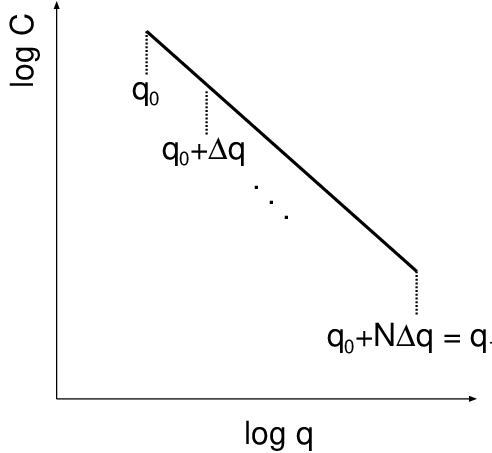
The stress at the tip of a surface “cavity” (or valley) is larger than the applied stress $\sigma_{0}$ by a factor $S=1+2\surd(d_{0}/r_{0})$ (see Fig. 1). But real surface have roughness on many length scales which we can formally consider as the sum of $N$ wavenumber regions as indicated in Fig. 14. If $S_{1}$ is the enhancement factor including only the roughness from the longest wavelength segment $q_{0}<q<q_{0}+\Delta q$ then when we add the roughness from the next roughness segment the enhancement becomes $S_{1}S_{2}$ and so on. If the segments are short then for each length scale $\surd(d/r)<<1$ and we get the total stress enhancement factor

$$S=(1+2\surd(d/r)\mid_{1})(1+2\surd(d/r)\mid_{2})..(1+2\surd(d/r)\mid_{N})$$

$$\approx 1+\sum_{n}2\surd(d/r)\mid_{n}$$

The qualitative picture underlying this approach is similar to the way multiscale roughness was taken into account in the study of fluid contact angles on randomly rough surfaces in Ref. fangle.

Appendix C: Stress–surface-roughness relation

Here we derive the relation between the stress $\sigma_{xx}({\bf x})=\sigma_{0}+\sigma({\bf x})$ and the surface roughness $z=h({\bf x})$. This problem has been studied before for a 1D roughness profile using the Airy stress functiond1 (see also d2 for another approach), but here we derive it for an arbitrary 2D surface roughness profile in the small slope approximation. The derivation presented here can be easily generalized to layered materialslayer.

To first order in $h^{\prime}_{x}$ and $h^{\prime}_{y}$ the normal unit vector to the surface $z=h(x,y)$ is given by (see Fig. 15):

$${\bf s}=\left(-h^{\prime}_{x},-h^{\prime}_{y},1\right).$$

Since the surface stress $\sigma_{ij}s_{j}$ must vanish we get

$$-h_{x}^{\prime}\sigma_{xx}-h^{\prime}_{y}\sigma_{xy}+\sigma_{xz}=0$$

$$-h_{x}^{\prime}\sigma_{yx}-h^{\prime}_{y}\sigma_{yy}+\sigma_{yz}=0$$

$$-h_{x}^{\prime}\sigma_{zx}-h^{\prime}_{y}\sigma_{zy}+\sigma_{zz}=0$$

Assuming that without the surface roughness the stress $\sigma_{xx}=\sigma^{0}_{xx}$ and $\sigma_{yy}=\sigma^{0}_{yy}$ are constant while all the other stress components vanish. This imply that with surface roughness all other stress components are already of first order in $h_{x}^{\prime}$ and $h_{y}^{\prime}$, and products such as $h_{x}^{\prime}\sigma_{xy}$ are of second order and can be neglected. Thus to first order in $h^{\prime}_{x}$ and $h^{\prime}_{y}$

$$-h^{\prime}_{x}\sigma^{0}_{xx}+\sigma_{xz}=0$$

$(C1)$

$$-h^{\prime}_{y}\sigma^{0}_{yy}+\sigma_{yz}=0$$

$(C2)$

$$\sigma_{zz}=0$$

$(C3)$

In what follows we will denote $\sigma_{xx}-\sigma^{0}_{xx}$ with just $\sigma_{xx}$ and similar for $\sigma_{yy}$. In this case all the components of the stress tensor $\sigma_{ij}$ will be of first order in $h^{\prime}_{x}$ and $h^{\prime}_{y}$. Since the stress tensor is already linear in $h_{x}^{\prime}$ and $h_{y}^{\prime}$ we can consider the surface of the solid as flat (no roughness) when calculating the elastic deformation field and the stress in the solid using the boundary conditions (C1)-(C3).

We write

$$h({\bf x})=\int d^{2}q\ h({\bf q})e^{i{\bf q}\cdot{\bf x}}$$

$(C4)$

so from (C1) the stress $\sigma_{xz}({\bf x},z)$ at the surface $z=0$ takes the form

$$\sigma_{xz}({\bf x},0)=\sigma^{0}_{xx}\int d^{2}q\ (iq_{x})h({\bf q})e^{i{\bf q}\cdot{\bf x}}$$

$(C5)$

and similar for $\sigma_{yz}({\bf x},0)$. If we define the vector ${\boldsymbol{\sigma}}=(\sigma_{xz},\sigma_{yz},\sigma_{zz})$ the boundary conditions (C1)-(C3) can be written as

$${\boldsymbol{\sigma}}=(h^{\prime}_{x}\sigma^{0}_{xx},h^{\prime}_{y}\sigma^{0}_{yy},0)$$

$(C6)$

for $z=0$.

To calculate $\sigma_{xx}$ to first order in $h^{\prime}_{x}$ and $h^{\prime}_{y}$ we must solve the equations of elasticity for a semi-infinite solid with the stress ${\boldsymbol{\sigma}}$ acting on the surface $z=0$. We choose a coordinate system $xyz$ with $z=0$ in the surface plane and the positive $z$-axis pointing into the solid. Let ${\bf n}$ be a unit vector along the $z$-axis. Following Ref. Persson2 we write the displacement field as

$${\bf u}={\bf p}A+{\bf K}B+{\bf p}\times{\bf K}C$$

$(C7)$

where $A$, $B$ and $C$ are three scalar fields and where ${\bf p}=-i\nabla$, ${\bf K}={\bf n}\times{\bf p}$ and ${\bf p}\times{\bf K}$ are three “orthogonal” vector operators. For mathematical convenience we will assume that $h({\bf x})$ varies slowly in time as ${\rm exp}(-i\omega t)$ and we will take the $\omega\rightarrow 0$ limit at the end of the calculation. The advantage of this approach is that we do not need to use a biharmonic-type of equation for the displacement field but rather the simpler wave equations (see Ref. Persson2):

$$\left(\omega^{2}+c_{L}^{2}\nabla^{2}\right)A=0$$

$(C8)$

$$\left(\omega^{2}+c_{T}^{2}\nabla^{2}\right)B=0$$

$(C9)$

$$\left(\omega^{2}+c_{T}^{2}\nabla^{2}\right)C=0$$

$(C10)$

with the general solutions

$$A({\bf x},z,t)=\int d^{2}qd\omega\ A({\bf q},\omega)e^{i({\bf q}\cdot{\bf x}+p_{L}z-i\omega t)}$$

$(C11)$

$$B({\bf x},z,t)=\int d^{2}qd\omega\ B({\bf q},\omega)e^{i({\bf q}\cdot{\bf x}+p_{T}z-i\omega t)}$$

$(C12)$

$$C({\bf x},z,t)=\int d^{2}qd\omega\ C({\bf q},\omega)e^{i({\bf q}\cdot{\bf x}+p_{T}z-i\omega t)}$$

$(C13)$

where

$$p_{T}=\left({\omega^{2}\over c_{T}^{2}}-q^{2}\right)^{1/2},\ \ \ \ \ p_{L}=\left({\omega^{2}\over c_{L}^{2}}-q^{2}\right)^{1/2}$$

$(C14)$

In what follows for simplicity we will suppress the frequency argument and write $A({\bf q})$ instead of $A({\bf q},\omega)$, and similar for other quantities. The transverse and the longitudinal sound velocities, $c_{T}$ and $c_{L}$, can be related to the Lame elasticity parameters $\mu$ and $\lambda$ as

$${c_{L}^{2}\over c_{T}^{2}}={\lambda\over\mu}+2,\ \ \ \ \ {\mu\over\lambda}={1-2\nu\over 2\nu}$$

$(C15)$

where $\nu$ is the Poisson ratio. Using these equations one get

$${\lambda\over\mu}\left({c_{L}^{2}\over c_{T}^{2}}-1\right)^{-1}=2\nu,\ \ \ \ \ \left(1-{c_{T}^{2}\over c_{L}^{2}}\right)^{-1}=2(1-\nu)$$

$(C16)$

We consider first the case when the rectangular block is elongated in the $x$-direction with $\sigma^{0}_{xx}=\sigma_{0}$. In this case

$${\boldsymbol{\sigma}}({\bf x})=(h^{\prime}_{x},0,0)\sigma_{0}$$

and

$${\boldsymbol{\sigma}}({\bf q})=i{\bf e}_{x}q_{x}h({\bf q})\sigma_{0}$$

$(C17)$

where ${\bf e}_{x}$ is a unit vector along the $x$-axis. Substituting this in (A18)-(A20) in Ref. Persson2 gives

$$A({\bf q})={1\over\mu S}2p_{T}q_{x}^{2}h({\bf q})\sigma_{0}$$

$(C18)$

$$B({\bf q})=-{1\over\mu}{q_{x}q_{y}\over q^{2}p_{T}}h({\bf q})\sigma_{0}$$

$(C19)$

$$C({\bf q})=-{1\over\mu S}\left({\omega^{2}\over c_{T}^{2}}-2q^{2}\right){q_{x}^{2}\over q^{2}}h({\bf q})\sigma_{0}$$

$(C20)$

where

$$S=\left({\omega^{2}\over c_{T}^{2}}-2q^{2}\right)^{2}+4q^{2}p_{T}p_{L}$$

$(C21)$

Using that as $\omega\rightarrow 0$ to leading order in $\omega$

$$p_{T}=iq\left(1-{\omega^{2}\over c_{T}^{2}q^{2}}\right)^{1/2}\approx iq-iq{1\over 2}{\omega^{2}\over c_{T}^{2}q^{2}}$$

$(C22)$

and similar for $p_{L}$ we get as $\omega\rightarrow 0$

$$S\approx 2q^{2}\omega^{2}\left({1\over c_{L}^{2}}-{1\over c_{T}^{2}}\right)$$

$(C23)$

The stress tensor

$$\sigma_{ij}=\mu\left(u_{i,j}+u_{j,i}\right)+\lambda u_{k,k}\delta_{ij}$$

$(C24)$

We are interested in the $\sigma_{xx}$ stress component which can be written as

$$-i\sigma_{xx}=2\mu p_{x}u_{x}+\lambda{\bf p}\cdot{\bf u}$$

$(C25)$

or using (C7) we get

$$-i\sigma_{xx}({\bf x},z)=2\mu\left(p_{x}^{2}A-p_{x}p_{y}B-p_{x}^{2}p_{z}C\right)+\lambda p^{2}A$$

Using $p^{2}A=(\omega/c_{L})^{2}A$ we get for $z=0$

$$-i\sigma_{xx}({\bf q},0)=2\mu\left(q_{x}^{2}A({\bf q})-q_{x}q_{y}B({\bf q})-p_{T}q_{x}^{2}C({\bf q})\right)$$

$$+\lambda\left({\omega\over c_{L}}\right)^{2}A({\bf q})$$

$(C26)$

Substituting (C18)-(C20) in this equation gives

$$-i\sigma_{xx}={2\omega^{2}\over S}p_{T}q_{x}^{2}\left({\lambda\over\mu c_{L}^{2}}+{1\over c_{T}^{2}}{q_{x}^{2}\over q^{2}}\right)h({\bf q})\sigma_{0}$$

$(C27)$

$$+2{q_{x}^{2}q_{y}^{2}\over q^{2}p_{T}}h({\bf q})\sigma_{0}$$

Using (C23) this equation gives as $\omega\rightarrow 0$

$$-i\sigma_{xx}=p_{T}{q_{x}^{2}\over q^{2}}\left({1\over c_{L}^{2}}-{1\over c_{T}^{2}}\right)^{-1}\left({\lambda\over\mu c_{L}^{2}}+{1\over c_{T}^{2}}{q_{x}^{2}\over q^{2}}\right)h({\bf q})\sigma_{0}$$

$$+2{q_{x}^{2}q_{y}^{2}\over q^{2}p_{T}}h({\bf q})\sigma_{0}$$

$(C28)$

For $\omega=0$ we have $p_{T}=iq$ and

$$\sigma_{xx}={q_{x}^{2}\over q^{2}}\left({1\over c_{T}^{2}}-{1\over c_{L}^{2}}\right)^{-1}\left({\lambda\over\mu c_{L}^{2}}+{1\over c_{T}^{2}}{q_{x}^{2}\over q^{2}}\right)qh({\bf q})\sigma_{0}$$

$$+2{q_{x}^{2}q_{y}^{2}\over q^{4}}qh({\bf q})\sigma_{0}$$

$(C29)$

Using that (C16) we get

$$\sigma_{xx}=\left[{q_{x}^{2}\over q^{2}}\left(2\nu+2(1-\nu){q_{x}^{2}\over q^{2}}\right)+2{q_{x}^{2}q_{y}^{2}\over q^{4}}\right]qh({\bf q})\sigma_{0}$$

$(C30)$

Using that $q^{2}=q_{x}^{2}+q_{y}^{2}$ this gives

$$\sigma_{xx}=2qf({\bf q})h({\bf q})\sigma_{0}$$

$(C31)$

where

$$f={q_{x}^{2}\over q^{2}}\left(1+\nu{q_{y}^{2}\over q^{2}}\right)={\rm cos}^{2}\theta\left(1+\nu{\rm sin}^{2}\theta\right)$$

where $q_{x}=q{\rm cos}\theta$ and $q_{x}=q{\rm sin}\theta$ is the wavevector expressed in polar coordinates. In a similar way one can show that

$$\sigma_{yy}=\nu\left({q_{x}\over q}\right)^{4}2qh({\bf q})\sigma_{0}={\nu q_{x}^{2}\over q^{2}+\nu q_{y}^{2}}\sigma_{xx}$$

$(C32)$

Note that when $\nu=0$ then $\sigma_{yy}=0$ as expected because in that limit $\sigma_{ij}=E\epsilon_{ij}$ (where $E$ is the Young’s modulus) so an applied $xx$ stress is not expected to generate a $yy$ stress response.

References

- (1) B.N.J. Persson, Sliding friction: Physical principles and applications, Springer, Heidelberg, 2000.
- (2) E. Gnecco, E. Meyer, Elements of friction theory and nanotribology, Cambridge University Press, 2015.
- (3) J.N. Israelachvili, Intermolecular and surface forces, (Academic, London), 3rd ed, 2011.
- (4) J.R. Barber, Contact mechanics (solid mechanics and its applications), Springer, 2018.
- (5) C.M. Mate, R.W. Carpick, Tribology on the Small Scale: A Modern Textbook on Friction, Lubrication, and Wear, 2nd edn. (Oxford University Press, Oxford, 2019).
- (6) T.D.B. Jacobs and L. Pastewka, Surface topography as a material parameter, MRS BULLETIN, VOLUME 47, DECEMBER 2022
- (7) R. Aghababaei, E.E. Brodsky, J.F. Molinari, and S. Chandrasekar, How roughness emerges on natural and engineered surfaces, MRS BULLETIN, VOLUME 47, DECEMBER 2022
- (8) B.N.J. Persson, Functional properties of rough surfaces from an analytical theory of mechanical contact, MRS BULLETIN, VOLUME 47, DECEMBER 2022
- (9) M.H. Müser, L. Nicola in MRS Bulletin (2022) Modeling the surface topography dependence of friction, adhesion, and contact compliance, MRS BULLETIN, VOLUME 47, DECEMBER 2022
- (10) B. Weber, J. Scheibert, M.P. de Boer, A. Dhinojwala, Experimental insights into adhesion and friction between nominally dry rough surfaces, MRS BULLETIN, VOLUME 47, DECEMBER 2022
- (11) G. Kermouche, G. Guillonneau, J. Michler, J. Teisseire and E. Barthel, Perfectly plastic flow in silica glass, Acta Materialia 114, 146 (2016).
- (12) H. Neuber, Kerbspannungslehre, Berlin: Springer, 1958.
- (13) D. Arola and M. Ramulu, An examination of the effects from surface texture on the strength of fiber-reinforced plastics, Journal of Composite Materials 33, 101 (1999).
- (14) B.N.J. Persson, On the use of surface roughness parameters, Tribology Letters 71, 29 (2023).
- (15) B.N.J. Persson, Influence of Surface Roughness on Press Fits, Tribology Letters 71, 19 (2023).
- (16) B.N.J. Persson, O. Albohr, U. Tartaglino, A.I. Volokitin, E. Tosatti, On the nature of surface roughness with application to contact mechanics, sealing, rubber friction and adhesion, Journal of physics: Condensed matter 17, R1 (2004).
- (17) B.N.J. Persson, On the Fractal Dimension of Rough Surfaces, Tribol Lett 54, 99 (2014).
- (18) T.D.B. Jacobs, T. Junge, L. Pastewka, Quantitative characterization of surface topography using spectral analysis, Surface Topography: Metrology and Properties 5, 013001 (2017).
- (19) B.N.J. Persson, Theory of rubber friction and contact mechanics, Journal of Chemical Physics, 115, 3840 (2001).
- (20) A. Almqvist, C. Campana, N. Prodanov and B.N.J. Persson, Interfacial separation between elastic solids with randomly rough surfaces: comparison between theory and numerical techniques, Journal of the Mechanics and Physics of Solids 59, 2355 (2012).
- (21) L. Afferrante, F. Bottiglione, C. Putignano, B.N.J. Persson, G. Carbone, Elastic contact mechanics of randomly rough surfaces: an assessment of advanced asperity models and Persson’s theory, Tribology Letters 66, 1 (2018).
- (22) D Dini and D A Hills, When does a notch behave like a crack? Proc. IMechE Part C: J. Mechanical Engineering Science 220, 27 (2006).
- (23) W.D. Pilkey, Peterson’s stress concentration factors, John Wiley & sons, New York (1997).
- (24) The stress concentration factor is usually denoted by but we use the notation in order not to confuse it with the stress intensity factor used in the theory of cracks.
- (25) E. Broitman, Indentation Hardness Measurements at Macro-, Micro-, and Nanoscale: A Critical Overview, Tribol Lett 65, 23 (2017)
- (26) B.N.J. Persson, Surface topography and water contact angle of sandblasted and thermally annealed glass surfaces, J. Chem. Phys. 150, 054701 (2019)
- (27) L.B. Freund, Dynamic Fracture Mechanics, Cambridge University Press, Cambridge, England, 1998.
- (28) Griffith, A. A. (1921). The Phenomena of Rupture and Flow in Solids, Philosophical Transactions of the Royal Society A: Mathematical, Physical and Engineering Sciences. 221, 582 (1921).
- (29) L. B. Freund, Dynamic Fracture Mechanics, Cambridge University Press, Cambridge, 1990.
- (30) T. Goldman, A. Livne, and J. Fineberg, Acquisition of Inertia by a Moving Crack, PRL 104, 114301 (2010)
- (31) G. Irwin, Analysis of stresses and strains near the end of a crack traversing a plate, Journal of Applied Mechanics 24, 361 (1957).
- (32) E. Rabinowicz, Influence of surface energy on friction and wear phenomena, J. Appl. Phys. 32, 1440 (1961).
- (33) E. Rabinowicz, The effect of size on the looseness of wear fragments, Wear 2, 4 (1958).
- (34) E. Rabinowicz, Practical uses of the surface energy criterion, Wear 7, 9 (1964).
- (35) R. Aghababaei, D.H. Warner and J.F. Molinari, Critical length scale controls adhesive wear mechanisms, Nature Communications 7, 11816 (2016).
- (36) J. Garcia-Suarez, T. Brink, J.F. Molinari, Breakdown of Reye’s theory in nanoscale wear Journal of the Mechanics and Physics of Solids 173, 105236 (2023).
- (37) S. Phami-Ba and J.F. Molinari, Adhesive Wear Regimes on Rough Surfaces and Interaction of Micro-contacts, Tribology Letters 69, 107 (2021).
- (38) M. Ciccotti, Stress-corrosion mechanisms in silicate glasses, Journal of Physics D: Applied Physics 42, 214006 (2009).
- (39) Z. Li, I. Szlufarska Chemical Creep and Its Effect on Contact Aging, ACS Materials Letters 4, 1368 (2022).
- (40) D. Arola and C.L. Williams, Estimating the fatigue stress concentration factor of machined surfaces, International Journal of Fatigue 24, 923 (2002).
- (41) X. Zhu, Z. Dong, Y. Zhang and Z. Cheng Fatigue Life Prediction of Machined Specimens with the Consideration of Surface Roughness, Materials 14, 5420 (2021).
- (42) J. Pokluda and P. Sandera, Micromechanisms of Fracture and Fatigue, Springer, London (2010)
- (43) BNJ Persson, On opening crack propagation in viscoelastic solids, Tribology Letters 69, 115 (2021).
- (44) Q Guo, J Caillard, D Colombo, R Long, Dynamic effect in the fatigue fracture of viscoelastic solids, Extreme Mechanics Letters 54, 101726 (2022).
- (45) D.J. Srolovitz, On the stability of surfaces of stressed solids, Acta metall. 37, 621 (1989).
- (46) Z. Cheng, R. Liao, W. Lu, Surface stress concentration factor via Fourier representation and its application for machined surfaces, International Journal of Solids and Structures 113-114, 108 (2017).
- (47) H. Gao, A boundary pertubation analysis for elastic inclusions and interfaces, Int. J. Solids Structures 28, 703 (1991).
- (48) B.N.J. Persson, On the elastic energy and stress correlation in the contact between elastic solids with randomly rough surfaces, Journal of Physics: Condensed Matter 20, 312001 (2008).
- (49) B.N.J. Persson, Theory of rubber friction and contact mechanics, The Journal of Chemical Physics 115, 3840 (2001).
- (50) F. Bottiglione, G. Carbone, and B. N. J. Persson, Fluid contact angle on solid surfaces: Role of multiscale surface roughness, J. Chem. Phys. 143, 134705 (2015).
- (51) B.N.J. Persson, Contact mechanics for layered materials with randomly rough surfaces, Journal of physics: Condensed matter 24, 095008 (2012).
- (52) H. Gao, Stress concentration at slightly undulating surfaces, Journal of the Mechanics and Physics of Solids 39, 443 (1991).
- (53) J. Barber, private communication 2023.
- (54) W.C. Oliver, G.M. Pharr An improved technique for determining hardness and elastic modulus using load and displacement sensing indentation experiments, Journal of materials research 7, 1564 (1992). Most of the coefficients quoted in Appendix F have been calculated from the data presented in this reference assuming the yield stress in indentation is of the penetration hardness.
- (55) A. Ceccato, L. Menegon, L.N. Hansen, Strength of Dry and Wet Quartz in the Low-Temperature Plasticity Regime: Insights From Nanoindentation, Geophysical Research Letters 49, e2021GL094633 (2022).
- (56) A. Tanguy, Elasto-plastic behavior of amorphous materials: a brief review, Comptes Rendus. Physique 22, 117 (2021).
- (57) P. Milani, W. de Heer, and A. Chatelain, Electronic properties of aluminum clusters compared with the jellium model, Z. Phys.D - Atoms, Molecules and Clusters 19, 133 (1991)
- (58) V. Heine, Electronic structure from the point of view of the local atomic environment, Solid State Physics vol 35, 1 (1980).
- (59) M.H. Müser, S.V. Sukhomlinov and L. Pastewka, Interatomic potentials: achievements and challenges, Advances in Physics: X Volume 8, 2093129 (2023).
- (60) R.A. Toupin, Saint-Venan’s principle, Archive for Rational Mechanics and Analysis, 18, 83 (1965).
- (61) C.O. Horgan and J.K. Knowles, Recent developments concerning Saint-Venant’s principle, Advances in applied mechanics 23, 179 (1983).
- (62) R.D. Gregory and F.Y.M. Wan, Decaying states of plane strain in a semi-infinite strip and boundary conditions for plate theory, Journal of Elasticity 14, 27 (1984).