Geometric Solution to the Angles-Only Initial Orbit Determination ProblemAn earlier version of this manuscript was presented as Paper AAS 22-687 at the AAS/AIAA Astrodynamics Specialist Conference in August 2022.

A Keplerian orbit is a 3D space conic, which may be described in many ways. For instance, it may be represented as the intersection of a plane with a quadric surface, e.g. a cone or an ellipsoid. A less cumbersome description is the dual representation of the conic, which describes its locus of tangent planes. In two dimensions this is sometimes called the conic envelope, and in 3D it is usually called the disk quadric Semple:1952. The reader interested in additional details on quadrics is directed to Refs. Semple:1952; Hartley:2003; Christian:2021.

Since it is both convenient and natural to work with homogeneous coordinates, we will regard a plane in space as a subset of the three-dimensional projective space ${\mathbb{P}}^{3}.$ A plane in ${\mathbb{P}}^{3}$ may be represented either in primal terms, in which case the points on the plane are vectors in the column span of a $4\times 3$ matrix, or in dual terms as the left-nullspace of $4\times 1$ matrix $\boldsymbol{\pi}.$ Similarly, a line in ${\mathbb{P}}^{3}$ may be represented in primal terms as the column span of a $4\times 2$ matrix, or in dual terms, in which case the planes containing the line are vectors in the column span of a $4\times 2$ matrix.

The disk quadric may be represented by a rank-deficient $4\times 4$ matrix $\textbf{\emph{Q}}^{*}$. In dual terms, a plane $\boldsymbol{\pi}$ lies on the disk quadric if and only if

which describes a surface in dual projective space. Intuitively, the disk quadric may be viewed as all the planes tangent to an ellipsoid that has been flattened into the shape of a pancake.

We will proceed by relating the disk quadric $\textbf{\emph{Q}}^{*}$ to more commonly used orbital elements. Therefore, consider an orbit whose perifocal frame is given by the orthonormal basis vectors $\{\textbf{\emph{p}},\textbf{\emph{q}},\textbf{\emph{w}}\}$. We choose the convention where p points from the origin (located at the center of the gravitating body) to the orbit periapsis and where w is normal to the orbit plane (in the direction of the angular momentum vector). The unit vector q completes the right-handed system. This frame is shown in Fig. 2.

If the orbit has a semi-major axis of $a$ and eccentricity of $e$, then the distance from the origin (which must lie at one of the ellipse foci) to the orbit geometric center is given by $c=ea$. Likewise, we recall that the semi-minor axis $b$ is related to $a$ and $c$ according to $a^{2}=b^{2}+c^{2}$. Thus, in the perifocal frame, one may write the ellipse as

or, equivalently,

Collecting terms, we may write

In homogeneous coordinates $\textbf{\emph{x}}^{T}\propto\,[x,y,1]$, this last equation is equivalent to

where C is a nonzero $3\times 3$ matrix given up to scale:

If C describes the conic locus of the orbit, then $\textbf{\emph{C}}^{*}\propto\,\textbf{\emph{C}}^{-1}$ describes the conic envelope (lines tangent to the conic in the orbit plane). Therefore, recalling $a^{2}=b^{2}+c^{2}$,

The objective now is to relate the conic envelope to the disk quadric (a type of quadric envelope). To do this, we recall from Ref. Christian:2021crater the relation

where, in this case, one may compute H as the $4\times 3$ matrix

Performing the requisite multiplications gives a disk quadric of

Thus,

Consequently, the $4\times 4$ matrix $\textbf{\emph{Q}}^{*}$ describing the disk quadric consists of two scalars ($b$ and $c$, which describe the size and shape of the orbit in the orbital plane) and the two orthonormal vectors that span the perifocal plane (p and q). Since p and q are orthonormal, we have the three constraints

The two parameterizations of $\textbf{\emph{Q}}^{\ast}$ from Eq. (12) and the three constraints from Eq. (13) were also given without derivation in Ref. Christian:2021streak. The difficulty with these specific ways of writing $\textbf{\emph{Q}}^{\ast}$ is that they require different treatment for an elliptical orbit (when the direction of p is well-defined) and for a circular orbit (when the direction of p is not well-defined). Thus, we introduce a third parameterization of $\textbf{\emph{Q}}^{\ast}$ that avoids this deficiency. Specifically, define the vector $\textbf{\emph{g}}=(c/b^{2})\textbf{\emph{p}}$, which is well-defined for both elliptical and circular orbits. We observe, in the limit as $e\rightarrow 0$, that $c\rightarrow 0$ and $\textbf{\emph{g}}\rightarrow\textbf{0}_{3\times 1}$. Therefore, we may parameterize the disk quadric as

where the parameters $\textbf{\emph{w}},\textbf{\emph{g}},b$ satisfy the two constraints

Thus, because of its benefits for near-circular orbits, the parameterization of $\textbf{\emph{Q}}^{\ast}$ from Eq. (14) is used in the developments that follow.

A plane in ${\mathbb{P}}^{3}$, represented by $\boldsymbol{\pi}\in{\mathbb{R}}^{4\times 1},$ is tangent to Q if and only if

Observed lines $\boldsymbol{\ell}_{1},\dots,\boldsymbol{\ell}_{n}\subset{\mathbb{P}}^{3}$ must lie within the unknown tangent planes $\boldsymbol{\pi}_{1},\dots,\boldsymbol{\pi}_{n},$ obtained geometrically as the join of each observed line with the corresponding tangent line in the orbit plane. Each $\boldsymbol{\pi}_{i}$ constructed in this way is the unique plane in $\textbf{\emph{Q}}^{\ast}$ that contains $\boldsymbol{\ell}_{i}$, as illustrated in Fig. 3.

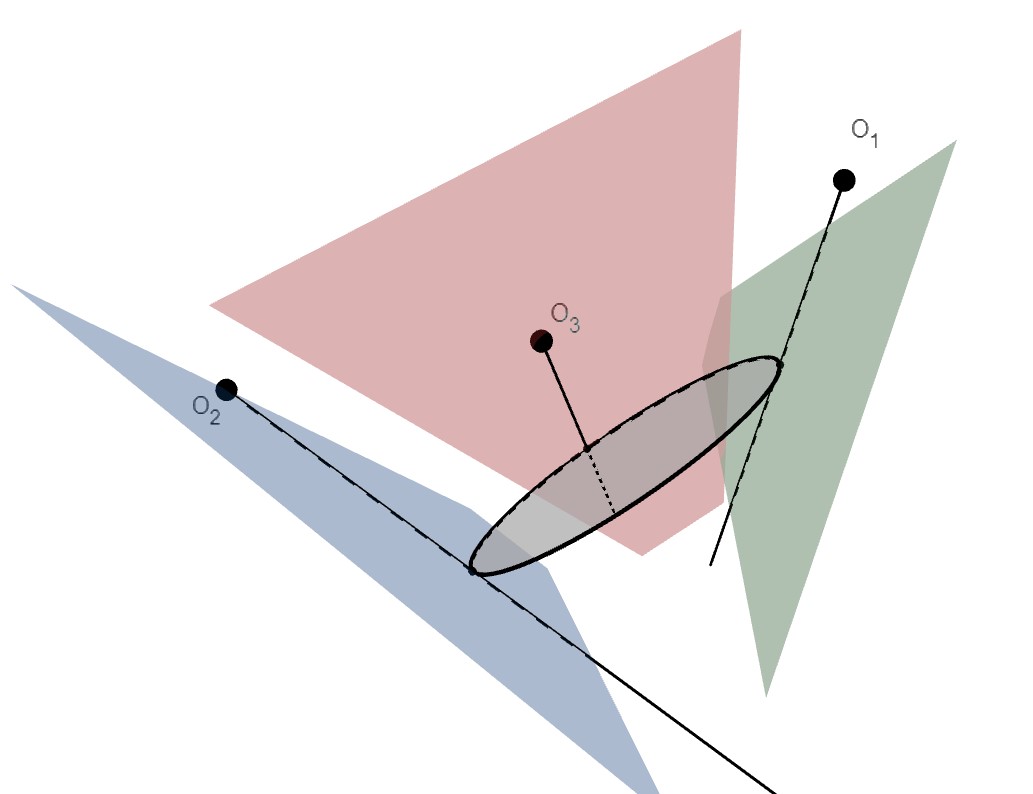
Each observed line $\boldsymbol{\ell}_{i}$ may be described in primal coordinates as the column span of the $4\times 2$ matrix

Here $\textbf{\emph{x}}_{i}\in{\mathbb{R}}^{3}$ gives the coordinates of the observer point $O_{i}$ and $\textbf{\emph{u}}_{i}\in\mathcal{S}^{2}$ a point on the unit sphere, representing a line-of-sight measurement. The bearings, in noiseless scenarios, are unit vectors pointing from observers towards points on the orbit.

Dually, $\boldsymbol{\ell}_{i}$ may be represented by any full-rank $4\times 2$ matrix $\textbf{\emph{A}}_{i}$ such that

Many choices are possible for the matrix $\textbf{\emph{A}}_{i}$ giving the dual representation of $\boldsymbol{\ell}_{i}$. In the next subsection, we explain two methods—one algebraic, and the other numerical—by which a suitable $\textbf{\emph{A}}_{i}$ may be directly computed from observations. Once $\textbf{\emph{A}}_{i}$ is computed, the tangent plane $\boldsymbol{\pi}_{i}$ may be written as

for a $2\times 1$ vector $\textbf{\emph{c}}_{i}.$ Substituting this expression into Eq. (16) yields

The nonzero vector $\textbf{\emph{c}}_{i}$, which depends on the unknown tangent plane, may be eliminated from this equation to obtain a constraint depending only on the observed line and the unknown entries of the disk quadric. Specifically,

Thus, each of the observed lines $\boldsymbol{\ell}_{1},\ldots,\boldsymbol{\ell}_{n}$ places a constraint on the 3D conic that is polynomial in the entries of $\textbf{\emph{A}}_{i}$ and $\textbf{\emph{Q}}^{*}.$ These are the basic constraints from which we may determine the unknown orbit.

Once we have obtained the disk quadric $\textbf{\emph{Q}}^{*}$, recovering the classical orbital elements is straightforward. This is essentially the reverse mapping to the relationship described by Eq. (12). Given the disk quadric $\textbf{\emph{Q}}^{*}$, we can directly compute the ellipse semi-minor axis $b$ as

and the focal distance $c$ as

Consequently, the semi-major axis and the eccentricity exploiting the relations $a=b^{2}+c^{2}$ and $e=c/a$. Then, we can find p as

and we can write

Using the fact that q is a unit vector, we finally obtain for some $i=1,2,3$ that

Here $i$ may be chosen such that the selected column of $\textbf{\emph{q}}\textbf{\emph{q}}^{T}$ has largest norm, so as to avoid numerical issues.

Determining $i$, $\Omega$ and $\omega$ from p and q can be done using standard relations that can be found, for example, in Vallado.

Determining the true anomaly corresponding to a bearing measurement requires a few more steps. Let $\textbf{\emph{x}}_{0}$ and $\textbf{\emph{u}}_{0}$ be the observer’s position and the observed direction relative to that bearing. The coordinates of the observed point along the orbit are given by

for some $\lambda\in\mathbb{R}$. The corresponding coordinates in $\mathbb{P}^{3}$ are:

Since the satellite’s position must be a point of the orbital plane $\boldsymbol{\beta}$, with

the following relationship allows us to determine $\lambda$

which gives

Substituting this expression for $\lambda$ inside Eq. (38), we can finally solve for the true anomaly corresponding to the bearing as the angle between the periapsis direction, enclosed in g (or p), and the position vector $\textbf{\emph{r}}_{0}$:

Note that $\lambda$ is also the range between the observer’s position and the satellite’s observed position. If desired, it is possible to correct for the light time-of-flight using $\lambda$, together with the time of a single measurement.

If we take a scaling factor of $1$ in the parameterization of $\textbf{\emph{Q}}^{*}$ given in Eq. (14), the seven unknown orbital parameters $\textbf{\emph{w}},\textbf{\emph{g}},b$ will be solutions to a system of $2+n$ equations given by Eqs. (15) and (21) for $i=1,\ldots,n.$ For sufficiently generic observations, we expect that when $7=2+n,$ or $n=5,$ this system of equations will have finitely many solutions. In fact, we expect the number of solutions to be constant if we count over the complex numbers. Such a “number conservation” principle may be viewed as a generalization of the fundamental theorem of algebra, which treats the case of a single polynomial in a single unknown. A formal statement in the language of algebraic geometry may be found, for instance, in Ref. (ShafarevichVol1, Theorem 2.29).

In the preceding paragraph, the precise meaning of the phrase “sufficiently generic” is that the vector of all observations $\begin{bmatrix}\textbf{\emph{x}}_{1}^{T}&\cdots&\textbf{\emph{x}}_{5}^{T}\,&\,\textbf{\emph{u}}_{1}^{T}&\cdots&\textbf{\emph{u}}_{5}^{T}\end{bmatrix}\in{\mathbb{R}}^{30}$ lies outside of an appropriately-defined discriminant locus. This discriminant locus is analogous to the commonly-known discriminant of a quadratic equation, but very difficult to describe explicitly (e.g., see (SturmfelsCBMS, Sec. 3.1) for an example with two unknowns.)

To see an example which is not sufficiently generic, we may consider any $5$ observations from any perfectly-circular orbit. In this case, the true orbit satisfies $\textbf{\emph{g}}=0$ and the corresponding solution is singular; that is, the $7\times 7$ Jacobian matrix of the system evaluated at this solution is rank-deficient. Such a singular solution may be difficult to estimate accurately with standard numerical methods. The same is true for the nearly-singular solutions arising from the practical case of nearly-circular orbits.

On the other hand, if we enforce the constraint of a circular orbit by requiring that $\textbf{\emph{g}}=0$, then $n=3$ observations suffice to recover the orbit up to finitely many possibilities. Under this circular model, we obtain another system of polynomial equations, from which we may compute the remaining orbital parameters $\textbf{\emph{w}},b$. Such a model has the advantage of needing fewer observations, and may potentially give a reasonable approximation of the true orbit in the nearly-circular case.

We summarize the two different orbit models, the associated polynomial systems, and how many solutions they have for generic data in Proposition 1.

The claims appearing in Proposition 1 regarding the number of solutions may be readily verified using any one of the standard methods for solving polynomial systems, such as Gröbner bases (see (CLO15, Ch. 2) for an overview), or polynomial homotopy continuation Sommese:2005. In our experiments, we solve the systems associated to either model using an implementation of the latter method provided by the software package NAG4M2 Ley11 in the computer algebra system Macaulay2 M2. We give an overview of homotopy continuation in the next subsection.

Numerical homotopy continuation is a general method which can be used to solve polynomial systems, such as those appearing in Proposition 1. The essential idea underlying the method is as follows: since the roots of polynomials vary continuously with their coefficients, we can use a system whose solution set is known (the start system) to solve some other system in the same class of systems (the target system) by estimating how the solutions change (path-tracking) as we deform one system into another. We use a short example to illustrate the main ideas.

The choice of the start system is an important factor when implementing any homotopy continuation method. Usually, we want a start system that is general enough to solve any possible target system coming from a specific application. Another important factor when choosing a start system is its specificity, or the number of start solutions. Different choices of start systems are compared in Ref. (Sommese:2005, Ch. 8), where a basic tradeoff is identified: a start system that is easy to describe and solves a large class of systems will typically require tracking more paths. For example, if the total-degree start system is used to solve an instance of the elliptical model, this requires tracking $4^{5}\times 2^{2}=4096$ paths. This should be compared with the optimal number of $66$ established by Proposition 1. If the total degree homotopy was to be used to solve the elliptical model, then we would need to track $4096-66=4030$ divergent solution paths with $\textbf{\emph{X}}(t)\to\infty$ as $t\to 1^{-}.$

In contrast to the total degree homotopy, parameter homotopies MR977815 allow us to track, under reasonable assumptions, the optimal number of paths. Since “most” instances of the systems in Proposition 1 will have the same number of solutions, any randomly-chosen instance may, in principle, be chosen as a start system. Parameter homotopies may be used in a general setting where we have a system $\textbf{\emph{F}}(\textbf{\emph{X}};\textbf{\emph{P}})=0$, with as many equations as unknowns, which depends polynomially both on the unknowns X and certain parameters P depending on the observations. For the systems of interest to us, there is some flexibility in how these parameters are chosen. One simple choice is that the target parameters $\textbf{\emph{P}}_{1}\in{\mathbb{R}}^{8n}$ consist of all dual coordinates of all $n$ lines—that is, $\textbf{\emph{P}}_{1}\in{\mathbb{R}}^{40}$ for the elliptical model, and $\textbf{\emph{P}}_{0}\in{\mathbb{R}}^{24}$ for the circular model. Alternatively, using Eq. (25), we may directly encode the observer and bearing vectors into a parameter vector $\textbf{\emph{P}}_{1}\in{\mathbb{R}}^{6n}$—that is, $\textbf{\emph{P}}_{1}\in{\mathbb{R}}^{30}$ for the elliptical model, and $\textbf{\emph{P}}_{1}\in{\mathbb{R}}^{18}$ for the circular model. The following description of parameter homotopies applies equally well to either choice.

In general, the parameter values $\textbf{\emph{P}}_{1}$ encoded by a set of observations specify the target system $\textbf{\emph{F}}(\textbf{\emph{X}};\textbf{\emph{P}}_{1})=0$ of the parameter homotopy. If there are $m$ parameter values, i.e., $\textbf{\emph{P}}_{1}\in{\mathbb{R}}^{m}$, then the start system should also be a $m\times 1$ vector $\textbf{\emph{P}}_{0}.$ For the start system $\textbf{\emph{F}}(\textbf{\emph{X}};\textbf{\emph{P}}_{0})=0,$ we are given a pre-computed set of $d\in\{12,66\}$ complex solutions $\textbf{\emph{X}}_{1}(0),\ldots,\textbf{\emph{X}}_{d}(0)$ whose coordinates are the unknown orbital elements which are pairwise-inequivalent up to the sign-symmetries described in Proposition 1. To extend these start solutions to solution paths $\textbf{\emph{X}}_{1}(t),\ldots,\textbf{\emph{X}}_{d}(t),$ we “deform” the start system into the target system via the parameter homotopy

Each solution path $\textbf{\emph{X}}(t)$ is an implicit function of $t$ satisfying Eq. (45) and the nonlinear ODE system

This ODE, together with one of the start solutions $\textbf{\emph{X}}_{i}(0)$, gives an initial value problem for an unknown solution path $\textbf{\emph{X}}_{i}(t)$ satisfying Eq. (45). Numerical integration methods allow us to estimate $\textbf{\emph{X}}_{i}(t)$ for $t\in[0,1].$ In practice, we approximate a solution path using numerical/predictor corrector methods. If $\textbf{\emph{X}}_{i}(t)$ is known within some tolerance for some $t\in[0,1],$ then a “predictor step” (typically the standard fourth-order Runge-Kutta method) uses Eq. (46) to find an initial estimate for $\textbf{\emph{X}}_{i}(t+\Delta t)$ for some step-size $\Delta t.$ This estimate is subsequently refined by a “corrector step” using one or more iterations of Newton’s method.

A key property of parameter homotopies is that, under mild hypotheses, they are globally convergent with probability-one. The following key properties of the parameter homotopy in Eq. (45) are consequences of a more general parameter continuation theorem (Sommese:2005, Theorem 7.1.1). We specialize this general result to our case of particular interest. For sufficiently generic (and hence, almost all) $(\textbf{\emph{P}}_{0},\textbf{\emph{P}}_{1}),$ we have:

1. 1.

   Each start solution $\textbf{\emph{X}}_{i}(0)$ extends to a solution path $\textbf{\emph{X}}_{i}(t)$ which is smooth for all $t\in[0,1].$

2. 2.

   Every solution to the target system may be obtained up to sign-symmetry from the endpoint $\textbf{\emph{X}}_{i}(1)$ of some solution path $\textbf{\emph{X}}_{i}(t).$

At this point, it is worth pointing out key differences between homotopy continuation, a global root-finding method, from a more standard local approach like Newton’s method. In Newton’s method, we would pick a single “start solution” X, then compute iterates $\textbf{\emph{X}}\leftarrow\textbf{\emph{X}}-\textbf{\emph{F}}(\textbf{\emph{X}};\textbf{\emph{P}}_{1})$ until some convergence condition is satisfied, yielding a single solution to the target system $\textbf{\emph{F}}(\textbf{\emph{X}};\textbf{\emph{P}}_{1})=0.$ In practice, this may suffer if the initial guess for X is not sufficiently close to a target solution.

In homotopy continuation, “start solutions” instead refer to solutions to the start system $\textbf{\emph{F}}(\textbf{\emph{X}};\textbf{\emph{P}}_{0})=0$ which have been pre-computed. There is no requirement that these start solutions be “close” to solutions of the target system, nor that the start and target parameters be close in the space of all parameters. As long as the pre-computed start parameters $\textbf{\emph{P}}_{0}\in{\mathbb{C}}^{m}$ are sufficiently generic, all start solutions can be numerically continued from $t=0$ to $t=1.$ Thus, we can compute all solutions to the target system $\textbf{\emph{F}}(\textbf{\emph{X}};\textbf{\emph{P}}_{1})=0,$ provided that the target parameters $\textbf{\emph{P}}_{1}$ are also sufficiently generic.

Usually, choosing random complex numbers for the start parameters $\textbf{\emph{P}}_{0}$ will be sufficient to ensure that all isolated solutions of the target system specified by $\textbf{\emph{P}}_{1}$ can be computed. As such, the choice of start parameters, provided that they are sufficiently random, may be expected to have relatively little impact on the accuracy of the computed target solutions. Here, “accuracy” describes the distance between a true target solution and the approximation that is computed by homotopy continuation. In the absence of measurement noise, the truth is usually recovered to within machine precision. With measurement noise, the accuracy is dependent on the amount of noise (i.e., more noise results in poorer accuracy). Regardless of the presence (or magnitude) of noise, there is no clear, simple criterion for picking a “good” start system that may lead to more accurate results. However, there are some properties of the start parameters that we can aim to optimize. For instance, if the Jacobian matrices $\displaystyle\frac{d\textbf{\emph{H}}}{d\textbf{\emph{X}}}(\textbf{\emph{X}}_{i}(0);\textbf{\emph{P}}_{0})$ are well-conditioned for each of the start solutions $\textbf{\emph{X}}_{i}(0)$, then for each solution path we can expect the predictor/corrector steps to be more accurate when $t$ is near $0.$ With this in mind, our choice of start system was based on generating several different sets of parameters $\textbf{\emph{P}}_{0}$ at random, with coordinates drawn uniformly from the complex unit circle, computing a complete set of solutions for each system, and selecting the system whose maximum condition number over all solutions was smallest. To solve the parametric systems in each model for an initial set of parameters, we used an approach based on monodromy, which works well in tandem with parameter homotopies and can naturally exploit the four-fold symmetry in solutions. We refer to Refs. MR3984062; https://doi.org/10.48550/arxiv.2105.04460; https://doi.org/10.48550/arxiv.1612.08807 for more details about this approach.

In our implementation, we use Eq. (27) to determine the parameters representing the dual coordinates of each line-of-sight observation. Before solving, we rescale all distance measurements into units of earth-radii, which has the typical effect of making the entries of $\textbf{\emph{Q}}^{*}$ comparable in magnitude. We use the default path-tracker settings in NAG4M2, except that a minimum stepsize of $\Delta t=$1\text{\times}{10}^{-16}$$ is used. Additionally, we handle (infrequent) cases of path failure for $t\approx 1$ using Cauchy’s endgame for estimating singular solutions (Sommese:2005, Ch. 10).

For $n>5$ observations, an exact solution satisfying all $n+2$ constraints of Eqs. (21) and (15) typically will not exist. However, we can still aim to minimize some cost function $J$ that depends on all $n$ measurements. One simple choice based on Eq. (21) is a sum of squared equation residuals,

Our task is now to minimize $J(\textbf{\emph{Q}}^{*})$ while enforcing the constraints from Eq. (15). To solve this constrained optimization problem, we use the method of Lagrange multipliers to compute all complex-valued critical points. For $n>5$ generic observations, the number of critical points turns out to be $4244=4\times\textbf{1061}$ critical points. A solution of minimum cost among the physically-plausible critical points then provides an estimate for the unknown orbit.

To obtain polynomial equations from Eqs. (47) and (15), we may set $\beta=-1/b^{2}$ and write down the (homogenized) Lagrangian function,

The first-order optimality conditions then read

Imposing a generic affine-linear equation

we obtain a system of 10 equations (from Eqs. (49) and (50)) in 10 unknowns, depending on the observations $\textbf{\emph{A}}_{1},\ldots,\textbf{\emph{A}}_{n}$ and the new parameters $c_{0},\ldots,c_{3}.$ As before, the solutions obey a 4-fold symmetry, and we may track 1061 paths using parameter homotopies to compute all solutions for generic parameter values. With this general setup, one may make the usual choice of parameters $(c_{0},c_{1},c_{2},c_{3})=(1,0,0,-1)$ to obtain $\lambda_{0}=1$. However, to improve numerical stability (Bertinibook, Sec 4.7), we choose these four parameters in our experiments uniformly at random from the unit $3$-sphere in ${\mathbb{R}}^{4}$.

Since most orbits of interest are nearly circular, we chose a nearly-circular orbit as a first test case for the performance of this purely geometric method. Specifically, we took inspiration from the orbit traveled by the satellite of the AQUA mission Parkinson:2003. Its orbital elements can be found in Table 2.

We obtained simulated observer data considering observations gathered by different ground stations. Ten observers are given in geocentric coordinates, in units of Earth radii, by

A corresponding set of unit-length bearings is obtained from known points along the orbit:

The true orbit’s disk quadric $\textbf{\emph{Q}}^{*}$ is

Since the eccentricity of the orbit is $e=$$1.5\text{\times}{10}^{-3}$, we might expect that the circular model gives a reasonable approximation of the true orbit. Thus, to obtain a preliminary assessment of the feasibility of using parameter homotopies for this IOD scenario, we considered both the circular and elliptical models. In this experiment, $100$ random observer-bearing correspondences were sampled, from a total $120=\binom{10}{3}$ possibilities for the circular model and $252=\binom{10}{5}$ for the elliptical model, and the corresponding polynomial systems appearing in Proposition 1 were solved. Mean and standard deviation of the estimated disk quadric and of the orbital parameters for this experiment are reported in Table 3. For the circular model, we do not report the argument of periapsis $\omega$ since it is undefined.

The homotopy solvers for both models run on the order of less than a second. The average runtimes for the elliptical model and the circular model of 0.67 seconds and 0.13 seconds, respectively, differ by a factor of roughly $5$. This is due largely to the fact that there are $66/12=5.5$ times as many paths to track in the elliptical model vs the circular model. Additionally, we used a very conservative value of $1\text{\times}{10}^{-16}$ for the minimum value of the predictor/corrector stepsize $\Delta t$, so as to guard against potential failures when tracking solution paths.

Under the elliptical model, Table 3 shows that we can recover the true orbit to nearly machine precision in the absence of measurement noise. Errors under the circular model are uniformly higher due to model mismatch, but still small. We will show later in this section how the circular model may sometimes be preferable in particular situations.

To illustrate our proposed method of orbit determination on an example from the nearly-circular case, we now focus on a particular set of observers and bearings which appear in Fig. 5, corresponding to columns $1,4,5,6,9$ in the observer and bearing matrices above.

Note that one of the observations considered is nearly coplanar with the orbital plane, a condition that is singular for the solver, and that is expected to lower its accuracy in presence of noise. In the case of ideal observations, under the elliptical model, $44$ of the $66$ complex solutions recovered by the solver give a real-valued disk quadric. However, only $3$ of these real disk quadrics can be lifted to real-valued orbital parameters $(\textbf{\emph{w}},\textbf{\emph{g}},b)$ (see Rem. 1.) These real solutions are given, modulo the sign ambiguity, by

The solution $\textbf{\emph{X}}_{3}$ corresponds to the true orbit. To rule out the additional real solutions, a sixth line coming from the observation $(\textbf{\emph{x}}_{2},\textbf{\emph{u}}_{2})$ may be used. Evaluating the left-hand side of Eq. 21 for this line at both solutions $\textbf{\emph{X}}_{1}$ and $\textbf{\emph{X}}_{2}$ gives residual errors of $$3.9\text{\times}{10}^{-3}$,$4.6\text{\times}{10}^{-4}$,$ and $6.2\text{\times}{10}^{-16}$, respectively. Thus, the solution $\textbf{\emph{X}}_{3}$ gives the best fit to the sixth observation.

Applying the circular model to this same example (with observations 1, 5, and 6), there are now $6$ real solutions up to sign ambiguity in the nonzero parameters $(\textbf{\emph{w}},b).$ However, all $5$ original observations may now be used to remove the $5$ extraneous solutions. Evaluating the residuals of constraints 21 on these additional solutions as with the elliptical model allows us to distinguish the correct solution. Another comparison between the true orbit and the extraneous solutions may be obtained by computing the distance from each of the five estimated orbit points to the origin. For the three observations used in the homotopy solver these distances all equal $b,$ but these distances may be significantly different for the two unused observations. For each of the 6 real solutions, we may compute the variance of the set of three distances comprised of $b$ and the unused observations. One of these values is $1\text{\times}{10}^{-9}$, and the rest are on the order of $1\text{\times}{10}^{-3}$ or higher. This strongly signals the best approximation of the true solution, which is given by

As a second test case, we consider an orbit close to that traveled by the Magnetospheric Multiscale Spacecrafts (MMS) Fuselier:2014. This is a highly-elliptical orbit, whose orbital elements we report in Table 4.

In this scenario, 10 observations were obtained with three ground stations on the Earth’s surface, and we evaluated the runtime and accuracy on 100 sets of five noiseless observations. The summary statistics shown in Table 5 demonstrate that the solver for the elliptical model is efficient and highly accurate in all cases. Its average runtime was of 0.56 seconds. Note that we do not consider the circular model.

References

- (1) Gauss, C.F.: Theoria Motus Corporum Coelestium in Sectionibus Conicis Solem Ambientum. F. Perthes and I.H. Besser, Hamburg (1809)
- (2) Laplace, S.: Mémoire sur la détermination des orbites des comètes. Mémoires de Mathématique et de Physique, 13–72 (1780)
- (3) Gibbs, J.: On the determination of elliptic orbits from three complete observations. Memoirs of the National Academy of Sciences 4(8), 79–104 (1889)
- (4) Hollenberg, C.L., Christian, J.A.: Geometric solutions for problems in velocity-based orbit determination. Journal of the Astronautical Sciences 67, 188–224 (2019). https://doi.org/10.1007/s40295-019-00170-7
- (5) Gooding, R.H.: A new procedure for the solution of the classical problem of minimal orbit determination from three lines of sight. Celestial Mechanics and Dynamical Astronomy 66, 387–423 (1997)
- (6) Escobal, P.R.: Methods of Orbit Determination, 2nd edn. Robert E. Krieger Publishing Company, Malabar, FL (1976)
- (7) Lambert, I.H.: Insigniores Orbitae Cometarum Proprietates (1761). Kessinger’s Legacy Reprints. Kessinger Publishing, Whitefish, MT (2010)
- (8) Christian, J.A.: Initial orbit determination from only heading measurements. Journal of Spacecraft and Rockets (2023). https://doi.org/10.2514/1.A35593
- (9) Semple, J.G., Kneebone, G.T.: Algebraic Projective Geometry, pp. 47–48. Oxford University Press, Oxford, UK (1952)
- (10) Hartley, R., Zisserman, A.: Multiple View Geometry, 2nd Ed. Cambridge University Press, Cambridge, UK (2003)
- (11) Christian, J.A.: A tutorial on horizon-based optical navigation and attitude determination with space imaging systems. IEEE Access, 19819–19853 (2021). https://doi.org/10.1109/ACCESS.2021.3051914
- (12) Christian, J.A., Derksen, H., Watkins, R.: Lunar crater identification in digital images. The Journal of the Astronautical Sciences 68, 1056–1144 (2021). https://doi.org/10.1007/s40295-021-00287-8
- (13) Christian, J.A.: Analytic initial orbit determination using satellite streaks in digital image. In: AAS/AIAA Astrodynamics Specialist Conference (2021)
- (14) Henry, S., Christian, J.A.: Absolute triangulation algorithms for space exploration. Journal of Guidance, Control, and Dynamics 46(1), 21–46 (2023). https://doi.org/10.2514/1.G006989
- (15) Mancini, M.: An analysis on the application of algebraic geometry in initial orbit determination problems. Master’s thesis, Georgia Institute of Technology (2022)
- (16) Vallado, D.A.: Fundamentals of Astrodynamics and Applications, (2013)
- (17) Shafarevich, I.R.: Basic Algebraic Geometry. 1, 2nd edn., p. 303. Springer, Berlin (1994). Varieties in projective space, Translated from the 1988 Russian edition and with notes by Miles Reid
- (18) Sturmfels, B.: Solving Systems of Polynomial Equations. CBMS Regional Conference Series in Mathematics, vol. 97. Published for the Conference Board of the Mathematical Sciences, Washington, DC; by the American Mathematical Society, Providence, RI
- (19) Cox, D.A., Little, J., O’Shea, D.: Ideals, Varieties, and Algorithms: An Introduction to Computational Algebraic Geometry and Commutative Algebra, 4th edn. Undergraduate Texts in Mathematics, p. 646. Springer, Cham (2015). https://doi.org/10.1007/978-3-319-16721-3
- (20) Sommese, A., Wampler, C.: The Numerical Solution of Systems of Polynomial Arising in Engineering and Science vol. 2005, (2005). https://doi.org/10.1142/9789812567727
- (21) Leykin, A.: Numerical algebraic geometry. J. Softw. Algebra Geom. 3, 5–10 (2011). https://doi.org/10.2140/jsag.2011.3.5
- (22) Grayson, D.R., Stillman, M.E.: Macaulay2, a software system for research in algebraic geometry. Available at http://www.math.uiuc.edu/Macaulay2/
- (23) Morgan, A.P., Sommese, A.J.: Coefficient-parameter polynomial continuation. Appl. Math. Comput. 29(2, part II), 123–160 (1989). https://doi.org/10.1016/0096-3003(89)90099-4
- (24) Duff, T., Hill, C., Jensen, A., Lee, K., Leykin, A., Sommars, J.: Solving polynomial systems via homotopy continuation and monodromy. IMA J. Numer. Anal. 39(3), 1421–1446 (2019). https://doi.org/10.1093/imanum/dry017
- (25) Duff, T., Korotynskiy, V., Pajdla, T., Regan, M.H.: Galois/monodromy groups for decomposing minimal problems in 3D reconstruction. arXiv (2021). https://doi.org/10.48550/ARXIV.2105.04460. https://arxiv.org/abs/2105.04460
- (26) Améndola, C., Lindberg, J., Rodriguez, J.I.: Solving Parameterized Polynomial Systems with Decomposable Projections. arXiv (2016). https://doi.org/10.48550/ARXIV.1612.08807. https://arxiv.org/abs/1612.08807
- (27) Bates, D.J., Hauenstein, J.D., Sommese, A.J., Wampler, C.W.: Numerically Solving Polynomial Systems with Bertini. Software, Environments, and Tools, vol. 25, p. 352. Society for Industrial and Applied Mathematics (SIAM), Philadelphia, PA (2013)
- (28) Parkinson, C.L.: Aqua: An earth-observing satellite mission to examine water and other climate variables. IEEE Transactions on Geoscience and Remote Sensing 41(2), 173–183 (2003)
- (29) Fuselier, S.A., Lewis, W.S., Schiff, C., Ergun, R., Burch, J.L., Petrinec, S.M., Trattner, K.J.: Magnetospheric multiscale science mission profile and operations. Space Science Reviews, 77–103 (2014). https://doi.org/10.1007/s11214-014-0087-x
- (30) Shuster, M.D., Oh, S.D.: Three-axis attitude determination from vector observations. Journal of Guidance and Control 4(1), 70–77 (1981). https://doi.org/10.2514/3.19717
- (31) Shuster, M.D.: Maximum likelihood estimation of spacecraft attitude. The Journal of the Astronautical Sciences 37(1), 79–88 (1989)
- (32) Baker, R.M.L., Jacoby, N.H.: Preliminary orbit-determination method having no co-planar singularity”. Celestial Mechanics 15, 137–160 (1977). https://doi.org/10.1007/BF01228460
- (33) Bannister, M., et al.: The natural history of ‘Oumuamua. Nature Astronomy 3(7), 594–602 (2019). https://doi.org/10.1038/s41550-019-0816-x