跳到论文正文
W Papers独立论文阅读器 arXiv:2304.02062 论文正文 计算阅读时间 · 0%
引用这篇论文根据当前论文元数据生成,正式投稿前建议核对。


License: arXiv.org perpetual non-exclusive license
arXiv:2304.02062v4 [math.NA] 09 Apr 2026
\setbibdata

0000002025 An Error Estimator for Electrically Coupled LCs

An A Posteriori Error Estimator for Electrically Coupled Liquid Crystal Equilibrium Configurations

J.H. Adler22 2 Tufts University, Medford MA 02155, USA (james.adler@tufts.edu)    D.B. Emerson33 3 Vector Institute, Toronto ON M5G 1M1, Canada (david.emerson@vectorinstitute.ai)
Abstract

This paper derives an a posteriori error estimator for the nonlinear first-order optimality conditions associated with the electrically and flexoelectrically coupled Frank-Oseen model of liquid crystals, building on previous results for elastic systems. The estimator is proposed for a penalty approach to imposing the unit-length constraint required by the model. Moreover, theory is proven establishing that the estimator provides a reliable estimate of global approximation error and an efficient measure of local error, suitable for use in adaptive refinement. Numerical experiments demonstrate significant improvements in efficiency with adaptive refinement guided by the proposed estimator in a multilevel, nested-iteration framework and superior physical properties for challenging electrically coupled systems.

keywords
liquid crystal simulation, coupled systems, a posteriori error estimators, adaptive mesh refinement
{AMS}

76A15, 65N30, 49M15, 65N22, 65N55

1 Introduction

As materials possessing mesophases with characteristics of both liquids and organized solids, liquid crystals exhibit many interesting physical properties inspiring extensive study and a wide range of applications. In addition to considerable use in modern display technologies, liquid crystals are used for nanoparticle organization [17], manufacture of structured nanoporous solids [29], and efficient conversion of mechanical strain to electrical energy [15], among many others.

The focus of this paper is nematic liquid crystals, which are rod-like molecules with long-range orientational order described by a vector field 𝐧⁡(x,y,z)=(n1,n2,n3)T{\bf{n}}(x,y,z)=(n_{1},n_{2},n_{3})^{T}, referred to as the director. For the model considered here, 𝐧{\bf{n}} is constrained to unit-length pointwise throughout the domain, Ω\Omega. In addition to their elastic properties, liquid crystals are dielectrically active such that their structures are affected by the presence of electric fields. In addition, certain types of liquid crystals demonstrate flexoelectric coupling wherein deformations of the director produce internally generated electric fields [19]. Thorough treatments of liquid crystal physics are found in [24, 28].

With the combination of highly-coupled physics and complicated experimental behavior, numerical simulations of liquid crystal structures are fundamental to the study of novel physical phenomena, optimization of device design, and analysis of experimental observations [13, 9, 22]. As many applications and experiments require simulations on two- and three-dimensional domains with complicated boundary conditions, the development of highly efficient and accurate numerical approaches is important. Effective a posteriori error estimators significantly increase the efficiency of numerical methods for partial differential equations (PDEs) and variational systems by guiding the construction of optimal discretizations via adaptive refinement. A wealth of research exists for the design and theoretical support of effective error estimators in the context of finite-element methods. This includes techniques treating both linear and nonlinear PDEs across a number of applications (see, e.g., [16, 20, 25, 6, 4]).

In [12], a reliable a posterior error estimator was developed for the first-order optimality conditions arising from minimization of the Frank-Oseen elastic free-energy model. Using the estimator to guide adaptive mesh refinement (AMR) in numerical simulations, produced competitive solutions in terms of constraint conformance and free energy with considerably less computational work. In this paper, the elastic error estimator is extended to consider systems with electric and flexoelectric coupling. The proposed, coupled, a posteriori error estimator is shown to be a reliable estimate of global approximation error and an efficient indicator of local error. The incorporation of electric and flexoelectric fields produce a markedly more complicated estimator and auxiliary spaces requiring careful theoretical treatment. In certain cases, modifications of the original theory in [12] are straightforward. In others, however, important adjustments must be made to ensure that the framework of [26, 27] remains viable. Numerical experiments leveraging a multilevel nested-iteration framework for problems with both external and flexoelectrically induced electric fields demonstrate the performance of the estimator compared with uniform refinement.

This paper is organized as follows. In Section 2, the coupled Frank-Oseen free-energy model and associated variational system for the first-order optimality conditions is introduced. Additional notation and prerequisite theoretical results to be applied in the reliability and efficiency proofs are discussed in Section 3. In Section 4, the specific coupled error estimator is derived and proofs of reliability and efficiency are constructed. Section 5 presents numerical experiments demonstrating the performance of the error estimator and a multilevel AMR approach. Finally, Section 6 provides some concluding remarks and a discussion of future work.

2 Free-Energy Model and Optimality Conditions

Liquid crystals are simulated using a number of different models [10, 21, 14]. Here, the Frank-Oseen free-energy model is considered where, for a domain Ω\Omega, the coupled equilibrium free energy is composed of three main components associated with elastic deformations, external electric fields, and flexoelectrically generated fields. The coupled free-energy functional is then written

(1) 𝒢⁡(𝐧,ϕ)\displaystyle\mathcal{G}({\bf{n}},\phi) =12K1∥∇⋅𝐧∥02+12K3⟨𝐙∇×𝐧,∇×𝐧⟩0−12ϵ0ϵ⟂⟨∇ϕ,∇ϕ⟩0\displaystyle=\frac{1}{2}K_{1}\|{\bf{\nabla}}\cdot{\bf{n}}\|_{0}^{2}+\frac{1}{2}K_{3}\langle{\bf{Z}}{\bf{\nabla}}\times{\bf{n}},{\bf{\nabla}}\times{\bf{n}}\rangle_{0}-\frac{1}{2}\epsilon_{0}\epsilon_{\perp}\langle\nabla\phi,\nabla\phi\rangle_{0}
−12ϵ0ϵa⟨𝐧⋅∇ϕ,𝐧⋅∇ϕ⟩0+es⟨∇⋅𝐧,𝐧⋅∇ϕ⟩0+eb⟨𝐧×∇×𝐧,∇ϕ⟩0,\displaystyle\hskip 9.95863pt-\frac{1}{2}\epsilon_{0}\epsilon_{a}\langle{\bf{n}}\cdot\nabla\phi,{\bf{n}}\cdot\nabla\phi\rangle_{0}+e_{s}\langle{\bf{\nabla}}\cdot{\bf{n}},{\bf{n}}\cdot\nabla\phi\rangle_{0}+e_{b}\langle{\bf{n}}\times{\bf{\nabla}}\times{\bf{n}},\nabla\phi\rangle_{0},

where we denote the classical L2​(Ω)L^{2}(\Omega) inner product and norm as ⟨⋅,⋅⟩0\langle\cdot,\cdot\rangle_{0} and ∥⋅∥0\|\cdot\|_{0}, respectively, for both scalar and vector quantities. The variable ϕ\phi in (1) denotes the electric potential for an electric field, 𝐄{\bf{E}}, such that 𝐄=∇ϕ{\bf{E}}=\nabla\phi. Here, Ki≥0K_{i}\geq 0, i=1,2,3i=1,2,3 are the Frank constants, which depend on the physical characteristics of the liquid crystal and have a significant impact on orientational structure [3, 18]. Assuming that each Ki≠0K_{i}\neq 0, we define the tensor 𝐙=𝐈−(1−κ)​𝐧⊗𝐧{\bf{Z}}={\bf{I}}-(1-\kappa){\bf{n}}\otimes{\bf{n}}, where κ=K2/K3\kappa=K_{2}/K_{3}. The permittivity of free space is denoted by ϵ0>0\epsilon_{0}>0. The dielectric anisotropy of the liquid crystal is ϵa=ϵ∥−ϵ⟂\epsilon_{a}=\epsilon_{\parallel}-\epsilon_{\perp}, with the constants ϵ∥,ϵ⟂>0\epsilon_{\parallel},\epsilon_{\perp}>0 representing the parallel and perpendicular dielectric permittivity, respectively. For positive ϵa\epsilon_{a}, the director favors parallel alignment with the electric field, while negative anisotropy indicates a perpendicular preference. Finally, ese_{s} and ebe_{b} are material constants specifying the liquid crystal’s flexoelectric response.

Equilibrium states correspond to configurations that minimize the functional in (1) subject to the local unit-length constraint, 𝐧⋅𝐧−1=0{\bf{n}}\cdot{\bf{n}}-1=0, on Ω\Omega. Additionally, the relevant Maxwell’s equations for a static electric field, ∇⋅𝐃=0{\bf{\nabla}}\cdot{\bf{D}}=0 and ∇×𝐄=𝟎{\bf{\nabla}}\times{\bf{E}}={\bf{0}}, known as Gauss’ and Faraday’s laws, respectively, must be satisfied. For this system,

𝐃=−ϵ0ϵ⟂∇ϕ−ϵ0ϵa(𝐧⋅∇ϕ)𝐧+es𝐧(∇⋅𝐧)+eb(𝐧×∇×𝐧).\displaystyle{\bf{D}}=-\epsilon_{0}\epsilon_{\perp}\nabla\phi-\epsilon_{0}\epsilon_{a}({\bf{n}}\cdot\nabla\phi){\bf{n}}+e_{s}{\bf{n}}({\bf{\nabla}}\cdot{\bf{n}})+e_{b}({\bf{n}}\times{\bf{\nabla}}\times{\bf{n}}).

Note that the use of an electric potential implies that Faraday’s law is trivially satisfied, and it is straightforward to show that a minimizing pair, (𝐧∗,ϕ∗)({\bf{n}}_{*},\phi_{*}), adhering to the unit-length constraint, satisfies Gauss’ law in weak form. For a full derivation of the functional in (1), see [1, 13]. Throughout this paper, the presence of Dirichlet boundary conditions is assumed. Therefore the functional has been simplified using the null Lagrangian discussed in [24]. Moreover, the free-energy expression has been non-dimensionalized using the approach detailed in [2].

Throughout this paper, it is assumed that 𝐧∈(H𝐠11​(Ω))3={𝐯∈(H1​(Ω))3:𝐯=𝐠1​ on ​∂Ω}{\bf{n}}\in\left(H_{{\bf{g}}_{1}}^{1}(\Omega)\right)^{3}=\{{\bf{v}}\in\left(H^{1}(\Omega)\right)^{3}:{\bf{v}}={\bf{g}}_{1}\text{ on }\partial\Omega\} and ϕ∈Hg21​(Ω)={ψ∈H1​(Ω):ψ=g2​ on ​∂Ω}\phi\in H_{g_{2}}^{1}(\Omega)=\{\psi\in H^{1}(\Omega):\psi=g_{2}\text{ on }\partial\Omega\}, where H1​(Ω)H^{1}(\Omega) denotes the standard Sobolev space with norm ∥⋅∥1\|\cdot\|_{1}. The boundary functions 𝐠1{\bf{g}}_{1} and g2g_{2} are assumed to satisfy appropriate compatibility conditions for the domain. Note that if 𝐠1=𝟎{\bf{g}}_{1}={\bf{0}}, the space (H𝐠11​(Ω))3=(H01​(Ω))3\left(H^{1}_{{\bf{g}}_{1}}(\Omega)\right)^{3}=\left(H^{1}_{0}(\Omega)\right)^{3}.

The penalty approach studied in [1, 2] is used to enforce the pointwise unit-length constraint. The penalty method adds a weighted, positive term to the free-energy functional, penalizing deviation from the constraint such that for ζ>0\zeta>0

ℋ⁡(𝐧,ϕ)=𝒢⁡(𝐧,ϕ)+12​ζ​⟨𝐧⋅𝐧−1,𝐧⋅𝐧−1⟩0.\displaystyle\mathcal{H}({\bf{n}},\phi)=\mathcal{G}({\bf{n}},\phi)+\frac{1}{2}\zeta\langle{\bf{n}}\cdot{\bf{n}}-1,{\bf{n}}\cdot{\bf{n}}-1\rangle_{0}.

Taking the first variation of ℋ⁡(𝐧,ϕ)\mathcal{H}({\bf{n}},\phi), the first-order optimality conditions are written

(2) 𝒫⁡(𝐧,ϕ)=𝒞⁡(𝐧,ϕ)+2​ζ​⟨𝐯⋅𝐧,𝐧⋅𝐧−1⟩0=0\displaystyle\mathcal{P}({\bf{n}},\phi)=\mathcal{C}({\bf{n}},\phi)+2\zeta\langle{\bf{v}}\cdot{\bf{n}},{\bf{n}}\cdot{\bf{n}}-1\rangle_{0}=0 ∀(𝐯,ψ)∈H01​(Ω)3×H01​(Ω),\displaystyle\forall({\bf{v}},\psi)\in H^{1}_{0}(\Omega)^{3}\times H^{1}_{0}(\Omega),

where

𝒞(𝐧,ϕ)=K1⟨∇⋅𝐧,∇⋅𝐯⟩0+K3⟨𝐙∇×𝐧,∇×𝐯⟩0−ϵ0ϵa⟨𝐧⋅∇ϕ,𝐯⋅∇ϕ⟩0\displaystyle\mathcal{C}({\bf{n}},\phi)=K_{1}\langle{\bf{\nabla}}\cdot{\bf{n}},{\bf{\nabla}}\cdot{\bf{v}}\rangle_{0}+K_{3}\langle{\bf{Z}}{\bf{\nabla}}\times{\bf{n}},{\bf{\nabla}}\times{\bf{v}}\rangle_{0}-\epsilon_{0}\epsilon_{a}\langle{\bf{n}}\cdot\nabla\phi,{\bf{v}}\cdot\nabla\phi\rangle_{0}
+(K2−K3)⟨𝐧⋅∇×𝐧,𝐯⋅∇×𝐧⟩0−ϵ0ϵ⟂⟨∇ϕ,∇ψ⟩0−ϵ0ϵa⟨𝐧⋅∇ϕ,𝐧⋅∇ψ⟩0\displaystyle\qquad\qquad\qquad+(K_{2}-K_{3})\langle{\bf{n}}\cdot{\bf{\nabla}}\times{\bf{n}},{\bf{v}}\cdot{\bf{\nabla}}\times{\bf{n}}\rangle_{0}-\epsilon_{0}\epsilon_{\perp}\langle\nabla\phi,\nabla\psi\rangle_{0}-\epsilon_{0}\epsilon_{a}\langle{\bf{n}}\cdot\nabla\phi,{\bf{n}}\cdot\nabla\psi\rangle_{0}
+es(⟨∇⋅𝐧,𝐯⋅∇ϕ⟩0+⟨∇⋅𝐯,𝐧⋅∇ϕ⟩0)+eb(⟨𝐧×∇×𝐯,∇ϕ⟩0\displaystyle\qquad\qquad\qquad+e_{s}\big(\langle{\bf{\nabla}}\cdot{\bf{n}},{\bf{v}}\cdot\nabla\phi\rangle_{0}+\langle{\bf{\nabla}}\cdot{\bf{v}},{\bf{n}}\cdot\nabla\phi\rangle_{0}\big)+e_{b}\big(\langle{\bf{n}}\times{\bf{\nabla}}\times{\bf{v}},\nabla\phi\rangle_{0}
+⟨𝐯×∇×𝐧,∇ϕ⟩0)+es⟨∇⋅𝐧,𝐧⋅∇ψ⟩0+eb⟨𝐧×∇×𝐧,∇ψ⟩0.\displaystyle\qquad\qquad\qquad+\langle{\bf{v}}\times{\bf{\nabla}}\times{\bf{n}},\nabla\phi\rangle_{0}\big)+e_{s}\langle{\bf{\nabla}}\cdot{\bf{n}},{\bf{n}}\cdot\nabla\psi\rangle_{0}+e_{b}\langle{\bf{n}}\times{\bf{\nabla}}\times{\bf{n}},\nabla\psi\rangle_{0}.

In [12], a posteriori error estimators were proposed for the first-order optimality conditions of purely elastic liquid crystal systems. Below, the elastic estimator is extended to include electric and flexoelectric coupling. Moreover, this estimator is shown to be both reliable and locally efficient.

3 Preliminary Theory and Notation

In this section, some additional notation and requisite existing theoretical results used in subsequent sections are discussed. For the theory to follow, it is assumed that the domain Ω\Omega is open and connected, with a polyhedral boundary. For any open subset ω⊂Ω\omega\subset\Omega with Lipschitz boundary, norms restricted to the subdomain are denoted with an index as ∥⋅∥1,ω\|\cdot\|_{1,\omega} and ∥⋅∥0,ω\|\cdot\|_{0,\omega}. Let {𝒯h}\{\mathcal{T}_{h}\}, 0<h≤1,0<h\leq 1, be a shape-regular family of meshes subdividing Ω\Omega. That is, there exists a ρ>0\rho>0 such that, for all T∈𝒯hT\in\mathcal{T}_{h} and h∈(0,1]h\in(0,1],

(3) max⁡{diam ​T:T∈𝒯h}≤h​diam ​Ω,\displaystyle\max\{\text{diam }T:T\in\mathcal{T}_{h}\}\leq h\,\text{diam }\Omega, diam ​BT≥ρ​diam ​T,\displaystyle\text{diam }B_{T}\geq\rho\,\text{diam }T,

where BTB_{T} is the largest ball contained in TT such that TT is star-shaped with respect to BTB_{T}. In addition, we assume that any family of meshes satisfies the admissibility condition such that any two cells of 𝒯h\mathcal{T}_{h} are either disjoint or share a complete, smooth sub-manifold of their boundaries. For any T∈𝒯hT\in\mathcal{T}_{h}, let hT=diam ​Th_{T}=\text{diam }T, denote the set of edges of TT as ℰ⁡(T)\mathcal{E}(T), and let hE=diam ​Eh_{E}=\text{diam }E for E∈ℰ⁡(T)E\in\mathcal{E}(T). It is also assumed that the mesh family is fine enough that hT,hE≤1h_{T},h_{E}\leq 1 for each mesh. Note that the shape-regularity conditions of (3) ensures that the ratio hT/hEh_{T}/h_{E} is bounded above and below by constants independent of hh, TT, and EE and implies that the smallest angle of any TT is bounded from below by a constant independent of hh [27].

The sets of vertices corresponding to TT and EE are written 𝒩⁡(T)\mathcal{N}(T) and 𝒩⁡(E)\mathcal{N}(E), respectively. The set of all edges for 𝒯h\mathcal{T}_{h} is written ℰh=⋃T∈𝒯hℰ⁡(T)\mathcal{E}_{h}=\bigcup_{T\in\mathcal{T}_{h}}\mathcal{E}(T), and ℰh,Ω\mathcal{E}_{h,\Omega} signifies the subset of interior edges. Finally, some specific subdomains of Ω\Omega are written

ωT\displaystyle\omega_{T} =⋃ℰ⁡(T)∩ℰ⁡(T′)≠∅T′,\displaystyle=\bigcup_{\mathcal{E}(T)\cap\mathcal{E}(T^{\prime})\neq\emptyset}T^{\prime}, ωE\displaystyle\omega_{E} =⋃E∈ℰ⁡(T′)T′,\displaystyle=\bigcup_{E\in\mathcal{E}(T^{\prime})}T^{\prime},
ω~T\displaystyle\tilde{\omega}_{T} =⋃𝒩⁡(T)∩𝒩⁡(T′)≠∅T′,\displaystyle=\bigcup_{\mathcal{N}(T)\cap\mathcal{N}(T^{\prime})\neq\emptyset}T^{\prime}, ω~E\displaystyle\tilde{\omega}_{E} =⋃𝒩⁡(E)∩𝒩⁡(T′)≠∅T′.\displaystyle=\bigcup_{\mathcal{N}(E)\cap\mathcal{N}(T^{\prime})\neq\emptyset}T^{\prime}.

For the meshes, define a fixed reference element T^\hat{T} and reference edge E^\hat{E} as T^={x^∈ℝn:∑i=1nx^i≤1,x^j≥0,1≤j≤n}\hat{T}=\{\hat{x}\in\mathbb{R}^{n}:\sum_{i=1}^{n}\hat{x}_{i}\leq 1,\hat{x}_{j}\geq 0,1\leq j\leq n\} and E^=T^∩{x^∈ℝn:x^n=0}\hat{E}=\hat{T}\cap\{\hat{x}\in\mathbb{R}^{n}:\hat{x}_{n}=0\}. The mesh is assumed to be affine equivalent such that, for any T∈𝒯hT\in\mathcal{T}_{h}, there exists an invertible affine mapping from the reference components to TT. For any E∈ℰhE\in\mathcal{E}_{h}, we assign a unit normal vector ηE\eta_{E}. By convention, ηE\eta_{E} coincides with the outward normal for any EE on the domain boundary, ∂Ω\partial\Omega. Then, for any piecewise continuous function ψ\psi, the jump across EE in the direction ηE\eta_{E} is denoted as [ψ]E[\psi]_{E}. Finally, for k∈ℕk\in\mathbb{N}, define the finite-dimensional space

Shk,0\displaystyle S_{h}^{k,0} ={ψ:Ω→ℝ:ψ|T∈Πk,∀T∈𝒯h}∩C(Ω¯),\displaystyle=\{\psi:\Omega\rightarrow\mathbb{R}:\psi|_{T}\in\Pi_{k},\forall T\in\mathcal{T}_{h}\}\cap C(\bar{\Omega}),

where Πk\Pi_{k} is the set of polynomials of degree at most kk, ψ|T\psi|_{T} is the restriction of ψ\psi to the element TT, and C⁡(Ω¯)C(\bar{\Omega}) is the collection of continuous functions on the closure of Ω\Omega.

Making use of the notation and assumptions established above, a collection of important supporting theoretical results is gathered in this section and referenced in the efficiency and reliability theory developed in Section 4. Let Ih:L1​(Ω)→Sh1,0I_{h}:L^{1}(\Omega)\rightarrow S_{h}^{1,0} denote the Clément interpolation operator [8, 26]. Then, the following approximation error bound holds for 𝒯h\mathcal{T}_{h}.

Lemma 3.1.

For any T∈𝒯hT\in\mathcal{T}_{h} and E∈ℰhE\in\mathcal{E}_{h}

‖ψ−Ih​ψ‖0,T\displaystyle\|\psi-I_{h}\psi\|_{0,T} ≤C1​hT​‖ψ‖1,ω~T\displaystyle\leq C_{1}h_{T}\|\psi\|_{1,\tilde{\omega}_{T}} ∀ψ∈H1​(ω~T),\displaystyle\forall\psi\in H^{1}(\tilde{\omega}_{T}),
‖ψ−Ih​ψ‖0,E\displaystyle\|\psi-I_{h}\psi\|_{0,E} ≤C2​hE1/2​‖ψ‖1,ω~E\displaystyle\leq C_{2}h_{E}^{1/2}\|\psi\|_{1,\tilde{\omega}_{E}} ∀ψ∈H1​(ω~E),\displaystyle\forall\psi\in H^{1}(\tilde{\omega}_{E}),

where C1C_{1} and C2C_{2} depend only on the shape-regularity condition in (3).

Following the notation in [26, 27], let ΨT^,ΨE^∈C∞​(T^,ℝ)\Psi_{\hat{T}},\Psi_{\hat{E}}\in C^{\infty}(\hat{T},\mathbb{R}) be cut-off functions defined on the reference components T^\hat{T} and E^\hat{E} such that

0≤ΨT^≤1,maxx^∈T^⁡ΨT^​(x^)=1,ΨT^=0​ on ​∂T^,\displaystyle 0\leq\Psi_{\hat{T}}\leq 1,\quad\max_{\hat{x}\in\hat{T}}\Psi_{\hat{T}}(\hat{x})=1,\quad\Psi_{\hat{T}}=0\text{ on }\partial\hat{T},
0≤ΨE^≤1,maxx^∈E^⁡ΨE^​(x^)=1,ΨE^=0​ on ​∂T^\E^.\displaystyle 0\leq\Psi_{\hat{E}}\leq 1,\quad\max_{\hat{x}\in\hat{E}}\Psi_{\hat{E}}(\hat{x})=1,\quad\Psi_{\hat{E}}=0\text{ on }\partial\hat{T}\backslash\hat{E}.

Define a continuation operator P^:L∞​(E^)→L∞​(T^)\hat{P}:L^{\infty}(\hat{E})\rightarrow L^{\infty}(\hat{T}) as

P^​u^​(x^1,…,x^n):=u^​(x^1,…,x^n−1),\displaystyle\hat{P}\hat{u}(\hat{x}_{1},\ldots,\hat{x}_{n}):=\hat{u}(\hat{x}_{1},\ldots,\hat{x}_{n-1}),

for all x^∈T^\hat{x}\in\hat{T}, and fix two arbitrary finite-dimensional subspaces, VT^⊂L∞​(T^)V_{\hat{T}}\subset L^{\infty}(\hat{T}) and VE^⊂L∞​(E^)V_{\hat{E}}\subset L^{\infty}(\hat{E}). Applying the affine mappings from reference components, corresponding functions, ΨT\Psi_{T} and ΨE\Psi_{E}, operator P:L∞​(E)→L∞​(T)P:L^{\infty}(E)\rightarrow L^{\infty}(T), and spaces VTV_{T} and VEV_{E} are defined for arbitrary T∈𝒯hT\in\mathcal{T}_{h} and E∈ℰhE\in\mathcal{E}_{h} with analogous properties. Thus, the following lemma and corollary hold, c.f. [26, 27, 7].

Lemma 3.2.

There are constants C1,…,C7C_{1},\ldots,C_{7} depending only on the finite-dimensional spaces VT^V_{\hat{T}} and VE^V_{\hat{E}}, the functions ΨT^\Psi_{\hat{T}} and ΨE^\Psi_{\hat{E}}, and the shape-regularity bounds of (3) such that for all T∈𝒯hT\in\mathcal{T}_{h}, E∈ℰ⁡(T)E\in\mathcal{E}(T), u∈VTu\in V_{T}, and σ∈VE\sigma\in V_{E}

(4) C1​‖u‖0,T\displaystyle C_{1}\|u\|_{0,T} ≤supv∈VT∫Tu​ΨT​v​𝑑V‖v‖0,T≤‖u‖0,T,\displaystyle\leq\sup_{v\in V_{T}}\frac{\int_{T}u\Psi_{T}v\,dV}{\|v\|_{0,T}}\leq\|u\|_{0,T},
(5) C2​‖σ‖0,E\displaystyle C_{2}\|\sigma\|_{0,E} ≤supτ∈VE∫Eσ​ΨE​τ​𝑑S‖τ‖0,E≤‖σ‖0,E,\displaystyle\leq\sup_{\tau\in V_{E}}\frac{\int_{E}\sigma\Psi_{E}\tau\,dS}{\|\tau\|_{0,E}}\leq\|\sigma\|_{0,E},
C3​hT−1​‖ΨT​u‖0,T\displaystyle C_{3}h_{T}^{-1}\|\Psi_{T}u\|_{0,T} ≤‖∇(ΨT​u)‖0,T≤C4​hT−1​‖ΨT​u‖0,T,\displaystyle\leq\|\nabla(\Psi_{T}u)\|_{0,T}\leq C_{4}h_{T}^{-1}\|\Psi_{T}u\|_{0,T},
C5​hT−1​‖ΨE​P​σ‖0,T\displaystyle C_{5}h_{T}^{-1}\|\Psi_{E}P\sigma\|_{0,T} ≤‖∇(ΨE​P​σ)‖0,T≤C6​hT−1​‖ΨE​P​σ‖0,T,\displaystyle\leq\|\nabla(\Psi_{E}P\sigma)\|_{0,T}\leq C_{6}h_{T}^{-1}\|\Psi_{E}P\sigma\|_{0,T},
(6) ‖ΨE​P​σ‖0,T\displaystyle\|\Psi_{E}P\sigma\|_{0,T} ≤C7​hT1/2​‖σ‖0,E.\displaystyle\leq C_{7}h_{T}^{1/2}\|\sigma\|_{0,E}.

Note that with shape-regularity of the mesh, after proper adjustment of CiC_{i} in any of the above inequalities, the mesh constant hTh_{T} may be exchanged for hEh_{E} while maintaining the inequality.

Corollary 3.3.

Under the assumptions of Lemma 3.2, there exist C¯4,C¯6>0\bar{C}_{4},\bar{C}_{6}>0, independent of hh, such that

(7) ‖ΨT​u‖1,T\displaystyle\|\Psi_{T}u\|_{1,T} ≤C¯4​hT−1​‖ΨT​u‖0,T,\displaystyle\leq\bar{C}_{4}h_{T}^{-1}\|\Psi_{T}u\|_{0,T},
(8) ‖ΨE​P​σ‖1,T\displaystyle\|\Psi_{E}P\sigma\|_{1,T} ≤C¯6​hT−1​‖ΨE​P​σ‖0,T.\displaystyle\leq\bar{C}_{6}h_{T}^{-1}\|\Psi_{E}P\sigma\|_{0,T}.

Finally, we state two key propositions from the framework developed by Verfürth [26, 27]. Let XX and YY be Banach spaces with norms ∥⋅∥X\|\cdot\|_{X} and ∥⋅∥Y\|\cdot\|_{Y} and denote the space of continuous linear maps from XX to YY as ℒ⁡(X,Y)\mathcal{L}(X,Y) with the natural operator norm ∥⋅∥ℒ⁡(X,Y)\|\cdot\|_{\mathcal{L}(X,Y)}. The subset of linear homeomorphisms from XX to YY is written Isom​(X,Y)\text{Isom}(X,Y). Define Y∗=ℒ⁡(Y,ℝ)Y^{*}=\mathcal{L}(Y,\mathbb{R}) to be the dual space of YY, with norm ∥⋅∥Y∗\|\cdot\|_{Y^{*}}, where the associated duality pairing is written ⟨⋅,⋅⟩\langle\cdot,\cdot\rangle. Let F∈C1​(X,Y∗)F\in C^{1}(X,Y^{*}) be a continuously differentiable function for which a solution u∈Xu\in X is sought such that F⁡(u)=0F(u)=0. Denoting the derivative of FF as D​FDF and a ball of radius R>0R>0 centered at u∈Xu\in X as B⁡(u,R)={v∈X:‖u−v‖X<R}B(u,R)=\{v\in X:\|u-v\|_{X}<R\}, the first proposition is as follows.

Proposition 3.4 ( [27, Pg. 47]).

Let u0∈Xu_{0}\in X be a regular solution to F⁡(u)=0F(u)=0 in the sense that D​F​(u0)∈Isom​(X,Y∗)DF(u_{0})\in\text{Isom}(X,Y^{*}). Assume that D​FDF is Lipschitz continuous at u0u_{0}, where there exists an R0>0R_{0}>0 such that

γ=supu∈B⁡(u0,R0)‖D​F​(u)−D​F​(u0)‖ℒ⁡(X,Y∗)‖u−u0‖X<∞.\displaystyle\gamma=\sup_{u\in B(u_{0},R_{0})}\frac{\|DF(u)-DF(u_{0})\|_{\mathcal{L}(X,Y^{*})}}{\|u-u_{0}\|_{X}}<\infty.

Set R=min⁡{R0,γ−1​‖D​F​(u0)−1‖ℒ⁡(Y∗,X)−1,2​γ−1​‖D​F​(u0)‖ℒ⁡(X,Y∗)}R=\min\big\{R_{0},\gamma^{-1}\|DF(u_{0})^{-1}\|^{-1}_{\mathcal{L}(Y^{*},X)},2\gamma^{-1}\|DF(u_{0})\|_{\mathcal{L}(X,Y^{*})}\big\}. Then, the error estimate

12​‖D​F​(u0)‖ℒ⁡(X,Y∗)−1​‖F⁡(u)‖Y∗≤‖u−u0‖X≤2​‖D​F​(u0)−1‖ℒ⁡(Y∗,X)​‖F⁡(u)‖Y∗,\displaystyle\frac{1}{2}\|DF(u_{0})\|_{\mathcal{L}(X,Y^{*})}^{-1}\|F(u)\|_{Y^{*}}\leq\|u-u_{0}\|_{X}\leq 2\|DF(u_{0})^{-1}\|_{\mathcal{L}(Y^{*},X)}\|F(u)\|_{Y^{*}},

holds for all u∈B⁡(u0,R)u\in B(u_{0},R).

Let Xh⊂XX_{h}\subset X and Yh⊂YY_{h}\subset Y be finite-dimensional subspaces and Fh∈C⁡(Xh,Yh∗)F_{h}\in C(X_{h},Y_{h}^{*}) be an approximation of FF. Consider the discretized problem of finding uh∈Xhu_{h}\in X_{h} such that Fh​(uh)=0F_{h}(u_{h})=0.

Proposition 3.5 ( [27, Pg. 52]).

Let uh∈Xhu_{h}\in X_{h} be an approximate solution to the discretized problem in the sense that ‖Fh​(uh)‖Yh∗\|F_{h}(u_{h})\|_{Y_{h}^{*}} is approximately zero. Assume that there is a restriction operator Rh∈ℒ⁡(Y,Yh)R_{h}\in\mathcal{L}(Y,Y_{h}), a finite-dimensional space Y~h⊂Y\tilde{Y}_{h}\subset Y, and an approximation F~h:Xh→Y∗\tilde{F}_{h}:X_{h}\rightarrow Y^{*} of FF at uhu_{h} such that

‖(IdY−Rh)∗​F~h​(uh)‖Y∗≤C0​‖F~h​(uh)‖Y~h∗,\displaystyle\|(\text{Id}_{Y}-R_{h})^{*}\tilde{F}_{h}(u_{h})\|_{Y^{*}}\leq C_{0}\|\tilde{F}_{h}(u_{h})\|_{\tilde{Y}_{h}^{*}},

where IdY\text{Id}_{Y} is the identity operator on YY, ∗ indicates application of (IdY−Rh)(\text{Id}_{Y}-R_{h}) to the dual variables, and C0>0C_{0}>0 is independent of hh. Then the following estimate holds,

‖F⁡(uh)‖Y∗\displaystyle\|F(u_{h})\|_{Y^{*}} ≤C0​‖F~h​(uh)‖Y~h∗+‖(IdY−Rh)∗​[F⁡(uh)−F~h​(uh)]‖Y∗\displaystyle\leq C_{0}\|\tilde{F}_{h}(u_{h})\|_{\tilde{Y}^{*}_{h}}+\|(\text{Id}_{Y}-R_{h})^{*}[F(u_{h})-\tilde{F}_{h}(u_{h})]\|_{Y^{*}}
+‖Rh‖ℒ⁡(Y,Yh)​‖F⁡(uh)−Fh​(uh)‖Yh∗+‖Rh‖ℒ⁡(Y,Yh)​‖Fh​(uh)‖Yh∗.\displaystyle\hskip 20.00003pt+\|R_{h}\|_{\mathcal{L}(Y,Y_{h})}\|F(u_{h})-F_{h}(u_{h})\|_{Y_{h}^{*}}+\|R_{h}\|_{\mathcal{L}(Y,Y_{h})}\|F_{h}(u_{h})\|_{Y_{h}^{*}}.

The first result provides an approximation error bound using the residual, while the second yields a concrete set of terms bounding the residual from above.

4 A Reliable and Efficient Coupled Error Estimator

In this section, an a posteriori error estimator is proposed for the first-order optimality conditions of Section 2, extending the results of [12] to include electric and flexoelectric coupling. Furthermore, using the theory outlined in the previous section, the estimator is shown to be a reliable estimate of global approximation error and an efficient indicator of local error, suitable for use in AMR schemes.

To begin, consider the first-order optimality conditions for the penalty method in (2). Let Y=X0=(H01​(Ω))3×H01​(Ω)Y=X_{0}=\left(H^{1}_{0}({\Omega})\right)^{3}\times H^{1}_{0}({\Omega}) and X=(H𝐠11​(Ω))3×Hg21​(Ω)X=\left(H_{{\bf{g}}_{1}}^{1}(\Omega)\right)^{3}\times H_{g_{2}}^{1}(\Omega). Then, 𝒫⁡(𝐧,ϕ)∈C1​(X,Y∗)\mathcal{P}({\bf{n}},\phi)\in C^{1}(X,Y^{*}), and the Dirichlet boundary conditions imply that for a fixed (𝐧,ϕ)∈X({\bf{n}},\phi)\in X, D​𝒫​(𝐧,ϕ):X0→Y∗D\mathcal{P}({\bf{n}},\phi):X_{0}\rightarrow Y^{*}. In discretizing the variational system, we consider general discrete spaces

[Sh1,0]3⊂Vh⊂[Shs,0]3,\displaystyle[S_{h}^{1,0}]^{3}\subset V_{h}\subset[S_{h}^{s,0}]^{3}, [Sh1,0]⊂Qh⊂[Sht,0],\displaystyle[S_{h}^{1,0}]\subset Q_{h}\subset[S_{h}^{t,0}],

for s,t≥1s,t\geq 1 and the finite-dimensional space Yh={(𝐯h,ψh)∈Vh×Qh:𝐯h=𝟎​ and ​ψh=0​ on ​∂Ω}Y_{h}=\{({\bf{v}}_{h},\psi_{h})\in V_{h}\times Q_{h}:{\bf{v}}_{h}={\bf{0}}\text{ and }\psi_{h}=0\text{ on }\partial\Omega\}. For the theory presented here, we assume that the imposed boundary conditions on (𝐧,ϕ)({\bf{n}},\phi) are exactly representable on the coarsest mesh of {𝒯h}\{\mathcal{T}_{h}\}. Observe that this assumption on the boundary conditions admits projection of the boundary functions 𝐠1{\bf{g}}_{1} and g2g_{2} onto the coarsest mesh. Thus, the analysis to follow concerns estimation of the error arising in solution approximations on the interior of Ω\Omega but not from approximation of the boundary conditions. Hence, set Xh=(Vh×Qh∩X)X_{h}=(V_{h}\times Q_{h}\cap X). Note that in the numerical results below, any boundary condition functions are interpolated with mesh refinement.

For (𝐯,ψ)∈Y({\bf{v}},\psi)\in Y and ⟨𝒫⁡(𝐧,ϕ),(𝐯,ψ)⟩\langle\mathcal{P}({\bf{n}},\phi),({\bf{v}},\psi)\rangle define the discrete approximation

⟨𝒫h​(𝐧h,ϕh),(𝐯h,ψh)⟩=⟨𝒫⁡(𝐧h,ϕh),(𝐯h,ψh)⟩,\displaystyle\langle\mathcal{P}_{h}({\bf{n}}_{h},\phi_{h}),({\bf{v}}_{h},\psi_{h})\rangle=\langle\mathcal{P}({\bf{n}}_{h},\phi_{h}),({\bf{v}}_{h},\psi_{h})\rangle,

for (𝐧h,ϕh)∈Xh,(𝐯h,ψh)∈Yh({\bf{n}}_{h},\phi_{h})\in X_{h},({\bf{v}}_{h},\psi_{h})\in Y_{h}. For the remainder of this section, assume that the pair (𝐧h,ϕh)({\bf{n}}_{h},\phi_{h}) is a solution to the discrete problem

(9) 𝒫h​(𝐧h,ϕh)=0,\displaystyle\mathcal{P}_{h}({\bf{n}}_{h},\phi_{h})=0, ∀(𝐯h,ψh)∈Yh.\displaystyle\forall({\bf{v}}_{h},\psi_{h})\in Y_{h}.

In order to simplify notation, define the vector and scalar quantities

𝐩\displaystyle{\bf{p}} =−K1∇(∇⋅𝐧h)+K3∇×(𝐙(𝐧h)∇×𝐧h)+(K2−K3)(𝐧h⋅∇×𝐧h)∇×𝐧h\displaystyle=-K_{1}\nabla({\bf{\nabla}}\cdot{\bf{n}}_{h})+K_{3}{\bf{\nabla}}\times({\bf{Z}}({\bf{n}}_{h}){\bf{\nabla}}\times{\bf{n}}_{h})+(K_{2}-K_{3})({\bf{n}}_{h}\cdot{\bf{\nabla}}\times{\bf{n}}_{h}){\bf{\nabla}}\times{\bf{n}}_{h}
+2ζ((𝐧h⋅𝐧h−1)𝐧h)−ϵ0ϵa((𝐧h⋅∇ϕh)∇ϕh)+es(∇⋅𝐧h)∇ϕh\displaystyle\qquad+2\zeta(({\bf{n}}_{h}\cdot{\bf{n}}_{h}-1){\bf{n}}_{h})-\epsilon_{0}\epsilon_{a}(({\bf{n}}_{h}\cdot\nabla\phi_{h})\nabla\phi_{h})+e_{s}({\bf{\nabla}}\cdot{\bf{n}}_{h})\nabla\phi_{h}
−es∇(𝐧h⋅∇ϕh)+eb(∇×𝐧h×∇ϕh)+eb∇×(∇ϕh×𝐧h),\displaystyle\qquad-e_{s}\nabla({\bf{n}}_{h}\cdot\nabla\phi_{h})+e_{b}({\bf{\nabla}}\times{\bf{n}}_{h}\times\nabla\phi_{h})+e_{b}{\bf{\nabla}}\times(\nabla\phi_{h}\times{\bf{n}}_{h}),
q\displaystyle q =ϵ0ϵ⟂Δϕh+ϵ0ϵa∇⋅((𝐧h⋅∇ϕh)𝐧h)−es∇⋅((∇⋅𝐧h)𝐧h)−eb∇⋅(𝐧h×∇×𝐧h),\displaystyle=\epsilon_{0}\epsilon_{\perp}\Delta\phi_{h}+\epsilon_{0}\epsilon_{a}{\bf{\nabla}}\cdot(({\bf{n}}_{h}\cdot\nabla\phi_{h}){\bf{n}}_{h})-e_{s}{\bf{\nabla}}\cdot(({\bf{\nabla}}\cdot{\bf{n}}_{h}){\bf{n}}_{h})-e_{b}{\bf{\nabla}}\cdot({\bf{n}}_{h}\times{\bf{\nabla}}\times{\bf{n}}_{h}),
𝐩^\displaystyle\hat{{\bf{p}}} =[K1(∇⋅𝐧h)ηE+K3(𝐙(𝐧h)∇×𝐧h)×ηE+es(𝐧h⋅∇ϕh)ηE+eb((∇ϕh×𝐧h)×ηE)]E,\displaystyle=[K_{1}({\bf{\nabla}}\cdot{\bf{n}}_{h})\eta_{E}+K_{3}({\bf{Z}}({\bf{n}}_{h}){\bf{\nabla}}\times{\bf{n}}_{h})\times\eta_{E}+e_{s}({\bf{n}}_{h}\cdot\nabla\phi_{h})\eta_{E}+e_{b}((\nabla\phi_{h}\times{\bf{n}}_{h})\times\eta_{E})]_{E},
q^\displaystyle\hat{q} =[−ϵ0ϵ⟂(∇ϕh⋅ηE)−ϵ0ϵa(𝐧h⋅∇ϕh)(𝐧h⋅ηE)+es((∇⋅𝐧h)𝐧h)⋅ηE+eb(𝐧h×∇×𝐧h)⋅ηE]E,\displaystyle=[-\epsilon_{0}\epsilon_{\perp}(\nabla\phi_{h}\cdot\eta_{E})-\epsilon_{0}\epsilon_{a}({\bf{n}}_{h}\cdot\nabla\phi_{h})({\bf{n}}_{h}\cdot\eta_{E})+e_{s}(({\bf{\nabla}}\cdot{\bf{n}}_{h}){\bf{n}}_{h})\cdot\eta_{E}+e_{b}({\bf{n}}_{h}\times{\bf{\nabla}}\times{\bf{n}}_{h})\cdot\eta_{E}]_{E},

where E∈ℰh,ΩE\in\mathcal{E}_{h,\Omega}. Integrating ⟨𝒫⁡(𝐧h,ϕh),(𝐯,ψ)⟩\langle\mathcal{P}({\bf{n}}_{h},\phi_{h}),({\bf{v}},\psi)\rangle by parts elementwise for each T∈𝒯hT\in\mathcal{T}_{h}, using the fact that 𝐯h{\bf{v}}_{h} and ψh\psi_{h} are zero on the boundary, and gathering terms yields

(10) ⟨𝒫⁡(𝐧h,ϕh),(𝐯,ψ)⟩\displaystyle\langle\mathcal{P}({\bf{n}}_{h},\phi_{h}),({\bf{v}},\psi)\rangle =∑T∈𝒯h∫T𝐩⋅𝐯​𝑑V+∫Tq⋅ψ​𝑑V+∑E∈ℰh,Ω∫E𝐩^⋅𝐯​𝑑S+∫Eq^⋅ψ​𝑑S.\displaystyle=\sum_{T\in\mathcal{T}_{h}}\int_{T}{\bf{p}}\cdot{\bf{v}}\,dV+\int_{T}q\cdot\psi\,dV+\sum_{E\in\mathcal{E}_{h,\Omega}}\int_{E}\hat{{\bf{p}}}\cdot{\bf{v}}\,dS+\int_{E}\hat{q}\cdot\psi\,dS.

This form suggests a local estimator,

ΘT\displaystyle\Theta_{T} ={hT2​(‖𝐩‖0,T2+‖q‖0,T2)+∑E∈ℰ⁡(T)∩ℰh,ΩhE​(‖𝐩^‖0,E2+‖q^‖0,E2)}1/2,\displaystyle=\Bigg\{h_{T}^{2}\left(\|{\bf{p}}\|_{0,T}^{2}+\|q\|_{0,T}^{2}\right)+\sum_{E\in\mathcal{E}(T)\cap\mathcal{E}_{h,\Omega}}h_{E}\left(\|\hat{{\bf{p}}}\|_{0,E}^{2}+\|\hat{q}\|_{0,E}^{2}\right)\Bigg\}^{1/2},

for any T∈𝒯hT\in\mathcal{T}_{h}. Note that if no external electric field or flexoelectric coupling is present, ΘT\Theta_{T} collapses to the elastic estimator of [12]. In addition, the quantity ‖q‖0,T\|q\|_{0,T} locally measures the solution’s conformance to the strong form of Gauss’ law.

Let Rh:Y→YhR_{h}:Y\rightarrow Y_{h} be a restriction operator such that Rh​(𝐮,φ)=(Ih​u1,Ih​u2,Ih​u3,Ih​φ)R_{h}({\bf{u}},\varphi)=(I_{h}u_{1},I_{h}u_{2},I_{h}u_{3},I_{h}\varphi) where IhI_{h} is the Clément operator of Lemma 3.1. Further, as no forcing function or Neumann boundary conditions are present, set

⟨𝒫~h​(𝐧h,ϕh),(𝐯,ψ)⟩=⟨𝒫⁡(𝐧h,ϕh),(𝐯,ψ)⟩.\displaystyle\langle\tilde{\mathcal{P}}_{h}({\bf{n}}_{h},\phi_{h}),({\bf{v}},\psi)\rangle=\langle\mathcal{P}({\bf{n}}_{h},\phi_{h}),({\bf{v}},\psi)\rangle.

This definition, along with that of the discrete approximation above Equation (9), implies that

(11) ∥(IdY−Rh)∗[𝒫(𝐧h,ϕh)−𝒫~h(𝐧h,ϕh)]Y∗\displaystyle\|(\text{Id}_{Y}-R_{h})^{*}[\mathcal{P}({\bf{n}}_{h},\phi_{h})-\tilde{\mathcal{P}}_{h}({\bf{n}}_{h},\phi_{h})]_{Y^{*}} =0,\displaystyle=0,
(12) ‖𝒫⁡(𝐧h,ϕh)−𝒫h​(𝐧h,ϕh)‖Yh∗\displaystyle\|\mathcal{P}({\bf{n}}_{h},\phi_{h})-\mathcal{P}_{h}({\bf{n}}_{h},\phi_{h})\|_{Y_{h}^{*}} =0.\displaystyle=0.

With the above definitions, the following lemma holds.

Lemma 4.1.

There exists a constant C>0C>0, independent of hh, such that

‖(IdY−Rh)∗​𝒫~h​(𝐧h,ϕh)‖Y∗≤C​(∑T∈𝒯hΘT2)1/2.\displaystyle\|(\text{Id}_{Y}-R_{h})^{*}\tilde{\mathcal{P}}_{h}({\bf{n}}_{h},\phi_{h})\|_{Y^{*}}\leq C\left(\sum_{T\in\mathcal{T}_{h}}\Theta_{T}^{2}\right)^{1/2}.
Proof 4.2.

First, note that

‖(IdY−Rh)∗​𝒫~h​(𝐧h,ϕh)‖Y∗\displaystyle\|(\text{Id}_{Y}-R_{h})^{*}\tilde{\mathcal{P}}_{h}({\bf{n}}_{h},\phi_{h})\|_{Y^{*}}
=sup[𝐯,ψ]∈Y‖[𝐯,ψ]‖Y=1∑T∈𝒯h∑i=13∫Tpi⋅(vi−Ih​vi)​𝑑V+∫Tq⋅(ψ−Ih​ψ)​𝑑V\displaystyle\qquad=\sup_{\begin{subarray}{c}[{\bf{v}},\psi]\in Y\\ \|[{\bf{v}},\psi]\|_{Y}=1\end{subarray}}\sum_{T\in\mathcal{T}_{h}}\sum_{i=1}^{3}\int_{T}p_{i}\cdot(v_{i}-I_{h}v_{i})\,dV+\int_{T}q\cdot(\psi-I_{h}\psi)\,dV
+∑E∈ℰh,Ω∑i=13∫Ep^i⋅(vi−Ihvi)dS+∫Eq^⋅(ψ−Ihψ)dS\displaystyle\hskip 80.00012pt+\sum_{E\in\mathcal{E}_{h,\Omega}}\sum_{i=1}^{3}\int_{E}\hat{p}_{i}\cdot(v_{i}-I_{h}v_{i})\,dS+\int_{E}\hat{q}\cdot(\psi-I_{h}\psi)\,dS
(13) ≤sup[𝐯,ψ]∈Y‖[𝐯,ψ]‖Y=1∑T∈𝒯h∑i=13C1​hT​‖pi‖0,T​‖vi‖1,ω~T+C1​hT​‖q‖0,T​‖ψ‖1,ω~T\displaystyle\qquad\leq\sup_{\begin{subarray}{c}[{\bf{v}},\psi]\in Y\\ \|[{\bf{v}},\psi]\|_{Y}=1\end{subarray}}\sum_{T\in\mathcal{T}_{h}}\sum_{i=1}^{3}C_{1}h_{T}\|p_{i}\|_{0,T}\|v_{i}\|_{1,\tilde{\omega}_{T}}+C_{1}h_{T}\|q\|_{0,T}\|\psi\|_{1,\tilde{\omega}_{T}}
+∑E∈ℰh,Ω∑i=13C2hE1/2∥p^i∥0,E∥vi∥1,ω~E+C2hE1/2∥q^∥0,E∥ψ∥1,ω~E,\displaystyle\hskip 80.00012pt+\sum_{E\in\mathcal{E}_{h,\Omega}}\sum_{i=1}^{3}C_{2}h_{E}^{1/2}\|\hat{p}_{i}\|_{0,E}\|v_{i}\|_{1,\tilde{\omega}_{E}}+C_{2}h_{E}^{1/2}\|\hat{q}\|_{0,E}\|\psi\|_{1,\tilde{\omega}_{E}},

where (13) is given by applying the Cauchy-Schwarz inequality and Lemma 3.1 to the interpolation quantities. Using the Cauchy-Schwarz inequality for sums and letting C~=max⁡(C1,C2)\tilde{C}=\max(C_{1},C_{2}) implies that

‖(IdY−Rh)∗​𝒫~h​(𝐧h,ϕh)‖Y∗\displaystyle\|(\text{Id}_{Y}-R_{h})^{*}\tilde{\mathcal{P}}_{h}({\bf{n}}_{h},\phi_{h})\|_{Y^{*}}
≤sup[𝐯,ψ]∈Y‖[𝐯,ψ]‖Y=1C~​(∑T∈𝒯hhT2​(‖𝐩‖0,T2+‖q‖0,T2)+∑E∈ℰh,ΩhE​(‖𝐩^‖0,E2+‖q^‖0,E2))1/2\displaystyle\qquad\leq\sup_{\begin{subarray}{c}[{\bf{v}},\psi]\in Y\\ \|[{\bf{v}},\psi]\|_{Y}=1\end{subarray}}\tilde{C}\Bigg(\sum_{T\in\mathcal{T}_{h}}h_{T}^{2}\left(\|{\bf{p}}\|_{0,T}^{2}+\|q\|_{0,T}^{2}\right)+\sum_{E\in\mathcal{E}_{h,\Omega}}h_{E}\left(\|\hat{{\bf{p}}}\|_{0,E}^{2}+\|\hat{q}\|_{0,E}^{2}\right)\Bigg)^{1/2}
⋅(∑T∈𝒯h‖𝐯‖1,ω~T2+‖ψ‖1,ω~T2+∑E∈ℰh,Ω‖𝐯‖1,ω~E2+‖ψ‖1,ω~E2)1/2.\displaystyle\hskip 108.405pt\cdot\Bigg(\sum_{T\in\mathcal{T}_{h}}\|{\bf{v}}\|_{1,\tilde{\omega}_{T}}^{2}+\|\psi\|_{1,\tilde{\omega}_{T}}^{2}+\sum_{E\in\mathcal{E}_{h,\Omega}}\|{\bf{v}}\|_{1,\tilde{\omega}_{E}}^{2}+\|\psi\|_{1,\tilde{\omega}_{E}}^{2}\Bigg)^{1/2}.

Finally, there exists a constant C∗>0C_{*}>0 independent of hh taking into account repeated elements such that

(∑T∈𝒯h‖𝐯‖1,ω~T2+‖ψ‖1,ω~T2+∑E∈ℰh,Ω‖𝐯‖1,ω~E2+‖ψ‖1,ω~E2)1/2≤C∗​‖[𝐯,ψ]‖Y.\displaystyle\left(\sum_{T\in\mathcal{T}_{h}}\|{\bf{v}}\|_{1,\tilde{\omega}_{T}}^{2}+\|\psi\|_{1,\tilde{\omega}_{T}}^{2}+\sum_{E\in\mathcal{E}_{h,\Omega}}\|{\bf{v}}\|_{1,\tilde{\omega}_{E}}^{2}+\|\psi\|_{1,\tilde{\omega}_{E}}^{2}\right)^{1/2}\leq C_{*}\left\|[{\bf{v}},\psi]\right\|_{Y}.

Hence,

‖(IdY−Rh)∗​𝒫~h​(𝐧h,ϕh)‖Y∗\displaystyle\|(\text{Id}_{Y}-R_{h})^{*}\tilde{\mathcal{P}}_{h}({\bf{n}}_{h},\phi_{h})\|_{Y^{*}}
≤sup[𝐯,ψ]∈Y‖[𝐯,ψ]‖Y=1C∗​C~​‖[𝐯,ψ]‖Y​(∑T∈𝒯hhT2​(‖𝐩‖0,T2+‖q‖0,T2)+∑E∈ℰh,ΩhE​(‖𝐩^‖0,E2+‖q^‖0,E2))1/2\displaystyle\qquad\leq\sup_{\begin{subarray}{c}[{\bf{v}},\psi]\in Y\\ \|[{\bf{v}},\psi]\|_{Y}=1\end{subarray}}C_{*}\tilde{C}\|[{\bf{v}},\psi]\|_{Y}\Bigg(\sum_{T\in\mathcal{T}_{h}}h_{T}^{2}\left(\|{\bf{p}}\|_{0,T}^{2}+\|q\|_{0,T}^{2}\right)+\sum_{E\in\mathcal{E}_{h,\Omega}}h_{E}\left(\|\hat{{\bf{p}}}\|_{0,E}^{2}+\|\hat{q}\|_{0,E}^{2}\right)\Bigg)^{1/2}
≤C​(∑T∈𝒯hΘT2)1/2.\displaystyle\qquad\leq C\left(\sum_{T\in\mathcal{T}_{h}}\Theta_{T}^{2}\right)^{1/2}.

The final inequality is obtained by simply noting that the jump components are summed over E∈ℰh,ΩE\in\mathcal{E}_{h,\Omega}.

Next, define the finite-dimensional auxiliary space Y~h⊂Y\tilde{Y}_{h}\subset Y as

Y~h\displaystyle\tilde{Y}_{h} =span{[ΨT𝐯,0],[ΨEPσ,0],[𝟎,ΨTψ],[𝟎,ΨEPτ]\displaystyle=\text{span}\{[\Psi_{T}{\bf{v}},0],[\Psi_{E}P\sigma,0],[{\bf{0}},\Psi_{T}\psi],[{\bf{0}},\Psi_{E}P\tau]
:𝐯∈[Πk|T]3,σ∈[Πk|E]3,ψ∈Πl|T,τ∈Πl|E,T∈𝒯h,E∈ℰh,Ω},\displaystyle\hskip 57.81621pt:{\bf{v}}\in[\Pi_{k|_{T}}]^{3},\sigma\in[\Pi_{k|_{E}}]^{3},\psi\in\Pi_{l|_{T}},\tau\in\Pi_{l|_{E}},T\in\mathcal{T}_{h},E\in\mathcal{E}_{h,\Omega}\},

where k≥max⁡(3​s,s+2​(t−1))k\geq\max(3s,s+2(t-1)) and l≥2​s+(t−1)l\geq 2s+(t-1). For this space, the following lemma holds.

Lemma 4.3.

There exists a C>0C>0, independent of hh, such that

‖𝒫~h​(𝐧h,ϕh)‖Y~h∗≤C​(∑T∈𝒯hΘT2)1/2.\displaystyle\|\tilde{\mathcal{P}}_{h}({\bf{n}}_{h},\phi_{h})\|_{\tilde{Y}_{h}^{*}}\leq C\left(\sum_{T\in\mathcal{T}_{h}}\Theta_{T}^{2}\right)^{1/2}.
Proof 4.4.

Applying the Cauchy-Schwarz inequality implies that

‖𝒫~h​(𝐧h,ϕh)‖Y~h∗\displaystyle\|\tilde{\mathcal{P}}_{h}({\bf{n}}_{h},\phi_{h})\|_{\tilde{Y}_{h}^{*}} =sup[𝐯𝐡,ψh]∈Y~h‖[𝐯h,ψh]‖Y=1∑T∈𝒯h∫T𝐩⋅𝐯h​𝑑V+∫Tq⋅ψh​𝑑V\displaystyle=\sup_{\begin{subarray}{c}[{\bf{v_{h}}},\psi_{h}]\in\tilde{Y}_{h}\\ \|[{\bf{v}}_{h},\psi_{h}]\|_{Y}=1\end{subarray}}\sum_{T\in\mathcal{T}_{h}}\int_{T}{\bf{p}}\cdot{\bf{v}}_{h}\,dV+\int_{T}q\cdot\psi_{h}\,dV
+∑E∈ℰh,Ω∫E𝐩^⋅𝐯hdS+∫Eq^⋅ψhdS\displaystyle\hskip 108.405pt+\sum_{E\in\mathcal{E}_{h,\Omega}}\int_{E}\hat{{\bf{p}}}\cdot{\bf{v}}_{h}\,dS+\int_{E}\hat{q}\cdot\psi_{h}\,dS
≤sup[𝐯𝐡,ψh]∈Y~h‖[𝐯h,ψh]‖Y=1∑T∈𝒯h‖𝐩‖0,T​‖𝐯h‖0,T+‖q‖0,T​‖ψh‖0,T\displaystyle\leq\sup_{\begin{subarray}{c}[{\bf{v_{h}}},\psi_{h}]\in\tilde{Y}_{h}\\ \|[{\bf{v}}_{h},\psi_{h}]\|_{Y}=1\end{subarray}}\sum_{T\in\mathcal{T}_{h}}\|{\bf{p}}\|_{0,T}\|{\bf{v}}_{h}\|_{0,T}+\|q\|_{0,T}\|\psi_{h}\|_{0,T}
+∑E∈ℰh,Ω∥𝐩^∥0,E∥𝐯h∥0,E+∥q^∥0,E∥ψh∥0,E.\displaystyle\hskip 108.405pt+\sum_{E\in\mathcal{E}_{h,\Omega}}\|\hat{{\bf{p}}}\|_{0,E}\|{\bf{v}}_{h}\|_{0,E}+\|\hat{q}\|_{0,E}\|\psi_{h}\|_{0,E}.

Using the definition of Y~h\tilde{Y}_{h}, shape-regularity of the mesh, and standard finite-element scaling arguments,

‖𝒫~h​(𝐧h,ϕh)‖Y~h∗\displaystyle\|\tilde{\mathcal{P}}_{h}({\bf{n}}_{h},\phi_{h})\|_{\tilde{Y}_{h}^{*}} ≤sup[𝐯𝐡,ψh]∈Y~h‖[𝐯h,ψh]‖Y=1∑T∈𝒯hC1​hT​‖𝐩‖0,T​‖𝐯h‖1,T+C1​hT​‖q‖0,T​‖ψh‖1,T\displaystyle\leq\sup_{\begin{subarray}{c}[{\bf{v_{h}}},\psi_{h}]\in\tilde{Y}_{h}\\ \|[{\bf{v}}_{h},\psi_{h}]\|_{Y}=1\end{subarray}}\sum_{T\in\mathcal{T}_{h}}C_{1}h_{T}\|{\bf{p}}\|_{0,T}\|{\bf{v}}_{h}\|_{1,T}+C_{1}h_{T}\|q\|_{0,T}\|\psi_{h}\|_{1,T}
+∑E∈ℰh,ΩC2hE1/2∥𝐩^∥0,E∥𝐯h∥1,ωE+C2hE1/2∥q^∥0,E∥ψh∥1,ωE\displaystyle\hskip 79.49744pt+\sum_{E\in\mathcal{E}_{h,\Omega}}C_{2}h_{E}^{1/2}\|\hat{{\bf{p}}}\|_{0,E}\|{\bf{v}}_{h}\|_{1,\omega_{E}}+C_{2}h_{E}^{1/2}\|\hat{q}\|_{0,E}\|\psi_{h}\|_{1,\omega_{E}}
(14) ≤sup[𝐯𝐡,ψh]∈Y~h‖[𝐯h,ψh]‖Y=1C~​(∑T∈𝒯hhT2​(‖𝐩‖0,T2+‖q‖0,T2)+∑E∈ℰh,ΩhE​(‖𝐩^‖0,E2+‖q^‖0,E2))1/2\displaystyle\leq\sup_{\begin{subarray}{c}[{\bf{v_{h}}},\psi_{h}]\in\tilde{Y}_{h}\\ \|[{\bf{v}}_{h},\psi_{h}]\|_{Y}=1\end{subarray}}\tilde{C}\Bigg(\sum_{T\in\mathcal{T}_{h}}h_{T}^{2}\left(\|{\bf{p}}\|_{0,T}^{2}+\|q\|_{0,T}^{2}\right)+\sum_{E\in\mathcal{E}_{h,\Omega}}h_{E}\left(\|\hat{{\bf{p}}}\|_{0,E}^{2}+\|\hat{q}\|_{0,E}^{2}\right)\Bigg)^{1/2}
⋅(∑T∈𝒯h‖𝐯h‖1,T2+‖ψh‖1,T2+∑E∈ℰh,Ω‖𝐯h‖1,ωE2+‖ψh‖1,ωE2)1/2,\displaystyle\hskip 79.49744pt\cdot\Bigg(\sum_{T\in\mathcal{T}_{h}}\|{\bf{v}}_{h}\|_{1,T}^{2}+\|\psi_{h}\|_{1,T}^{2}+\sum_{E\in\mathcal{E}_{h,\Omega}}\|{\bf{v}}_{h}\|_{1,\omega_{E}}^{2}+\|\psi_{h}\|_{1,\omega_{E}}^{2}\Bigg)^{1/2},

where C~=max⁡(C1,C2)\tilde{C}=\max(C_{1},C_{2}) and (14) is given by the Cauchy-Schwarz inequality for sums. Note, as above, there exists a C∗>0C_{*}>0, independent of hh and taking into account repeated elements in each sum, such that

(∑T∈𝒯h‖𝐯h‖1,T2+‖ψh‖1,T2+∑E∈ℰh,Ω‖𝐯h‖1,ωE2+‖ψh‖1,ωE2)1/2≤C∗​‖[𝐯h,ψh]‖Y.\displaystyle\Bigg(\sum_{T\in\mathcal{T}_{h}}\|{\bf{v}}_{h}\|_{1,T}^{2}+\|\psi_{h}\|_{1,T}^{2}+\sum_{E\in\mathcal{E}_{h,\Omega}}\|{\bf{v}}_{h}\|_{1,\omega_{E}}^{2}+\|\psi_{h}\|_{1,\omega_{E}}^{2}\Bigg)^{1/2}\leq C_{*}\|[{\bf{v}}_{h},\psi_{h}]\|_{Y}.

Applying the inequality above to (14) and using the fact that the supremum is taken over ‖[𝐯h,ψh]‖Y=1\|[{\bf{v}}_{h},\psi_{h}]\|_{Y}=1,

‖𝒫~h​(𝐧h,ϕh)‖Y~h∗\displaystyle\|\tilde{\mathcal{P}}_{h}({\bf{n}}_{h},\phi_{h})\|_{\tilde{Y}_{h}^{*}} ≤C∗​C~​(∑T∈𝒯hhT2​(‖𝐩‖0,T2+‖q‖0,T2)+∑E∈ℰh,ΩhE​(‖𝐩^‖0,E2+‖q^‖0,E2))1/2\displaystyle\leq C_{*}\tilde{C}\Bigg(\sum_{T\in\mathcal{T}_{h}}h_{T}^{2}\left(\|{\bf{p}}\|_{0,T}^{2}+\|q\|_{0,T}^{2}\right)+\sum_{E\in\mathcal{E}_{h,\Omega}}h_{E}\left(\|\hat{{\bf{p}}}\|_{0,E}^{2}+\|\hat{q}\|_{0,E}^{2}\right)\Bigg)^{1/2}
≤C​(∑T∈𝒯hΘT2)1/2.\displaystyle\leq C\left(\sum_{T\in\mathcal{T}_{h}}\Theta_{T}^{2}\right)^{1/2}.

As in the previous proof, the last inequality makes use of the fact that the jump components are summed over E∈ℰh,ΩE\in\mathcal{E}_{h,\Omega}.

The final inequality required to demonstrate reliability of the error estimator is

‖(IdY−Rh)∗​𝒫~h​(𝐧h,ϕh)‖Y∗≤C​‖𝒫~h​(𝐧h,ϕh)‖Y~h∗,\displaystyle\|(\text{Id}_{Y}-R_{h})^{*}\tilde{\mathcal{P}}_{h}({\bf{n}}_{h},\phi_{h})\|_{Y^{*}}\leq C\|\tilde{\mathcal{P}}_{h}({\bf{n}}_{h},\phi_{h})\|_{\tilde{Y}_{h}^{*}},

for C>0C>0 and independent of hh. With the result of Lemma 4.1, it is sufficient to prove the next lemma.

Lemma 4.5.

There exists a C>0C>0, independent of hh, such that

C​(∑T∈𝒯hΘT2)1/2≤‖𝒫~h​(𝐧h,ϕh)‖Y~h∗.\displaystyle C\left(\sum_{T\in\mathcal{T}_{h}}\Theta_{T}^{2}\right)^{1/2}\leq\|\tilde{\mathcal{P}}_{h}({\bf{n}}_{h},\phi_{h})\|_{\tilde{Y}_{h}^{*}}.
Proof 4.6.

Fix an arbitrary T∈𝒯hT\in\mathcal{T}_{h} and an edge E∈ℰ⁡(T)∩ℰh,ΩE\in\mathcal{E}(T)\cap\mathcal{E}_{h,\Omega}. Further, define a restricted space Y~h|ω\tilde{Y}_{h|\omega}, for ω∈{T,ωE,ωT}\omega\in\{T,\omega_{E},\omega_{T}\}, as the set of functions 𝐟∈Y~h{\bf{f}}\in\tilde{Y}_{h} with support such that supp​(𝐟)⊂ω\text{supp}({\bf{f}})\subset\omega. Finally, denote the product spaces ([Πk|T]3×Πl|T)\{(𝟎,0)}\left([\Pi_{k|T}]^{3}\times\Pi_{l|T}\right)\backslash\{({\bf{0}},0)\} and ([Πk|E]3×Πl|E)\{(𝟎,0)}\left([\Pi_{k|E}]^{3}\times\Pi_{l|E}\right)\backslash\{({\bf{0}},0)\} as Πk,l,T\Pi_{k,l,T}, Πk,l,E\Pi_{k,l,E}, respectively. Note that the constants in this proof correspond to those of Lemma 3.2 or Corollary 3.3. First, consider

(15) C1​C¯4−1​hT​‖[𝐩,q]‖0,T\displaystyle C_{1}\bar{C}_{4}^{-1}h_{T}\|[{\bf{p}},q]\|_{0,T} ≤sup[𝐰,u]∈Πk,l,TC¯4−1​hT​‖[ΨT​𝐰,ΨT​u]‖0,T−1​∫T(𝐩,q)⋅(ΨT​𝐰,ΨT​u)​𝑑V\displaystyle\leq\sup_{[{\bf{w}},u]\in\Pi_{k,l,T}}\bar{C}_{4}^{-1}h_{T}\|[\Psi_{T}{\bf{w}},\Psi_{T}u]\|_{0,T}^{-1}\int_{T}({\bf{p}},q)\cdot(\Psi_{T}{\bf{w}},\Psi_{T}u)\,dV
(16) ≤sup[𝐰,u]∈Πk,l,T‖[ΨT​𝐰,ΨT​u]‖1,T−1​∫T(𝐩,q)⋅(ΨT​𝐰,ΨT​u)​𝑑V.\displaystyle\leq\sup_{[{\bf{w}},u]\in\Pi_{k,l,T}}\|[\Psi_{T}{\bf{w}},\Psi_{T}u]\|_{1,T}^{-1}\int_{T}({\bf{p}},q)\cdot(\Psi_{T}{\bf{w}},\Psi_{T}u)\,dV.

The inequality in (15) is given by applying (4) of Lemma 3.2, while the subsequent inequality in (16) relies on (7) of Corollary 3.3. Noting that both ΨT​𝐰\Psi_{T}{\bf{w}} and ΨT​u\Psi_{T}u vanish at the boundary of TT,

C1​C¯4−1​hT​‖[𝐩,q]‖0,T\displaystyle C_{1}\bar{C}_{4}^{-1}h_{T}\|[{\bf{p}},q]\|_{0,T} ≤sup[𝐰,u]∈Πk,l,T‖[ΨT​𝐰,ΨT​u]‖1,T−1​⟨𝒫~h​(𝐧h,ϕh),(ΨT​𝐰,ΨT​u)⟩\displaystyle\leq\sup_{[{\bf{w}},u]\in\Pi_{k,l,T}}\|[\Psi_{T}{\bf{w}},\Psi_{T}u]\|_{1,T}^{-1}\langle\tilde{\mathcal{P}}_{h}({\bf{n}}_{h},\phi_{h}),(\Psi_{T}{\bf{w}},\Psi_{T}u)\rangle
(17) ≤sup[𝐯h,ψh]∈Y~h|T‖[𝐯h,ψh]‖Y=1⟨𝒫~h​(𝐧h,ϕh),(𝐯h,ψh)⟩.\displaystyle\leq\sup_{\begin{subarray}{c}[{\bf{v}}_{h},\psi_{h}]\in\tilde{Y}_{h|T}\\ \|[{\bf{v}}_{h},\psi_{h}]\|_{Y}=1\end{subarray}}\langle\tilde{\mathcal{P}}_{h}({\bf{n}}_{h},\phi_{h}),({\bf{v}}_{h},\psi_{h})\rangle.

Next, by applying (5) from Lemma 3.2 and observing that the integrals and norms are taken over EE where PP does not modify the values of either σ\sigma or β\beta,

C2​C¯6−1​C7−1​hE1/2​‖[𝐩^,q^]‖0,E≤sup[σ,β]∈Πk,l,EC¯6−1​hEC7​hE1/2​‖[P​σ,P​β]‖0,E​∫E(𝐩^,q^)⋅(ΨE​P​σ,ΨE​P​β)​𝑑S.\displaystyle C_{2}\bar{C}_{6}^{-1}C_{7}^{-1}h_{E}^{1/2}\|[\hat{{\bf{p}}},\hat{q}]\|_{0,E}\leq\sup_{[\sigma,\beta]\in\Pi_{k,l,E}}\frac{\bar{C}_{6}^{-1}h_{E}}{C_{7}h_{E}^{1/2}\|[P\sigma,P\beta]\|_{0,E}}\int_{E}(\hat{{\bf{p}}},\hat{q})\cdot(\Psi_{E}P\sigma,\Psi_{E}P\beta)\,dS.

Now note that ΨE​P​σ\Psi_{E}P\sigma is supported on ωE\omega_{E} and that the norm in the denominator is taken over EE. This implies that

C2​C¯6−1​C7−1​hE1/2​‖[𝐩^,q^]‖0,E\displaystyle C_{2}\bar{C}_{6}^{-1}C_{7}^{-1}h_{E}^{1/2}\|[\hat{{\bf{p}}},\hat{q}]\|_{0,E} ≤sup[σ,β]∈Πk,l,EC¯6−1​hEC7​hE1/2​‖[σ,β]‖0,E​(⟨𝒫~h​(𝐧h,ϕh),(ΨE​P​σ,ΨE​P​β)⟩CLOSE\displaystyle\leq\sup_{[\sigma,\beta]\in\Pi_{k,l,E}}\frac{\bar{C}_{6}^{-1}h_{E}}{C_{7}h_{E}^{1/2}\|[\sigma,\beta]\|_{0,E}}\bigg(\langle\tilde{\mathcal{P}}_{h}({\bf{n}}_{h},\phi_{h}),(\Psi_{E}P\sigma,\Psi_{E}P\beta)\rangle
−∫ωE(𝐩,q)⋅(ΨEPσ,ΨEPβ)dV)\displaystyle\hskip 158.99377pt-\int_{\omega_{E}}({\bf{p}},q)\cdot(\Psi_{E}P\sigma,\Psi_{E}P\beta)\,dV\bigg)
(18) ≤sup[σ,β]∈Πk,l,EC¯6−1​hE‖[ΨE​P​σ,ΨE​P​β]‖0,ωE​(⟨𝒫~h​(𝐧h,ϕh),(ΨE​P​σ,ΨE​P​β)⟩CLOSE\displaystyle\leq\sup_{[\sigma,\beta]\in\Pi_{k,l,E}}\frac{\bar{C}_{6}^{-1}h_{E}}{\|[\Psi_{E}P\sigma,\Psi_{E}P\beta]\|_{0,\omega_{E}}}\bigg(\langle\tilde{\mathcal{P}}_{h}({\bf{n}}_{h},\phi_{h}),(\Psi_{E}P\sigma,\Psi_{E}P\beta)\rangle
−∫ωE(𝐩,q)⋅(ΨEPσ,ΨEPβ)dV).\displaystyle\hskip 158.99377pt-\int_{\omega_{E}}({\bf{p}},q)\cdot(\Psi_{E}P\sigma,\Psi_{E}P\beta)\,dV\bigg).

The admissibility and shape-regularity properties of the mesh imply that the number of elements in ωE\omega_{E} is bounded by a constant independent of hh and EE. Thus, (18) is given by (6) of Lemma 3.2 where C7C_{7} has been adjusted to account for the bounded number of elements in ωE\omega_{E}. Distributing the fraction and applying (8) of Corollary 3.3 to the first component and the Cauchy-Schwarz inequality to the second yields

C2​C¯6−1​C7−1​hE1/2​‖[𝐩^,q^]‖0,E\displaystyle C_{2}\bar{C}_{6}^{-1}C_{7}^{-1}h_{E}^{1/2}\|[\hat{{\bf{p}}},\hat{q}]\|_{0,E} ≤sup[σ,β]∈Πk,l,E‖[ΨE​P​σ,ΨE​P​β]‖1,ωE−1​⟨𝒫~h​(𝐧h,ϕh),(ΨE​P​σ,ΨE​P​β)⟩\displaystyle\leq\sup_{[\sigma,\beta]\in\Pi_{k,l,E}}\|[\Psi_{E}P\sigma,\Psi_{E}P\beta]\|_{1,\omega_{E}}^{-1}\langle\tilde{\mathcal{P}}_{h}({\bf{n}}_{h},\phi_{h}),(\Psi_{E}P\sigma,\Psi_{E}P\beta)\rangle
+C¯6−1hE∑T∈ωE∥[𝐩^,q^]∥0,T\displaystyle\hskip 108.405pt+\bar{C}_{6}^{-1}h_{E}\sum_{T\in\omega_{E}}\|[\hat{{\bf{p}}},\hat{q}]\|_{0,T}
(19) ≤sup[𝐯h,ψh]∈Y~h|ωE‖[𝐯h,ψh]‖Y=1‖[𝐯h,ψh]‖1,ωE−1​⟨𝒫~h​(𝐧h,ϕh),(𝐯h,ψh)⟩\displaystyle\leq\sup_{\begin{subarray}{c}[{\bf{v}}_{h},\psi_{h}]\in\tilde{Y}_{h|\omega_{E}}\\ \|[{\bf{v}}_{h},\psi_{h}]\|_{Y}=1\end{subarray}}\|[{\bf{v}}_{h},\psi_{h}]\|_{1,\omega_{E}}^{-1}\langle\tilde{\mathcal{P}}_{h}({\bf{n}}_{h},\phi_{h}),({\bf{v}}_{h},\psi_{h})\rangle
+Cdsup[𝐯h,ψh]∈Y~h|ωE‖[𝐯h,ψh]‖Y=1⟨𝒫~h(𝐧h,ϕh),(𝐯h,ψh)⟩,\displaystyle\hskip 108.405pt+C_{d}\sup_{\begin{subarray}{c}[{\bf{v}}_{h},\psi_{h}]\in\tilde{Y}_{h|\omega_{E}}\\ \|[{\bf{v}}_{h},\psi_{h}]\|_{Y}=1\end{subarray}}\langle\tilde{\mathcal{P}}_{h}({\bf{n}}_{h},\phi_{h}),({\bf{v}}_{h},\psi_{h})\rangle,

where the final inequality in (19) is given by expanding the space over which the supremum is taken in the first summand and using the inequality in (17), with CdC_{d} relating the constants C¯6−1​hE\bar{C}_{6}^{-1}h_{E} and C1​C¯4−1​hTC_{1}\bar{C}_{4}^{-1}h_{T} and taking care of the summation over ωE\omega_{E}. Specifically, let Cd=Γ​C¯6​hEC1​C¯4−1​hTC_{d}=\Gamma\frac{\bar{C}_{6}h_{E}}{C_{1}\bar{C}_{4}^{-1}h_{T}}, where Γ\Gamma is the maximum number of elements in ωE\omega_{E} for any EE. The admissibility and shape-regularity properties of the mesh ensure that Γ\Gamma is independent of hh, EE, and TT and that the ratio hE/hTh_{E}/h_{T} is bounded above and below by independent constants as well. Finally, note that the supremums only increase when taken over ωT\omega_{T}.

Gathering the bounds in (17) and (19) and applying the inequality

(20) (∑iai)1/2≤∑iai1/2,\displaystyle\left(\sum_{i}a_{i}\right)^{1/2}\leq\sum_{i}a_{i}^{1/2},

for ai>0a_{i}>0, implies that

(21) C¯​ΘT≤sup[𝐯h,ψh]∈Y~h|ωT‖[𝐯h,ψh]‖Y=1⟨𝒫~h​(𝐧h,ϕh),(𝐯h,ψh)⟩.\displaystyle\bar{C}\Theta_{T}\leq\sup_{\begin{subarray}{c}[{\bf{v}}_{h},\psi_{h}]\in\tilde{Y}_{h|\omega_{T}}\\ \|[{\bf{v}}_{h},\psi_{h}]\|_{Y}=1\end{subarray}}\langle\tilde{\mathcal{P}}_{h}({\bf{n}}_{h},\phi_{h}),({\bf{v}}_{h},\psi_{h})\rangle.

Finally, summing over T∈𝒯hT\in\mathcal{T}_{h} and applying (20) again yields C​(∑T∈𝒯hΘT2)1/2≤‖𝒫~h​(𝐧h,ϕh)‖Y~h∗.C\left(\sum_{T\in\mathcal{T}_{h}}\Theta_{T}^{2}\right)^{1/2}\leq\|\tilde{\mathcal{P}}_{h}({\bf{n}}_{h},\phi_{h})\|_{\tilde{Y}_{h}^{*}}.

These results enable the statement and proof of the main result of this section establishing reliability and local efficiency of the proposed a posteriori error estimator.

Theorem 4.7.

Say that (𝐧∗,ϕ∗)({\bf{n}}_{*},\phi_{*}) is a solution to Equation (2) satisfying the assumptions of Proposition 3.4. Let (𝐧h,ϕh)({\bf{n}}_{h},\phi_{h}) be a discrete solution to Equation (9) such that ‖𝒫h​(𝐧h,ϕh)‖Yh∗=0\|\mathcal{P}_{h}({\bf{n}}_{h},\phi_{h})\|_{Y_{h}^{*}}=0 and (𝐧h,ϕh)∈B⁡((𝐧∗,ϕ∗),R)({\bf{n}}_{h},\phi_{h})\in B(({\bf{n}}_{*},\phi_{*}),R). Then, there exist Cr,Ce>0C_{r},C_{e}>0, independent of hh, such that

(22) ‖(𝐧∗,ϕ∗)−(𝐧h,ϕh)‖1≤Cr​(∑T∈𝒯hΘT2)1/2,\displaystyle\|({\bf{n}}_{*},\phi_{*})-({\bf{n}}_{h},\phi_{h})\|_{1}\leq C_{r}\left(\sum_{T\in\mathcal{T}_{h}}\Theta_{T}^{2}\right)^{1/2},
(23) ΘT≤Ce​‖(𝐧∗,ϕ∗)−(𝐧h,ϕh)‖1,ωT.\displaystyle\Theta_{T}\leq C_{e}\|({\bf{n}}_{*},\phi_{*})-({\bf{n}}_{h},\phi_{h})\|_{1,\omega_{T}}.
Proof 4.8.

Combining Lemmas 4.1 and 4.5 implies the bound

‖(IdY−Rh)∗​𝒫~h​(𝐧h,ϕh)‖Y∗\displaystyle\|(\text{Id}_{Y}-R_{h})^{*}\tilde{\mathcal{P}}_{h}({\bf{n}}_{h},\phi_{h})\|_{Y^{*}} ≤C0​(∑T∈𝒯hΘT2)1/2≤C1​‖𝒫~h​(𝐧h,ϕh)‖Y~h∗,\displaystyle\leq C_{0}\left(\sum_{T\in\mathcal{T}_{h}}\Theta_{T}^{2}\right)^{1/2}\leq C_{1}\|\tilde{\mathcal{P}}_{h}({\bf{n}}_{h},\phi_{h})\|_{\tilde{Y}_{h}^{*}},

for C0,C1>0C_{0},C_{1}>0. Thus, the conditions of Proposition 3.5 are fulfilled. With the results in Equations (11) and (12) and Lemma 4.3,

‖𝒫⁡(𝐧h,ϕh)‖Y∗≤C2​‖𝒫~h​(𝐧h,ϕh)‖Y~h∗≤C3​(∑T∈𝒯hΘT2)1/2.\displaystyle\|\mathcal{P}({\bf{n}}_{h},\phi_{h})\|_{Y^{*}}\leq C_{2}\|\tilde{\mathcal{P}}_{h}({\bf{n}}_{h},\phi_{h})\|_{\tilde{Y}_{h}^{*}}\leq C_{3}\left(\sum_{T\in\mathcal{T}_{h}}\Theta_{T}^{2}\right)^{1/2}.

Note that the term ‖Rh‖ℒ⁡(Y,Yh)​‖Fh​(uh)‖Yh∗\|R_{h}\|_{\mathcal{L}(Y,Y_{h})}\|F_{h}(u_{h})\|_{Y_{h}^{*}} from Proposition 3.5 is zero when (𝐧h,ϕh)({\bf{n}}_{h},\phi_{h}) satisfy Equation (9). The upper bound from Proposition 3.4 then implies that

‖(𝐧∗,ϕ∗)−(𝐧h,ϕh)‖1\displaystyle\|({\bf{n}}_{*},\phi_{*})-({\bf{n}}_{h},\phi_{h})\|_{1} ≤2​‖D​𝒫​(𝐧∗,ϕ∗)−1‖ℒ⁡(Y∗,X0)​‖𝒫⁡(𝐧h,ϕh)‖Y∗\displaystyle\leq 2\|D\mathcal{P}({\bf{n}}_{*},\phi_{*})^{-1}\|_{\mathcal{L}(Y^{*},X_{0})}\|\mathcal{P}({\bf{n}}_{h},\phi_{h})\|_{Y^{*}}
≤2​C3​‖D​𝒫​(𝐧∗,ϕ∗)−1‖ℒ⁡(Y∗,X0)​(∑T∈𝒯hΘT2)1/2.\displaystyle\leq 2C_{3}\|D\mathcal{P}({\bf{n}}_{*},\phi_{*})^{-1}\|_{\mathcal{L}(Y^{*},X_{0})}\left(\sum_{T\in\mathcal{T}_{h}}\Theta_{T}^{2}\right)^{1/2}.

Setting Cr=2​C3​‖D​𝒫​(𝐧∗,ϕ∗)−1‖ℒ⁡(Y∗,X0)C_{r}=2C_{3}\|D\mathcal{P}({\bf{n}}_{*},\phi_{*})^{-1}\|_{\mathcal{L}(Y^{*},X_{0})} proves the inequality in (22).

As noted in [26, Remark 2.2], the lower bound of Proposition 3.4 remains valid when restricted to appropriate norms over the open subset ωT⊂Ω\omega_{T}\subset\Omega. Together with inequality (21), this implies that

ΘT≤C4​sup[𝐯h,ψh]∈Y~h|ωT‖[𝐯h,ψh]‖Y=1⟨𝒫~h​(𝐧h,ϕh),(𝐯h,ψh)⟩\displaystyle\Theta_{T}\leq C_{4}\sup_{\begin{subarray}{c}[{\bf{v}}_{h},\psi_{h}]\in\tilde{Y}_{h|\omega_{T}}\\ \|[{\bf{v}}_{h},\psi_{h}]\|_{Y}=1\end{subarray}}\langle\tilde{\mathcal{P}}_{h}({\bf{n}}_{h},\phi_{h}),({\bf{v}}_{h},\psi_{h})\rangle ≤C4​‖𝒫⁡(𝐧h,ϕh)‖YωT∗\displaystyle\leq C_{4}\|\mathcal{P}({\bf{n}}_{h},\phi_{h})\|_{Y^{*}_{\omega_{T}}}
≤2​C4​C5​‖(𝐧∗,ϕ∗)−(𝐧h,ϕh)‖1,ωT,\displaystyle\leq 2C_{4}C_{5}\|({\bf{n}}_{*},\phi_{*})-({\bf{n}}_{h},\phi_{h})\|_{1,\omega_{T}},

where C5C_{5} is given by the value of the restriction of the norm ‖D​𝒫​(𝐧∗,ϕ∗)‖ℒ⁡(X0,Y∗)\|D\mathcal{P}({\bf{n}}_{*},\phi_{*})\|_{\mathcal{L}(X_{0},Y^{*})} from Proposition 3.4 to XωT⊂X0X_{\omega_{T}}\subset X_{0} and YωT∗⊂Y∗Y^{*}_{\omega_{T}}\subset Y^{*}, the subspaces of X0X_{0} and Y∗Y^{*} limited to functions supported on ωT\omega_{T}. Taking Ce=2​C4​C5C_{e}=2C_{4}C_{5} proves (23).

Remark 4.9.

The results of Lemma 3.2 are equally applicable to meshes composed of quadrilateral or simplicial elements, as noted in [27, Remark 3.5]. Thus, the results of this section extend to either type of mesh, satisfying equivalent conditions.

5 Numerical Results

In this section, numerical experiments applying the electrically and flexoelectrically coupled estimator proposed above are presented. The inclusion of both electric and flexoelectric effects, paired with Dirichlet boundary conditions, limits the availability of non-trivial, closed-form solutions. However, the numerical results suggest that the proposed estimator markedly increases simulation efficiency with equivalent or superior performance across a number of metrics compared with uniform mesh refinement.

The algorithm to compute equilibrium solutions to the nonlinear variational systems discussed in Section 2 employs nested iteration (NI) [23], which begins on a specified coarsest grid. On each NI level, Newton iterations are performed, updating the solution approximation at each step. The stopping criterion for the iterations on each mesh is based on a tolerance of 10−410^{-4} for the approximation’s conformance to the first-order optimality conditions in the standard l2l_{2} norm. The resulting approximation is then interpolated to a finer grid, where Newton iterations continue. For each iteration, an incomplete Newton correction is performed such that for a given iterate 𝐮k{\bf{u}}_{k}, the next Newton iterate is given by 𝐮k+1=𝐮k+α​δ​𝐮h{\bf{u}}_{k+1}={\bf{u}}_{k}+\alpha\delta{\bf{u}}_{h}, where α≤1\alpha\leq 1. While more sophisticated techniques exist [2], this simple approach effectively encourages strict adherence to the unit-length constraint manifold. The damping parameter, α\alpha, begins at 0.20.2 and increases by 0.20.2 at each level of NI, to a maximum of 1.01.0, as the finer features of the solution become increasingly resolved. For more details on the algorithm, see [1]. The systems are discretized with bi-quadratic (Q2Q_{2}) elements on quadrilateral meshes for both 𝐧{\bf{n}} and ϕ\phi. Finally, the same non-dimensionalization parameters used in [1] are applied.

On each level, AMR has three stages to produce the next finer mesh: Estimate→Mark→Refine\text{Estimate}\rightarrow\text{Mark}\rightarrow\text{Refine}. For each T∈𝒯HT\in\mathcal{T}_{H}, the local estimator ΘT\Theta_{T} is computed with respect to the coarse approximate solution 𝐮H{\bf{u}}_{H}. Elements of 𝒯H\mathcal{T}_{H} are then flagged for refinement through Dorfler marking [11], where T∈𝒯HT\in\mathcal{T}_{H} is marked if it is part of a minimal subset 𝒯^H⊂𝒯H\hat{\mathcal{T}}_{H}\subset\mathcal{T}_{H} such that ∑T∈𝒯^HΘT2≥(1−ν)​∑T∈𝒯HΘT2\sum_{T\in\hat{\mathcal{T}}_{H}}\Theta_{T}^{2}\geq(1-\nu)\sum_{T\in\mathcal{T}_{H}}\Theta_{T}^{2}. Any marked cells are refined through bisection to produce the next NI mesh. The grid management, discretizations, and adaptive refinement computations are implemented with the widely used deal.II finite-element library [5].

The simulations here utilize meshes with quadrilateral elements. Therefore, adaptive refinement leads to the existence of hanging nodes. These nodes are dealt with in a standard way by constraining their values with the neighboring regular nodes to maintain continuity along the boundary. Additionally, a 11-irregular mesh is maintained such that the number of hanging nodes on an edge is at most one. Finally, the theory developed in preceding sections assumes that the studied meshes satisfy the admissibility property. This assumption is valid for the coarsest mesh but, with the introduction of hanging nodes, no longer holds after the first AMR stage. While mesh discretizations employing simplices can maintain admissibility with adaptivity, grids composed purely of quadrilateral elements cannot. Thus, following the first level of refinement, the error estimator is applied heuristically. At present, the deal.II library is limited to quadrilateral meshes, but support for simplices is under development. Experimentation with such meshes is planned as important future work.

In order to compare efficiency across different refinement techniques, an approximate work unit (WU) is calculated for each simulation. Assuming the presence of solvers that scale linearly with the number of non-zeros in the matrix, a WU is defined as the sum of the non-zeros in the discretized Hessian for each Newton step over the NI hierarchy divided by the number of non-zeros in a reference fine-grid Hessian. Thus, a WU roughly approximates the work required by any full NI hierarchy in terms of assembling and solving a single linearization step for the reference Hessian when optimally scaling solvers are applied.

Below, the reference Hessian belongs to the finest level of uniform refinement. Say that NI incorporates a hierarchy of JJ grids with uniform refinement and J^\hat{J} grids with AMR. Let nz,in_{z,i} and n^z,i\hat{n}_{z,i} be the number of non-zeros in the discretized Hessian for grid ii with uniform or adaptive refinement, respectively. Denote by mim_{i} and m^i\hat{m}_{i} the number of Newton steps taken on grid ii with uniform or adaptive refinement. WUs are computed as

W​Uuniform=1nz,J​∑i=1Jmi⋅nz,i,\displaystyle WU_{\text{uniform}}=\frac{1}{n_{z,J}}\sum_{i=1}^{J}m_{i}\cdot n_{z,i}, W​UAMR=1nz,J​∑i=1J^m^i⋅n^z,i.\displaystyle WU_{\text{AMR}}=\frac{1}{n_{z,J}}\sum_{i=1}^{\hat{J}}\hat{m}_{i}\cdot\hat{n}_{z,i}.

While the linear systems here are solved with simple LU decomposition, the reported WUs provide a best-case scaling for comparing the work required between refinement strategies, particularly when an optimal multigrid solver is applied. As a second, rough quantification of efficiency gains, the total wall time to compute a solution is reported. This is denoted by “Time” in the results tables. It includes the time overhead for all elements required to produce a final solution, of which the most substantial is constructing and solving the linear systems for each Newton step.

For each of the numerical experiments, the non-dimensionalized physical parameters for 55CB, a common liquid crystal, are used such that K1=1K_{1}=1, K2=0.62903K_{2}=0.62903, K3=1.32258K_{3}=1.32258, ϵ⟂=7\epsilon_{\perp}=7, and ϵa=11.5\epsilon_{a}=11.5. The non-dimensionalized free space permittivity is ϵ0=1.42809\epsilon_{0}=1.42809, and the flexoelectric constants are es=1.5e_{s}=1.5 and eb=−1.5e_{b}=-1.5. The penalty parameter is ζ=105\zeta=10^{5}. Each of the simulations begins on a 16×1616\times 16 mesh followed by 55 levels of uniform refinement or 66 levels of AMR. For both experiments, the Dorfler constant is ν=0.1\nu=0.1. Finally, the domain, Ω\Omega, is a unit-square.

As noted above, the systems considered in the experiments to follow lack known closed-form solutions from which to compute approximation errors. As a proxy, overkill solutions are computed. That is, for each experiment, an approximate solution is computed for a mesh with 1010 total levels of uniform refinement and more than 1616 million degrees of freedom (DOFs). The overkill solutions are used to produce estimates of approximation error for solutions produced on coarser meshes with both adaptive and uniform refinement. More specifically, if (𝐧o,ϕo)({\bf{n}}_{o},\phi_{o}) is an overkill solution, ‖(𝐧o,ϕo)−(𝐧h,ϕh)‖1\|({\bf{n}}_{o},\phi_{o})-({\bf{n}}_{h},\phi_{h})\|_{1} is reported for approximate solutions (𝐧h,ϕh)({\bf{n}}_{h},\phi_{h}) as “H1 Error” in the results. For comparison, on each mesh, the global H1-error estimate, (∑T∈𝒯hΘT2)1/2\left(\sum_{T\in\mathcal{T}_{h}}\Theta_{T}^{2}\right)^{1/2}, and maximum local H1-error estimate, supT∈𝒯hΘT\sup_{T\in\mathcal{T}_{h}}\Theta_{T}, are also reported. It is important to note that the exact values of CrC_{r} and CeC_{e} from Theorem 4.7 are not known, but these estimator values scale favorably with the overkill error in the experiments to follow.

5.1 A Flexoelectric Field with Patterned Boundaries

For this problem, no external electric field is applied to the domain. Instead orientational patterning is enforced on the director at the boundaries y=0.0y=0.0 and y=1.0y=1.0. On the boundary, the first component of the director, n1n_{1}, is uniformly zero. To specify n2n_{2} and n3n_{3}, let L=−0.95L=-0.95, α⁡(x,y)=4​π​x+π2\alpha(x,y)=4\pi x+\frac{\pi}{2}, and β⁡(x,y)=4​π​x−3​π2\beta(x,y)=4\pi x-\frac{3\pi}{2}. Next, define the functions

s1​(x,y)\displaystyle s_{1}(x,y) =L​sin⁡(α⁡(x,y))L​cos⁡(α⁡(x,y))−1,\displaystyle=\frac{L\sin(\alpha(x,y))}{L\cos(\alpha(x,y))-1}, t1​(x,y)\displaystyle t_{1}(x,y) =L​sin⁡(α⁡(x,y))L​cos⁡(α⁡(x,y))+1,\displaystyle=\frac{L\sin(\alpha(x,y))}{L\cos(\alpha(x,y))+1},
s2​(x,y)\displaystyle s_{2}(x,y) =L​sin⁡(β⁡(x,y))L​cos⁡(β⁡(x,y))−1,\displaystyle=\frac{L\sin(\beta(x,y))}{L\cos(\beta(x,y))-1}, t2​(x,y)\displaystyle t_{2}(x,y) =L​sin⁡(β⁡(x,y))L​cos⁡(β⁡(x,y))+1.\displaystyle=\frac{L\sin(\beta(x,y))}{L\cos(\beta(x,y))+1}.

Finally, set θ1=π4+12​(arctan⁡(s1​(x,y))−arctan⁡(t1​(x,y)))\theta_{1}=\frac{\pi}{4}+\frac{1}{2}(\arctan(s_{1}(x,y))-\arctan(t_{1}(x,y))) and θ2=π4+12​(arctan⁡(s2​(x,y))−arctan⁡(t2​(x,y)))\theta_{2}=\frac{\pi}{4}+\frac{1}{2}(\arctan(s_{2}(x,y))-\arctan(t_{2}(x,y))). Then, the boundary conditions are

n2​(x,y)={cos⁡(θ1​(x,y))if ​x<0.5,cos⁡(θ2​(x,y))if ​x≥0.5,\displaystyle n_{2}(x,y)=\begin{cases}\cos(\theta_{1}(x,y))&\text{if }x<0.5,\\ \cos(\theta_{2}(x,y))&\text{if }x\geq 0.5,\\ \end{cases} n3​(x,y)\displaystyle n_{3}(x,y) ={sin⁡(θ1​(x,y))if ​x<0.5,sin⁡(θ2​(x,y))if ​x≥0.5.\displaystyle=\begin{cases}\sin(\theta_{1}(x,y))&\text{if }x<0.5,\\ \sin(\theta_{2}(x,y))&\text{if }x\geq 0.5.\\ \end{cases}

Note that these boundary conditions, and those of the next section, are not exactly representable on the discrete mesh. Thus, at each level of refinement, they are projected onto the mesh boundaries to more closely approximate the true boundary functions with increasing refinement.

The pattern defined by these boundary conditions is seen in Figure 1(1(a)). The sharp transitions induce elastic deformation on the interior of the domain, subsequently engendering a sustained electric field due to flexoelectric coupling. This field is shown in Figure 1(1(c)). The points of pattern transition are also the sites with the most elastic and electric activity. As such, it is reasonable to assume that regions near these transitions also house the most difficult physics to capture. In Figure 1(1(b)), the adaptively refined mesh clearly exhibits a significant focus on these areas.

Refer to caption
(a)
Refer to caption
(b)
Refer to caption
(c)
Figure 1: (1(a)) Fine-mesh computed solution (restricted for visualization) using Dorfler AMR with ν=0.1\nu=0.1. (1(b)) Resulting mesh patterns after six levels of adaptive refinement overlaid on the value of n3n_{3}. (1(c)) Electric potential produced by the patterned surfaces and flexoelectric coupling.

Table 1 presents statistics contrasting the quality of the approximate solution produced with uniform meshes to those computed through AMR. The solution found with AMR demonstrates improved unit-length conformance and equivalent free energy. The column titled “Gauss” in Table 1 reports each solution’s local Gauss’ law conformance over the domain, measured as ∑T∈𝒯h∫T(∇⋅𝐃)2​𝑑V\sum_{T\in\mathcal{T}_{h}}\int_{T}({\bf{\nabla}}\cdot{\bf{D}})^{2}\,dV. As no special consideration or care has been taken to strongly enforce Gauss’ law conformance outside of adherence to the first-order optimality conditions, the patterned boundary conditions lead to relatively large values. However, conformance for the solution constructed with AMR is markedly better, implying more accurate capture of the relevant physics. These statistics are achieved despite the computation using 40.740.7 times fewer DOFs and exhibiting noticeably reduced memory overhead. Finally, AMR computations consume 1818 times fewer WUs and reduce total solve time by 96.996.9%.

Table 1: Statistics associated with the patterned boundary problem comparing solutions computed with AMR and Dorfler marking to those applying uniform refinement. Numbers correspond to the finest mesh of each approach. The first two columns are the largest director deviations above and below unit-length at the quadrature nodes. The third column is the free energy, as expressed in Equation (1). “Gauss” quantifies a solutions conformance to Gauss’ law.
Strategy Pos. Dev. Neg. Dev. Energy Gauss DOFs WUs Time
Uniform 5.4555.455e-0303 4.5004.500e-0303 9.052559.05255 44.41644.416 4,202,5004,202,500 4.5864.586 1,0021,002s
Adaptive 5.3195.319e-0303 4.5014.501e-0303 9.052639.05263 29.14429.144 103,124103,124 0.2460.246 30.930.9s

Table 2 provides a comparison of the DOFs, Newton steps for convergence, the progression of a solutions free energy, and the H1 error compared to the overkill solution across the NI hierarchy of meshes. The DOFs, and therefore the size of the linear system to solve, grows significantly faster with uniform refinement. However, the number of Newton steps remains constant and the free energy of resolved solutions remains very similar between the uniform and adapted mesh. Moreover, solutions computed with AMR produce similar errors with considerably fewer DOFs. For example, the finest AMR solution exhibits similar error to the finest uniform solution while utilizing 4040 times fewer DOFs. Finally, note that the global and largest element error estimates scale favorably with the error as refinement occurs.

Table 2: A comparison of the DOFs, Newton steps required for convergence, free energy, and H1 error (relative to the overkill solution) across the NI hierarchy for uniform and adaptive mesh refinement, respectively. H1 Est. denotes the total estimator across all elements and ΘT\Theta_{T} represents the maximum estimator value for each mesh.
Strategy Uniform Adaptive
Mesh # DOFs Steps Energy H1 Error DOFs Steps Energy H1 Error H1 Est. ΘT\Theta_{T}
1 4,3564,356 140140 7.705417.70541 6.984476.98447 4,3564,356 140140 7.705417.70541 6.984476.98447 123.131123.131 30.46030.460
2 16,90016,900 2525 8.628118.62811 3.024593.02459 5,3845,384 2525 8.579868.57986 3.413783.41378 42.60442.604 28.73028.730
3 66,56466,564 1313 9.045169.04516 0.920130.92013 6,4726,472 1313 9.025949.02594 1.180451.18045 16.61516.615 7.7907.790
4 264,196264,196 77 9.072859.07285 0.201590.20159 10,38810,388 88 9.073759.07375 0.322660.32266 7.9737.973 3.2083.208
5 1,052,6761,052,676 33 9.053249.05324 0.055700.05570 18,94018,940 33 9.054809.05480 0.104310.10431 4.0334.033 1.6491.649
6 4,202,5004,202,500 33 9.052559.05255 0.013960.01396 41,45641,456 33 9.052739.05273 0.038890.03889 2.1442.144 0.6480.648
7 – – – – 103,124103,124 22 9.052639.05263 0.016300.01630 1.1991.199 0.1920.192

5.2 Electric Field with Sharp Transition

This experiment considers a system with a large, externally applied, electric field. Uniform boundary conditions are used for the director, fixing 𝐧=(0,0,1)T{\bf{n}}=(0,0,1)^{T}. The electric potential is set to zero along the boundary except for y=1.0y=1.0 where an approximate square function is used such that ϕ\phi rises to roughly 1.51.5 on the middle-third of the edge, producing a large electric field with a steep transition near the top boundary. Specifically, reusing θ1​(x,y)\theta_{1}(x,y) from Section 5.1, the electric potential on the boundary y=1.0y=1.0 is defined as ϕ⁡(x,y)=1.5​(cos⁡(θ1​(x,y))−cos⁡(π4−arctan⁡(L)))\phi(x,y)=1.5\big(\cos(\theta_{1}(x,y))-\cos\big(\frac{\pi}{4}-\arctan(L)\big)\big).

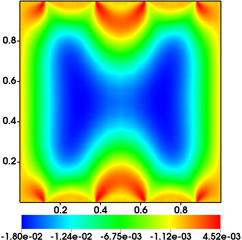
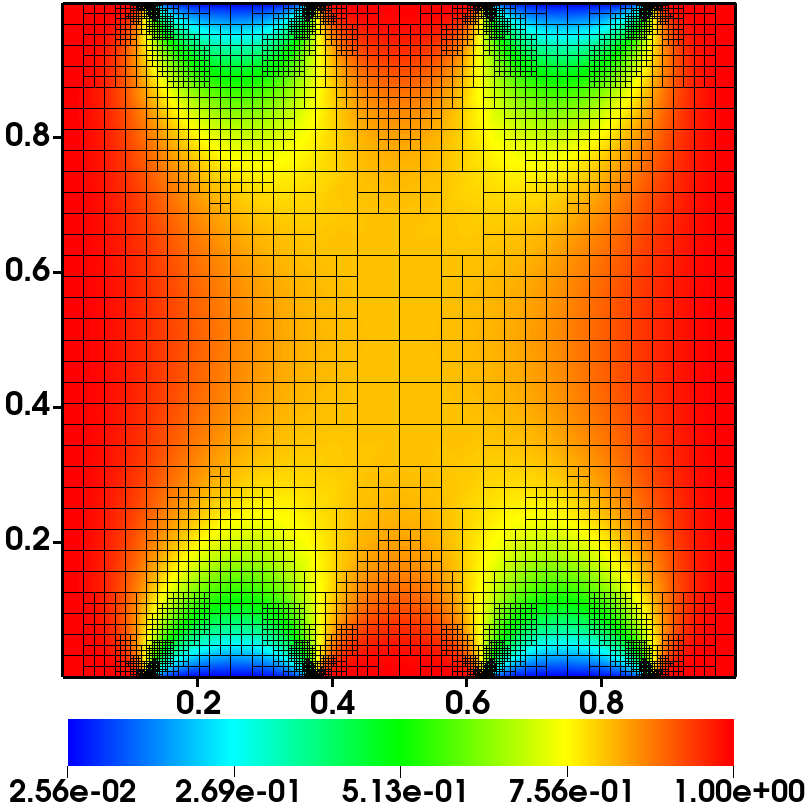
The effects of the large electric field are seen in Figure 2(2(a)), which shows the computed solution on the finest mesh with Dorfler AMR. In response to the field, the director deforms to align with the field lines, even near the boundary where elastic resistance is strongest. The electric potential is illustrated in Figure 2(2(c)). The regions surrounding the rapid transitions in the electric potential contain the most difficult to resolve physics and the largest free-energy contributions. This suggests that a significant portion of the total approximation error will also be present in these areas. In Figure 2(2(b)), the refinement patterns clearly emphasize the transition regions. As such, finer mesh elements improve resolution therein while areas with dynamics that are likely already well captured by a coarser mesh, such as those near y=0y=0, are de-emphasized.

Refer to caption
(a)
Refer to caption
(b)
Refer to caption
(c)
Figure 2: (2(a)) Fine-mesh computed solution (restricted for visualization) using Dorfler AMR with ν=0.1\nu=0.1. (2(b)) Resulting mesh patterns after six levels of adaptive refinement overlaid on the value of n1n_{1}. (2(c)) Electric potential produced by the patterned surfaces and flexoelectric coupling.

In Table 3, the AMR solution exhibits slightly tighter unit-length conformance compared to the finest uniform mesh. Furthermore, the solution computed with AMR matches the free energy found with uniform refinement. As in the previous example, the sharp boundary conditions of the electric potential lead to relatively large Gauss’ law conformance values. However, conformance of the AMR solution is less than half that of the uniform mesh solution, indicating better physical law conformance. Furthermore, by each measure of computational cost, adaptive refinement yields significant reductions. The solves using AMR consume roughly 1212 times fewer WUs and produce solutions more than an order of magnitude faster.

Table 3: Statistics associated with the flexoelectric problem comparing solutions computed with AMR and Dorfler marking to those applying uniform refinement. Numbers correspond to each approaches finest mesh. The first two columns are the largest director deviations above and below unit-length at the quadrature nodes. The third column is the free energy, as expressed in Equation (1). “Gauss” quantifies a solutions conformance to Gauss’ law.
Strategy Pos. Dev. Neg. Dev. Energy Gauss DOFs WUs Time
Uniform 4.4474.447e-0202 2.7002.700e-0202 −38.0412-38.0412 110.417110.417 4,202,5004,202,500 4.7204.720 1,8761,876s
Adaptive 4.4394.439e-0202 2.6952.695e-0202 −38.0412-38.0412 37.13037.130 336,628336,628 0.3840.384 57.257.2s

Statistics associated with the hierarchy of NI meshes are reported in Table 4. While the DOFs scale much more rapidly with uniform refinement, the computed free energies remain comparable. As in the previous experiment, AMR solutions yield similar H1 errors compared to the uniform mesh solutions with significantly less DOFs. For instance, the seventh AMR solutions yields a smaller H1 error while using nearly 5050 times fewer DOFs than the finest uniform mesh. It should be noted that as error becomes more equally distributed, uniform refinement on subsequent meshes emerges as the optimal strategy. However, a maximum proportion of (1−ν)(1-\nu) cells may be refined at a given level with Dorfler marking, preventing fully uniform refinement for a given mesh. As an illustration of this phenomenon, a final step of uniform refinement in the “Adaptive” run, delineated as Mesh 8∗, is performed. This refinement cuts the error by nearly 80%, far outpacing the error of the finest uniform mesh while still utilizing an order of magnitude fewer DOFs.

Table 4: A comparison of the DOFs, Newton steps required for convergence, free energy, and H1 error (relative to the overkill solution) across the NI hierarchy for uniform and adaptive mesh refinement, respectively. H1 Est. denotes the total estimator across all elements and ΘT\Theta_{T} represents the maximum estimator value for each mesh.
Strategy Uniform Adaptive
Mesh DOFs Steps Energy H1 Error DOFs Steps Energy H1 Error H1 Est. ΘT\Theta_{T}
1 4,3564,356 108108 −34.4431-34.4431 3.418323.41832 4,3564,356 108108 −34.4431-34.4431 3.418323.41832 54.55354.553 25.11125.111
2 16,90016,900 4444 −37.3751-37.3751 1.600861.60086 4,9724,972 4545 −37.3177-37.3177 1.672761.67276 36.37936.379 16.38216.382
3 66,56466,564 1515 −38.0264-38.0264 0.572710.57271 6,0526,052 1515 −38.0143-38.0143 0.622420.62242 19.45419.454 8.0198.019
4 264,196264,196 88 −38.0354-38.0354 0.155940.15594 8,4168,416 88 −38.0318-38.0318 0.203740.20374 7.4957.495 2.1462.146
5 1,052,6761,052,676 33 −38.0402-38.0402 0.048030.04803 15,35615,356 44 −38.0394-38.0394 0.076030.07603 2.6922.692 0.3660.366
6 4,202,5004,202,500 33 −38.0412-38.0412 0.013470.01347 35,18035,180 33 −38.0410-38.0410 0.028220.02822 1.0521.052 0.0610.061
7 – – – – 86,70086,700 22 −38.0412-38.0412 0.010380.01038 0.1680.168 0.0040.004
8∗ – – – – 336,628336,628 22 −38.0412-38.0412 0.002350.00235 – –

6 Conclusion and Future Work

In this work, we have discussed an a posteriori error estimator for the electrically and flexoelectrically coupled Frank-Oseen models of nematic liquid crystals with the necessary unit-length constraint enforced via a penalty method. It was shown that the proposed coupled estimator provides a reliable estimate of global approximation error and is an efficient indicator of local error. The estimator is comprised of readily computable, local quantities suitable for use as part of standard cell flagging schemes, including Dorfler marking. Finally, numerical results suggest that it is highly effective in guiding AMR as part of a multilevel nested iteration framework. For each numerical experiment considering flexoelectrically coupled problems with challenging applied electric fields or boundary conditions, AMR with NI produces solutions of better quality and significant reductions in computational cost along a number of metrics. Future work will include extending the theoretical framework to demonstrate reliability and efficiency of the error estimator associated with a Lagrange multiplier formulation. Further, studies incorporating novel multigrid schemes and marking strategies will also be considered. Work investigating whether the present theory can be extended to support irregular meshes, such as those with hanging nodes, as considered in the numerical experiments, is also planned.

Acknowledgments

The authors would like to thank Professor Xiaozhe Hu for his helpful suggestions, guidance, and compute resources for the overkill solutions. We would also like to thank Divya Sivasankaran for her careful reading of the manuscript. Finally, thank you to the anonymous reviewers whose suggestions improved this work.

References

  • [1] J. H. Adler, T. J. Atherton, T. R. Benson, D. B. Emerson, and S. P. MacLachlan, Energy minimization for liquid crystal equilibrium with electric and flexoelectric effects, SIAM J. Sci. Comput., 37 (2015), pp. S157–S176.
  • [2] J. H. Adler, D. B. Emerson, S. P. MacLachlan, and T. A. Manteuffel, Constrained optimization for liquid crystal equilibria, SIAM J. Sci. Comput., 38 (2016), pp. B50–B76.
  • [3] T. J. Atherton and J. R. Sambles, Orientational transition in a nematic liquid crystal at a patterned surface, Phys. Rev. E, 74 (2006).
  • [4] I. Babuska and W. C. Rheinboldt, A posteriori error estimates for the finite element method, Int. J. Numer. Meth. Engng, (1978), pp. 1597–1615.
  • [5] W. Bangerth, R. Hartmann, and G. Kanschat, deal.II – a general purpose object oriented finite element library, ACM Trans. Math. Softw., 33 (2007), pp. 24/1–24/27.
  • [6] R. E. Bank and D. B. Welfert, A posteriori error estimators for elliptic partial differential equations, Math. Comp., 44 (1985), pp. 283–301.
  • [7] S. C. Brenner and L. Scott, The Mathematical Theory of Finite Element Methods, Springer-Verlag, 1996.
  • [8] P. Clément, Approximation by finite element functions using local regularization, RAIRO Anal. Numér., 2 (1975), pp. 77–84.
  • [9] M. G. Clerk, E. Vidal-Henriquez, J. D. Davila, and M. Kowalczyk, Symmetry breaking of nematic umbilical defects through an amplitude equation, Phys. Rev. E, 90 (2014).
  • [10] T. A. Davis and E. C. Gartland-Jr., Finite element analysis of the Landau-de Gennes minimization problem for liquid crystals, SIAM J. Numer. Anal., 35 (1998), pp. 336–362.
  • [11] W. Döfler, A convergent adaptive algorithm for Poisson’s equation, SIAM J. Numer. Anal., 33 (1996), pp. 1106–1124.
  • [12] D. B. Emerson, A posteriori error estimates for the Frank-Oseen model of liquid crystals, J. Coupled Syst. Multiscale Dyn., 5 (2017), pp. 95–110.
  • [13] D. B. Emerson, J. H. Adler, P. E. Farrell, and S. P. MacLachlan, Combining deflation and nested iteration for computing multiple solutions of nonlinear variational problems, SIAM J. Sci. Comput., 39 (2017), pp. B29–B52.
  • [14] E. C. Gartland-Jr., Scalings and limits of the Landau-de Gennes model for liquid crystals: A comment on some recent analytical papers. arXiv:1512.08614, 2015.
  • [15] J. Harden, M. Chambers, R. Verduzco, P. Luchette, J. T. Gleeson, S. Sprunt, and A. Jákli, Giant flexoelectricity in bent-core nematic liuqid crystal elastomers, Appl. Phys. Lett., 96 (2010).
  • [16] V. John, Residual a posteriori error estimates for two-level finite element methods for the Navier-Stokes equations, Appl. Numer. Math., (2001), pp. 503–518.
  • [17] J. P. F. Lagerwall and G. Scalia, A new era for liquid crystal research: Applications of liquid crystals in soft matter, nano-, bio- and microtechnology, Curr. Appl. Phys., 12 (2012), pp. 1387–1412.
  • [18] B. W. Lee and N. A. Clark, Alignment of liquid crystals with patterned isotropic surfaces, Science, 291 (2001), pp. 2576–2580.
  • [19] R. B. Meyer, Piezoelectric effects in liquid crystals, Phys. Rev. Lett., 22 (1969), pp. 918–921.
  • [20] J. T. Oden, W. Wu, and M. Ainsworth, An a posteriori error estimate for finite element approximations of the Navier-Stokes equations, Comput. Methods Appl. Mech. Engrg, (1994), pp. 185–202.
  • [21] L. Onsager, The effects of shape on the interaction of colloidal particles, Ann. NY Acad. Sci., 51 (1949), pp. 627–659.
  • [22] O. A. Rojas-Gómez, J. M. Romero-Enrique, N. M. Silvestre, and M. M. T. da Gama, Pattern-induced anchoring transitions in nematic liquid crystals, J. Phys. Condens. Matter, 29 (2017).
  • [23] G. Starke, Gauss-Newton multilevel methods for least-squares finite element computations of variably saturated subsurface flow, Computing, 64 (2000), pp. 323–338.
  • [24] I. W. Stewart, The Static and Dynamic Continuum Theory of Liquid Crystals: A Mathematical Introduction, Taylor and Francis, London, 2004.
  • [25] R. Verfürth, A posteriori error estimators for the Stokes equations, Numer. Math., 55 (1989), pp. 309–325.
  • [26]  , A posteriori error estimates for nonlinear problems. Finite element discretizations of elliptic equations, Math. Comp., 62 (1994), pp. 445–475.
  • [27]  , A Posteriori Error Estimation Techniques for Finite Element Methods, Oxford University Press, 2013.
  • [28] E. G. Virga, Variational Theories for Liquid Crystals, Chapman and Hall, London, 1994.
  • [29] Y. Wan and D. Zhao, On the controllable soft-templating approach to mesoporous silicates, Chem. Rev., 107 (2007), pp. 2821–2860.