跳到论文正文
W Papers独立论文阅读器 arXiv:2304.01972 论文正文 计算阅读时间 · 0%
引用这篇论文根据当前论文元数据生成,正式投稿前建议核对。


License: arXiv.org perpetual non-exclusive license
arXiv:2304.01972v1 [cs.IT] 04 Apr 2023

An Information-Theoretic Approach to Collaborative Integrated Sensing and Communication for Two-Transmitter Systems

Mehrasa Ahmadipour and Michèle Wigger Affiliation: 1 LTCI Telecom Paris, IP Paris, 91120 Palaiseau, France, Emails: {mehrasa.ahmadipour,michele.wigger}@telecom-paris.fr
Abstract

This paper considers information-theoretic models for integrated sensing and communication (ISAC) over multi-access channels (MAC) and device-to-device (D2D) communication. The models are general and include as special cases scenarios with and without perfect or imperfect state-information at the MAC receiver as well as causal state-information at the D2D terminals. For both setups, we propose collaborative sensing ISAC schemes where terminals not only convey data to the other terminals but also state-information that they extract from their previous observations. This state-information can be exploited at the other terminals to improve their sensing performances. Indeed, as we show through examples, our schemes improve over previous non-collaborative schemes in terms of their achievable rate-distortion tradeoffs. For D2D we propose two schemes, one where compression of state information is separated from channel coding and one where it is integrated via a hybrid coding approach.

I Introduction

Next-generation wireless networks are expected to support several autonomous and intelligent applications that rely heavily on accurate sensing and localization techniques [1]. Important examples are intelligent transport systems, where vehicles continuously sense environmental changes and simultaneously exchange sensing-information and data with already detected vehicles, base stations, or central servers. Such simultaneous sensing and data-communication applications are also the focus of this work. More specifically, we are interested in multi-terminal scenarios where different terminals communicate data with each other and simultaneously exploit the backscattered signals for sensing purposes.

A common but naive approach to address sensing and communication is to separate the two tasks in independent systems and split the available resources such as bandwidth and power between the two systems. In our information-theoretic model, such a system corresponds to resource-sharing (e.g., time-sharing) between communication and sensing. However, the high cost of spectrum and hardware encourages integrating the sensing and communications tasks via a single waveform and a single hardware platform [2, 3]. A large body of works studied integrated sensing and communication (ISAC) scenarios from a communication-theoretic or signal-processing perspective (see, e.g., [4, 5] and references therein), mostly investigating appropriate choices for the employed waveform that in ISAC applications has to serve both the sensing and the communication tasks. Interestingly, different tradeoffs between the communication and sensing performances can be obtained by changing the employed waveform.

The fundamental performance limits of integrated sensing and communication systems were first considered in [6]. Specifically, [6] introduced an information-theoretic model for integrated sensing and communication based on a generalized-feedback model, which captures two underlying assumptions used in radar signal processing. On the one hand, generalized feedback captures the inherently passive nature of the backscattered signal observed at the transmitter (Tx), which cannot be controlled but is determined by its surrounding environment. On the other hand, it models the fact that the backscattered signal depends on the waveform employed by the Tx. It was proposed to use the classical average per-letter block-distortion to measure the Tx’s sensing performance on the i.i.d. state-sequence. The authors of [6], see also [7] characterized the exact capacity-distortion tradeoff of arbitrary discrete memoryless channels (DMCs) with generalized feedback. This quantity naturally measures the inherent tradeoff between increasing data rate and reducing sensing distortion in such integrated systems. Interestingly, the results show that the optimal tradeoff is achieved by standard random code constructions as used for traditional data communication, where the statistics of the channel inputs (and thus of the codewords) however has to be adapted to meet the desired sensing performance. Notice that this observation is consistent with the signal-processing literature on the search for adequate channel input waveforms which allow to meet the desired sensing performance while still achieving high communication rates. Similar results were also derived for discrete memoryless broadcast channels (DMBCs) [7] where a single transmitter communicates with two receivers. Both the DMC and the DMBC are thus single-Tx networks, and the optimal sensing is a simple per-symbol estimation of the hidden state given the channel inputs and outputs at the sensing terminal. The optimality of such a simple symbol-by-symbol estimator stems from the fact that for a fixed input sequence the generalized feedback channels and the state-sequence both behave in a memoryless manner.

The sensing situation becomes more interesting and challenging when the sensing terminal is not the only terminal feeding inputs to the channel. In this case, the effective disturbance for the sensing is not necessarily memoryless since the inputs from the other terminals also create disturbances and can have memory. In this case, a strategy that first attempts to guess the other Txs’ codewords followed by a symbol-wise estimator based on the observations and the guessed codewords can lead to a smaller (and thus better) distortion. This has also been observed in [8], where communication is over a DMC and state estimation is performed at the receiver (Rx) side. In this case, the optimal sensing strategy is first to decode the Tx’s codeword and then apply an optimal symbol-by-symbol estimator to this codeword and the observed channel outputs. A similar strategy was applied in the two-transmitter single-Rx multi-access channel (MAC) ISAC scenario of [9] where through the generalized feedback each Tx first decodes part of the data sent by the other Tx and then applies a symbol-by-symbol estimator to the decoded codeword as well as its own channel inputs and outputs. In fact, the ISAC scheme of [9] is based on Willems’ scheme for the MAC with generalized feedback, where each Tx encodes its data into two super-positioned codewords, whereof the lower data-layer is decoded by the other Tx. This data is then repeated by both Txs in the next block as part of a third lowest-layer codeword, allowing the two Txs to transmit data cooperatively Somewhat naturally, [9] suggests to use this decoded lower data-layer also for sensing purposes in the sense that each Tx applies the symbol-by-symbol estimator not only to its inputs and outputs but also to this decoded codeword. In this article, which is based on the conference paper [10], we suggest to use this decoded codeword not only to exchange data,but also to exchange sensing information. The concept of exchanging sensing information for ISAC has been studied in the signal processing literature under the paradigm of collaborative sensing.

In this sense, we introduce the concept of collaborative sensing for ISAC also to the information-theoretic literature, where we focus on the MAC and the related device-to-device (D2D) communication, i.e., the two-way channel. For the MAC, we naturally extend Willem’s coding scheme so as to convey also state-information from one Tx to the other over the communication path that is built over the generalized feedback link. The proposed scheme can be considered as a separate source-channel coding scheme in the sense that each Tx first compresses the obtained outputs and inputs so as to extract state information, and then transmits the compression index using a pure channel code (here Willems’ coding scheme) to the other Tx. The proposed scheme obtains a better sensing performance than a previous ISAC scheme [9] without collaborative sensing, and thus a better distortion-capacity tradeoff. For D2D communication, we present a similar collaborative sensing ISAC scheme based on source-channel separation and using Han’s two-way channel scheme. Furthermore, we present an improved scheme that is based on joint source-channel coding (JSCC), more specifically on hybrid coding. We show enhanced performances of both simple collaborative sensing schemes. In both the MAC and the D2D scenario, the maximum rates achieved by our proposed scheme for given sensing distortions are strictly concave functions of the distortion pairs, and thus also improve over classical time- or resource-sharing strategies.

Recently, various other information-theoretic works have analyzed the fundamental limits of ISAC systems, such as [11, 12, 13, 14]. For example, [14] analyzes systems with secrecy constraints, while [11, 12, 13] study channels that depend on a single fixed parameter and transmitters or sensor nodes wish to estimate this parameter based on backscatter signals. Their model is thus suited for scenarios where the estimation parameters change at a much slower time scale compared to the channel symbol period. Specifically, while in [12] sensing (parameter estimation) is performed at the transmitter, in [11] it is performed at a sensor that is close but not collocated with the transmitter. The study in[13] analyzes the detection-error exponents of open-loop and close-loop coding strategies.

Summary of Contributions and Outline of this Article:

  • •

    In Section II we introduce our information-theoretic ISAC MAC model with state-sensing at the Txs. We also show that it is of general nature and in particular can model scenarios with partial or perfect channel state information at the Rx as well as scenarios where the Txs wish to reconstruct functions or distorted versions of the actual state that is governing the channel.

  • •

    In Section III we describe our collaborative-sensing ISAC MAC scheme and show at hand of examples that it improves both over simple time-sharing as well as over previous schemes. Notice that our scheme does not employ Wyner-Ziv compression, but the equally strong implicit binning technique, as used for example in [15].

  • •

    Section IV describes our information-theoretic ISAC D2D model with state-sensing at both terminals. Again, we show that our model is rather general and includes scenarios with strictly-causal perfect or imperfect state-information at the terminals.

  • •

    In Section V we propose two collaborative-sensing ISAC D2D schemes. The first is based on a separate source-channel coding approach and the second on an improved JSCC approach using hybrid coding. In both schemes, the transmitted codeword carries not only data but also compression information that the other terminal can exploit for sensing. While the separation-based scheme employs Wyner-Ziv compression to account for the side-information at the other Tx, the JSCC based scheme uses implicity binning as in standard hybrid coding.

Notations: We use calligraphic letters to denote sets, e.g., 𝒳{\cal X}. Random variables are denoted by uppercase letters, e.g., XX, and their realizations by lowercase letters, e.g., xx. For positive integers nn, we use [1:n][1:n] to denote the set {1,⋯,n}\{1,\cdots,n\}, XnX^{n} for the tuple of random variables (X1,⋯,Xn)(X_{1},\cdots,X_{n}) and xnx^{n} for (x1,…,xn)(x_{1},\ldots,x_{n}). We abbreviate independent and identically distributed as i.i.d. and probability mass function as pmf. Logarithms are taken with respect to base 22. We shall use 𝒯ϵN​(PX​Y){\cal T}_{\epsilon}^{N}(P_{XY}) to indicate the of strongly jointly-typical sequences {(xn,yn)}\{(x^{n},y^{n})\} with respect to the distribution PX​YP_{XY} as defined in [16]. For an index k∈{1,2}k\in\{1,2\}, we define k¯:=3−k\bar{k}:=3-k and for an event 𝒜\mathcal{A} we denote its complement by 𝒜¯\bar{\mathcal{A}}. Moreover, 𝟙​{⋅}\mathbbm{1}\{\cdot\} denotes the indicator function.

II Two-User Multiple-Access Channel with Generalized Feedback: System Model

In this section we consider the two-user multi-access channel (MAC) with generalized feedback, where two Txs wish to convey independent data to a common Rx and through the generalized feedback link they estimate the respective state sequences S1nS_{1}^{n} and S2nS_{2}^{n} governing the transition law over the MAC and the generalized feedback.

II-A System Model

Consider the two-Tx single-Rx MAC scenario in Fig. 1. The model consists of a two-dimensional memoryless state sequence {(S1,i,S2,i)}i≥1\{(S_{1,i},S_{2,i})\}_{i\geq 1} whose samples at any given time ii are distributed according to a given joint law PS1​S2P_{S_{1}S_{2}} over the state alphabets 𝒮1×𝒮2{\cal S}_{1}\times{\cal S}_{2}. Given that at time-ii Tx 1 sends input X1,i=x1X_{1,i}=x_{1} and Tx 2 input X2,i=x2X_{2,i}=x_{2} and given state realizations S1,i=s1S_{1,i}=s_{1} and S2,i=s2S_{2,i}=s_{2}, the Rx’s time-ii output YiY_{i} and the Txs’ feedback signals Z1,iZ_{1,i} and Z2,iZ_{2,i} are distributed according to the time-invariant channel transition law PY​Z1​Z2|S1​S2​X1​X2(⋅,⋅,⋅|s1,s2,x1,x2)P_{YZ_{1}Z_{2}|S_{1}S_{2}X_{1}X_{2}}(\cdot,\cdot,\cdot|s_{1},s_{2},x_{1},x_{2}). Input and output alphabets 𝒳1,𝒳2,𝒴,𝒵1,𝒵2,𝒮1,𝒮2{\cal X}_{1},{\cal X}_{2},{\cal Y},{\cal Z}_{1},{\cal Z}_{2},{\cal S}_{1},{\cal S}_{2} are assumed finite.11 1 Notice that our results can also be extended to well-behaved continuous channels.

Fig. 1: State-dependent discrete memoryless multiaccess channel with sensing at the transmitters.

A (2n​𝖱1,2n​𝖱2,n)(2^{n\mathsf{R}_{1}},2^{n\mathsf{R}_{2}},n)-code consists of

  1. 1.

    two message sets 𝒲1=[1:2n​𝖱1]{\cal W}_{1}=[1:2^{n\mathsf{R}_{1}}] and 𝒲2=[1:2n​𝖱2]{\cal W}_{2}=[1:2^{n\mathsf{R}_{2}}];

  2. 2.

    a sequence of encoding functions Ωk,i:𝒲k×𝒵ki−1→𝒳k\Omega_{k,i}\colon{\cal W}_{k}\times{\cal Z}_{k}^{{i-1}}\to{\cal X}_{k}, for i=1,2,…,ni=1,2,\ldots,n and k=1,2k=1,2;

  3. 3.

    a decoding function g:𝒴n→𝒲1×𝒲2g\colon{\cal Y}^{n}\to{\cal W}_{1}\times{\cal W}_{2};

  4. 4.

    for each k=1,2k=1,2 a state estimator ϕk:𝒳kn×𝒵kn→𝒮^kn\phi_{k}\colon{\cal X}_{k}^{n}\times{\cal Z}_{k}^{n}\to\hat{{\cal S}}_{k}^{n}, where 𝒮^1\hat{{\cal S}}_{1} and 𝒮^2\hat{{\cal S}}_{2} are given reconstruction alphabets.

Fix a blocklength nn, rates R1,R2≥0R_{1},R_{2}\geq 0, and a (2n​R1,2n​R2,n)(2^{nR_{1}},2^{nR_{2}},n)-code ({Ω1,i},{Ω2,i},g,ϕ1,ϕ2)(\{\Omega_{1,i}\},\{\Omega_{2,i}\},g,\phi_{1},\phi_{2}). Let then the random message WkW_{k} be uniformly distributed over the message set 𝒲k{\cal W}_{k}, for each k=1,2k=1,2, and the generate the inputs according to the encoding function Xk,i=Ωk,i​(Wk,Zki−1)X_{k,i}=\Omega_{k,i}(W_{k},Z_{k}^{i-1}), for i=1,…,ni=1,\ldots,n. The Txs’ state estimates are obtained as S^kn:=(S^k,1,⋯,S^k,n)=ϕk​(Xkn,Zkn)\hat{S}_{k}^{n}:=(\hat{S}_{k,1},\cdots,\hat{S}_{k,n})=\phi_{k}(X_{k}^{n},Z_{k}^{n}) and the Rx’s guess of the messages as (W^1,W^2)=g⁡(Yn)(\hat{W}_{1},\hat{W}_{2})=g(Y^{n}). We shall measure the quality of the state estimates S^kn\hat{S}_{k}^{n} by bounded per-symbol distortion functions dk:𝒮k×𝒮^k↦[0,∞)d_{k}\colon{\cal S}_{k}\times\hat{{\cal S}}_{k}\mapsto[0,\infty), and consider expected average block distortions

Δk(n):=1n∑i=1n𝔼[dk(Sk,i,S^k,i)],k=1,2.\Delta_{k}^{(n)}:=\frac{1}{n}\sum_{i=1}^{n}\mathbb{E}[d_{k}(S_{k,i},\hat{S}_{k,i})],\quad k=1,2. (1)

The probability of decoding error is defined as:

Pe(n)\displaystyle P^{(n)}_{e} :⁣=\displaystyle:= Pr​(W^1≠W1,or,W^2≠W2).\displaystyle\textnormal{Pr}\Big(\hat{W}_{1}\neq W_{1}\quad\textnormal{or}\quad\hat{W}_{2}\neq W_{2}\Big). (2)
Definition 1.

A rate-distortion tuple (𝖱1,𝖱2,𝖣1,𝖣2)(\mathsf{R}_{1},\mathsf{R}_{2},\mathsf{D}_{1},\mathsf{D}_{2}) is achievable if there exists a sequence (in nn) of (2n​𝖱1,2n​𝖱2,n)(2^{n\mathsf{R}_{1}},2^{n\mathsf{R}_{2}},n) codes that simultaneously satisfy

limn→∞Pe(n)\displaystyle\lim_{n\to\infty}P^{(n)}_{e} =\displaystyle= 0\displaystyle 0 (3a)
lim¯n→∞⁡Δk(n)\displaystyle\varlimsup_{n\to\infty}\Delta_{k}^{(n)} ≤\displaystyle\leq 𝖣k,for ​k=1,2.\displaystyle\mathsf{D}_{k},\quad\textnormal{for }k=1,2. (3b)
Definition 2.

The capacity-distortion region 𝒞𝒟{\cal{CD}} is the closure of the set of all achievable tuples (𝖱1,𝖱2,𝖣1,𝖣2)(\mathsf{R}_{1},\mathsf{R}_{2},\mathsf{D}_{1},\mathsf{D}_{2}).

Remark 1 (On the States).

Notice that the general law PS1​S2P_{S_{1}S_{2}} governing the states S1nS_{1}^{n} and S2nS_{2}^{n} allows to model various types of situations including scenarios where the state sequences are highly correlated (even identical) or scenarios where the state-sequences are independent.

Our model also includes a scenario where the channel is governed by an internal i.i.d. state sequence SnS^{n} of pmf PSP_{S} and the states S1n,S2nS_{1}^{n},S_{2}^{n} are related to SnS^{n} over an independent memoryless channel PS1​S2|SP_{S_{1}S_{2}|S}. For example, the states S1nS_{1}^{n} and S2nS_{2}^{n} can be imperfect or noisy versions of the actual state sequence SnS^{n}. To see that this scenario can be included in our model, notice that since no terminal observes SnS^{n} nor attempts to reconstruct SnS^{n}, both the distortions and the error probabilities only depend on the conditional law

PY​Z1​Z2|X1​X2​S1​S2(y,z1,z2|x1,x2,s1,s2)\displaystyle P_{YZ_{1}Z_{2}|X_{1}X_{2}S_{1}S_{2}}(y,z_{1},z_{2}|x_{1},x_{2},s_{1},s_{2}) =\displaystyle= (4)
∑sPY​Z1​Z2|X1​X2​S(y,z1,z2|x1,x2,s)PS​(s)​PS1​S2|S​(s1,s2|s)PS1​S2​(s1,s2),\displaystyle\hskip-56.9055pt\sum_{s}P_{YZ_{1}Z_{2}|X_{1}X_{2}S}(y,z_{1},z_{2}|x_{1},x_{2},s)\frac{P_{S}(s)P_{S_{1}S_{2}|S}(s_{1},s_{2}|s)}{P_{S_{1}S_{2}}(s_{1},s_{2})},

where PS1​S2​(s1,s2)=∑sPS​(s)​PS1​S2|S​(s1,s2|s)P_{S_{1}S_{2}}(s_{1},s_{2})=\sum_{s}P_{S}(s)P_{S_{1}S_{2}|S}(s_{1},s_{2}|s) denotes the joint pmf of the two states. Computing the channel law in (4) and plugging it into our results in the next section, thus immediately also provides results for the described setup where the actual state is SnS^{n} and the states S1nS_{1}^{n} and S2nS_{2}^{n} are noisy versions thereof.

Remark 2 (State-Information).

Our model also includes scenarios with perfect or imperfect state-information at the Rx. In fact, considering our model with an output

Y=(T,Y′)Y=(T,Y^{\prime}) (5)

where Y′Y^{\prime} denotes the actual MAC output and TT the Rx’s imperfect channel state-information about the states S1nS_{1}^{n} and S2nS_{2}^{n} . Notice that in our model, the Rx observes the state-information TnT^{n} only in a causal manner. Causality is however irrelevant here since the Rx only has to decode the messages at the end of the entire transmission. Therefore, plugging the choice (5) into our results for TT the Rx state-information and Y′Y^{\prime} the actual MAC output, our results in the following section directly lead to results for this related setup with Rx state-information.

Remark 3 (The Relay-Channel).

The MAC with generalized-feedback model includes the relay-channel as a special case. It suffices to restrict R2=0R_{2}=0, in which case Tx 2 degenerates to a relay terminal. The results we elaborate in the following section does immediately apply also to the relay channel.

III A Collaborative ISAC Scheme for the MAC

Before describing our collaborative ISAC scheme for the MAC, we review literature on the MAC and in particular Willem’s scheme for the MAC with generalized feedback, which acts as a building block for our scheme.

While the capacity region of the MAC without feedback was determined in [17, 18], single-letter expressions for the capacity are only known in special cases such as the two-user Gaussian MAC with perfect feedback [19] or a class of semi-deterministic MACs [20] with one-sided perfect feedback. In [21], Kramer derived a multi-letter characterization of the capacity region of a general MAC with perfect feedback. For most channels it seems however challenging to evaluate this multi-letter characterization even numerically. In contrast, various inner and outer bounds on the capacity region of the MAC with generalized or perfect feedback are known. Outer bounds are typically based on the dependence balance bound idea by Hekstra and Willems [22], see also [23]. Various inner bounds were proposed based on schemes that each Tx decodes part of the data sent by the other Tx, which allows the two Txs to cooperatively resend these data parts in the next block using a more efficient coding scheme, see [24, 25, 26, 27, 22]. The one most relevant to our work is Willems’s inner bound [25], which we explain in more detail in the following subsection.

III-A Willems’ Coding Scheme with Generalized Feedback and the ISAC extension

Fig. 2: Operations at Tx 1 in Willems’ scheme during the first three blocks. After each block bb Tx 1 decodes message W2,c,(b)W_{2,c,(b)} based on its generalized feedback output Z1,(b)NZ_{1,(b)}^{N}. The decoded message is then retransmitted in block b+1b+1 jointly with W1,c,(b)W_{1,c,(b)}.

Willems’ scheme splits the blocklength nn into B+1B+1 blocks of length N=n/(B+1)N=n/(B+1) each. Accordingly, throughout, we let X1,(b)N,X2,(b)N,S1,(b)N,S2,(b)N,Z1,(b)N,Z2,(b)N,Y(b)NX_{1,(b)}^{N},X_{2,(b)}^{N},S_{1,(b)}^{N},S_{2,(b)}^{N},Z_{1,(b)}^{N},Z_{2,(b)}^{N},Y_{(b)}^{N} denote the block-bb inputs, states and outputs, e.g., S1,(b)N:=(S1​(b−1)​N+1,…,S1,b​N)S_{1,(b)}^{N}:=(S_{1(b-1)N+1},\ldots,S_{1,bN}). We also represent the two messages W1W_{1} and W2W_{2} in a one-to-one way as the 2​B2B-length tuples

Wk=(Wk,c,(1),…,Wk,c,(B),Wk,p,(1),…,Wk,p,(B)),k∈{1,2},W_{k}=(W_{k,c,(1)},\ldots,W_{k,c,(B)},W_{k,p,(1)},\ldots,W_{k,p,(B)}),\qquad k\in\{1,2\}, (6)

where all pairs (Wk,c,(b),Wk,p,(b))(W_{k,c,(b)},W_{k,p,(b)}) are independent and uniformly distributed over [2N​R¯k,c]×[2N​R¯k,p]\left[2^{N\bar{R}_{k,c}}\right]\times\left[2^{N\bar{R}_{k,p}}\right] for R¯k,c≜B+1B​Rk,c\bar{R}_{k,c}\triangleq\frac{B+1}{B}R_{k,c} and R¯k,p≜B+1B​Rk,p\bar{R}_{k,p}\triangleq\frac{B+1}{B}R_{k,p} and Rk,c+Rk,p=RkR_{k,c}+R_{k,p}=R_{k}.

An independent superposition code is constructed for each block bb (see also Figure 2):

  • •

    A lowest-level code 𝒞0,(b)\mathcal{C}_{0,(b)} consisting of 2N​R¯1,c⋅2N​R¯2,c2^{N\bar{R}_{1,c}}\cdot 2^{N\bar{R}_{2,c}} codewords u0,(b)​(w1,c,w2,c)u_{0,(b)}(w_{1,c},w_{2,c}) is constructed by drawing all entries i.i.d. according to a auxiliary pmf PU0P_{U_{0}}.

  • •

    At the lowest level of encoding, we apply superposition coding to combine two codebooks {uk,(b)N​(wk,c′∣w1,c,w2,c)}\{u^{N}_{k,(b)}(w^{\prime}_{k,c}\mid w_{1,c},w_{2,c})\} onto each codeword u0,(b)N​(w1,c,w2,c)u_{0,(b)}^{N}(w_{1,c},w_{2,c}), for k∈{1,2}k\in\{1,2\} and wk,c′∈[2N​Rk,c]w^{\prime}_{k,c}\in[2^{NR_{k,c}}], by drawing the ii-th entry of each codeword according to PUk|U0(⋅∣u0)P_{U_{k}\mid U_{0}}(\cdot\mid u_{0}) where u0u_{0} denotes the ii-th entry of u0N​(w1,c,w2,c)u_{0}^{N}(w_{1,c},w_{2,c}).

  • •

    For each second-layer codeword uk,(b)N​(wk,c′|w1,c,w2,c)u^{N}_{k,(b)}(w^{\prime}_{k,c}|w_{1,c},w_{2,c}), we apply superposition coding by drawing the ii-th entry of a codebook xk,(b)N​(wk,p′|wk,c′,w1,c,w2,c){x_{k,(b)}^{N}(w_{k,p}^{\prime}|w_{k,c}^{\prime},w_{1,c},w_{2,c})} according to PXk|U0​Uk(⋅∣u0,uk)P_{X_{k}\mid U_{0}U_{k}}(\cdot\mid u_{0},u_{k}), where k∈1,2k\in{1,2} and wk,p′∈[2N​Rk,p]w^{\prime}_{k,p}\in[2^{NR_{k,p}}] and uku_{k} represents the ii-th entry of uk,(b)N​(wk,c′∣w1,c,w2,c)u^{N}_{k,(b)}(w^{\prime}_{k,c}\mid w_{1,c},w_{2,c}).

As depicted in Figure 2, in Willems’ scheme, Tx 11 sends the following block-bb channel inputs

x1,(b)N=x1,(b)N​(W1,p,(b)|W1,c,(b),W1,c,(b−1),W^2,c,(b−1)),b∈{1,…,B+1},x_{1,(b)}^{N}=x_{1,(b)}^{N}\left(W_{1,p,(b)}\Big|W_{1,c,(b)},W_{1,c,(b-1)},\hat{W}_{2,c,(b-1)}\right),\qquad b\in\{1,\ldots,B+1\}, (7)

where W^2,c,(b−1)\hat{W}_{2,c,(b-1)} denotes the message part that Tx 1 decodes after reception of the block-(b−1)(b-1) generalized feedback signal Z1,(b−1)NZ_{1,(b-1)}^{N}, e.g., through a joint typicality decoding rule. Also, we set throughout Wk,c,(0)=W^k,c,(0)=Wk,p,(B+1)=1{W}_{k,c,(0)}=\hat{W}_{k,c,(0)}=W_{k,p,(B+1)}=1, for k∈{1,2}k\in\{1,2\}.

Decoding at the Rx is performed backwards, starting with the last block B+1B+1 based on which the Rx decodes the pair of common messages (W1,c,(B),W2,c,(B))(W_{1,c,(B)},W_{2,c,(B)}) using for example a joint-typicality decoder. It then uses knowledge of these common messages and the outputs in block BB to decode the block-BB private messages (W1,p,(B),W2,p,(B))(W_{1,p,(B)},W_{2,p,(B)}) and the block (B−1)(B-1) common messages (W1,c,(B−1),W2,c,(B−1))(W_{1,c,(B-1)},W_{2,c,(B-1)}), etc. The backward decoding procedure is also depicted in Figure 3.

Fig. 3: Backward decoding procedure at the Rx in Willems’ scheme. The pair of common messages (W1,c,(b−1),W2,c,(b−1))(W_{1,c,(b-1)},W_{2,c,(b-1)}) and private messages (W1,p,(b),W2,p,(b))(W_{1,p,(b)},W_{2,p,(b)}) are jointly decoded based on the block-bb outputs Y(b)NY_{(b)}^{N} and using the previously decoded (W^1,c,(b),W^2,c,(b))(\hat{W}_{1,c,(b)},\hat{W}_{2,c,(b)}).

As Willems showed, his scheme can achieve the following rate-region.

Theorem 1 (Willems’ Achievable Region [25]).

Any nonnegative rate-pair (R1,R2)(R_{1},R_{2}) is achievable over the MAC with generalized feedback if it satisfies the following inequalities

Rk\displaystyle R_{k} ≤\displaystyle\leq I⁡(Xk;Y∣Xk¯​Uk​U0)+I⁡(Uk;Zk¯∣Xk¯​U0),k∈{1,2},\displaystyle I(X_{k};Y\mid X_{\bar{k}}U_{k}U_{0})+I(U_{k};Z_{\bar{k}}\mid X_{\bar{k}}U_{0}),\qquad k\in\{1,2\}, (8)
R1+R2\displaystyle R_{1}+R_{2} ≤\displaystyle\leq I⁡(X1​X2,Y),\displaystyle I(X_{1}X_{2};Y), (9)
R1+R2\displaystyle R_{1}+R_{2} ≤\displaystyle\leq I⁡(X1​X2;Y∣U0​U1​U2)+I⁡(U1;Z2∣X2​U0)+I⁡(U2;Z1∣X1​U0),\displaystyle I(X_{1}X_{2};Y\mid U_{0}U_{1}U_{2})+I(U_{1};Z_{2}\mid X_{2}U_{0})+I(U_{2};Z_{1}\mid X_{1}U_{0}), (10)

for some choice of pmfs PU0,PU1|U0,PU2|U0,PX1|U0​U1,PX2|U0​U2,P_{U_{0}},P_{U_{1}\mid U_{0}},P_{U_{2}\mid U_{0}},P_{X_{1}\mid U_{0}U_{1}},P_{X_{2}\mid U_{0}U_{2}}, and where above mutual informations are calculated according to the pmf PU0​PU1|U0​PU2|U0​PX1|U0​U1​PX2|U0​U2​PS1​S2P_{U_{0}}P_{U_{1}\mid U_{0}}P_{U_{2}\mid U_{0}}P_{X_{1}\mid U_{0}U_{1}}P_{X_{2}\mid U_{0}U_{2}}P_{S_{1}S_{2}} PY​Z1​Z2|S1​S2​X1​X2P_{YZ_{1}Z_{2}\mid S_{1}S_{2}X_{1}X_{2}}. One hereby can restrict to auxiliary variables over alphabets of sizes |𝒰k|≤(|𝒳k|+1)​|𝒰0||{\cal U}_{k}|\leq(|{\cal X}_{k}|+1)|{\cal U}_{0}|, for k=1,2k=1,2, and |𝒰0|≤|𝒳1|​|𝒳2|+1|{\cal U}_{0}|\leq|{\cal X}_{1}||{\cal X}_{2}|+1.

Kobayashi et al. [9] extended Willems’ scheme to a ISAC scenario by adding a state estimator at the two Txs. Specifically, for any block bb each Tx kk applies the symbol-per-symbol estimation

s^k,(b)N=ϕ~k∗⊗N(xk,(b)N,zk,(b)N,uk¯,(b)N(Wk¯,c,(b)|Wk,c,(b−1),W^k¯,c,(b−1))),b∈{1,…,B},\hat{s}_{k,(b)}^{N}=\tilde{\phi}_{k}^{*\otimes N}\left(x_{k,(b)}^{N},z_{k,(b)}^{N},u_{\bar{k},(b)}^{N}\left(W_{\bar{k},c,(b)}\ \Big|\ W_{k,c,(b-1)},\hat{W}_{\bar{k},c,(b-1)}\right)\right),\qquad b\in\{1,\ldots,B\}, (11)

where ϕ~k∗\tilde{\phi}_{k}^{*} denotes the optimal estimator of SkS_{k} based on the tuple (Xk,Zk,Uk¯)(X_{k},Z_{k},U_{\bar{k}}):

ϕ~k∗​(xk,zk,uk¯):=arg​min⁡∑sk∈𝒮ksk′∈𝒮k^⁡PSk|Xk​Zk​Uk¯​(sk|xk,zk,uk¯)​dk​(sk,sk′).\displaystyle\tilde{\phi}_{k}^{*}(x_{k},z_{k},u_{\bar{k}}):=\textnormal{arg}\min_{s_{k}^{\prime}\in\hat{\mathcal{S}_{k}}}\sum_{s_{k}\in\mathcal{S}_{k}}P_{S_{k}|X_{k}Z_{k}U_{\bar{k}}}(s_{k}|x_{k},z_{k},u_{\bar{k}})\;d_{k}(s_{k},s_{k}^{\prime}). (12)

Thus, any of the two Txs bases its state-estimation not only on its inputs and outputs of a given block but also on the codeword that it decoded from the other Tx.

For the last block B+1B+1, Tx kk can produce any trivial estimate, e.g., s^k,(B+1)N\hat{s}_{k,(B+1)}^{N} because its influence on the average distortion vanishes as the number of blocks grows, B→∞B\to\infty.

Combining the described state-estimation with Willems’ scheme, the following rate-distortion region can be shown to be achievable.

Theorem 2.

[Kobayashi et al.’s ISAC region [9]] A rate-distortion tuple (R1,R2,D1,D2)(R_{1},R_{2},D_{1},D_{2}) is achievable if it satisfies (8)–(10) and

E[dk(Sk,ϕ~k∗(Xk,Zk,Uk¯))]≤Dk,k=1,2,\displaystyle\textnormal{E}\Big[d_{k}\left(S_{k},{\color[rgb]{0,0,0}\tilde{\phi}_{k}^{*}\left(X_{k},Z_{k},U_{\bar{k}}\right)}\right)\Big]\leq D_{k},\quad k=1,2, (13)

for some choice of pmfs PU0,PU1|U0,PU2|U0,PX1|U1​U0,PX2|U2​U0P_{U_{0}},P_{U_{1}\mid U_{0}},P_{U_{2}\mid U_{0}},P_{X_{1}\mid U_{1}U_{0}},P_{X_{2}\mid U_{2}U_{0}}.

III-B Our Proposed Collaborative ISAC Scheme

We present our collaborative ISAC scheme. It extends the scheme in [9] in that the second-layer codeword of Willems’ code construction is not only used to transmit data but also compression information useful for state sensing. Each Tx generates compression information, which is primarily intended to be used by the other Tx to improve its sensing performance. In our scheme, the Rx however also decodes this information and uses it to improve its decoding performance.

Fig. 4: Our proposed scheme at Tx 1 during the firts three blocks

III-B1 Code construction

Choose pmfs PU0,PU1|U0​PU2|U0,PX1|U1​U0,PX2|U2​U0P_{U_{0}},P_{U_{1}\mid U_{0}}P_{U_{2}\mid U_{0}},P_{X_{1}\mid U_{1}U_{0}},P_{X_{2}\mid U_{2}U_{0}}, and define the pmf

PU0​U1​U2​X1​X2​S1​S2​Y​Z1​Z2​V1​V2\displaystyle P_{U_{0}U_{1}U_{2}X_{1}X_{2}S_{1}S_{2}YZ_{1}Z_{2}V_{1}V_{2}} =\displaystyle= PU0​PU1|U0​PU2|U0​PX1|U1​U0​PX2|U2​U0​PS1​S2​PY​Z1​Z2|X1​X2​S1​S2\displaystyle P_{U_{0}}P_{U_{1}\mid U_{0}}P_{U_{2}\mid U_{0}}P_{X_{1}\mid U_{1}U_{0}}P_{X_{2}\mid U_{2}U_{0}}P_{S_{1}S_{2}}P_{YZ_{1}Z_{2}\mid X_{1}X_{2}S_{1}S_{2}} (14)
PV1|X1​Z1​U2​U0​PV2|X2​Z2​U1​U0.\displaystyle\hskip 142.26378ptP_{V_{1}|X_{1}Z_{1}U_{2}U_{0}}{\color[rgb]{0,0,0}P_{V_{2}|X_{2}Z_{2}U_{1}U_{0}}}.

Employ Willems’ three-level superposition code construction for the given choice of pmfs, except that each second-layer codeword is indexed by a pair of indices. We thus denote the second-layer codewords by uk,(b)N(w1,c′,j1∣w1,c,w2,c)u^{N}_{k,(b)}(w^{\prime}_{1,c},j_{1}\mid w_{1,c},w_{2,c}) and u2,(b)N(w2,c′,j2∣w1,c,w2,c)u^{N}_{2,(b)}(w^{\prime}_{2,c},j_{2}\mid w_{1,c},w_{2,c}) and accordingly the corresponding third-layer codewords by x1,(b)N​(w1,p′|w1,c′,j1,w1,c,w2,c)x_{1,(b)}^{N}(w_{1,p}^{\prime}|w_{1,c}^{\prime},j_{1},w_{1,c},w_{2,c}) and x1,(b)N​(w2,p′|w2,c′,j2,w1,c,w2,c)x_{1,(b)}^{N}(w_{2,p}^{\prime}|w_{2,c}^{\prime},j_{2},w_{1,c},w_{2,c}), where the indices j1j_{1} and j2j_{2} take value in the sets [2n​R1′][2^{nR_{1}^{\prime}}] and [2n​R2′][2^{nR_{2}^{\prime}}] for some positive auxiliary rates R1,vR_{1,v} and R2,vR_{2,v}.

We further construct a compression codebook for each block and each of the two Txs, For each b∈{1,…,B}b\in\{1,\ldots,B\} and each sixtuple (w1,c,w2,c,w1,c′,j1​w2,c′,j2)∈[2N​R1,c]×[2N​R2,c]×[2N​R1,c]×[2N​R1,v]×[2N​R2,c]×[2N​R2,v](w_{1,c},w_{2,c},w^{\prime}_{1,c},j_{1}w^{\prime}_{2,c},j_{2})\in[2^{NR_{1,c}}]\times[2^{NR_{2,c}}]\times[2^{NR_{1,c}}]\times[2^{NR_{1,v}}]\times[2^{NR_{2,c}}]\times[2^{NR_{2,v}}] we generate a sequence v1,(b)N​(j1′∣w1,c′,j1,w2,c′,j2,w1,c,w2,c)v_{1,(b)}^{N}(j^{\prime}_{1}\mid w^{\prime}_{1,c},j_{1},w^{\prime}_{2,c},j_{2},w_{1,c},w_{2,c}) for each j1′∈[2N​R1,v]j_{1}^{\prime}\in[2^{NR_{1,v}}] and a sequence v2,(b)N​(j2′∣w1,c′,j1,w2,c′,j2,w1,c,w2,c)v_{2,(b)}^{N}(j^{\prime}_{2}\mid w^{\prime}_{1,c},j_{1},w^{\prime}_{2,c},j_{2},w_{1,c},w_{2,c}) for each j2′∈[2N​R2,v]j_{2}^{\prime}\in[2^{NR_{2,v}}]. The sequences v1,(b)N​(j1′∣w1,c′,j1,w2,c′,j2,w1,c,w2,c)v_{1,(b)}^{N}(j^{\prime}_{1}\mid w^{\prime}_{1,c},j_{1},w^{\prime}_{2,c},j_{2},w_{1,c},w_{2,c}) and v2,(b)N​(j2′∣w1,c′,j1,w2,c′,j2,w1,c,w2,c)v_{2,(b)}^{N}(j^{\prime}_{2}\mid w^{\prime}_{1,c},j_{1},w^{\prime}_{2,c},j_{2},w_{1,c},w_{2,c}) are obtained by drawing their ii-th entries according to PV1|U0​U1​U2(⋅∣u0,u1,u2)P_{V_{1}\mid U_{0}U_{1}U_{2}}(\cdot\mid u_{0},u_{1},u_{2}) and PV2|U0​U1​U2(⋅∣u0,u1,u2)P_{V_{2}\mid U_{0}U_{1}U_{2}}(\cdot\mid u_{0},u_{1},u_{2}), respectively, for u0,u1,u2u_{0},u_{1},u_{2} denoting the ii-th entries of the sequences u0,(b)N​(w1,c,w2,c)u^{N}_{0,(b)}(w_{1,c},w_{2,c}), u1,(b)N(w1,c′,j1∣w1,c,w2,c)u^{N}_{1,(b)}(w^{\prime}_{1,c},j_{1}\mid w_{1,c},w_{2,c}), and u2,(b)N(w2,c′,j2∣w1,c,w2,c)u^{N}_{2,(b)}(w^{\prime}_{2,c},j_{2}\mid w_{1,c},w_{2,c}).

III-B2 Operations at the Txs

In each block bb, Tx kk sends the block-bb sequence

Xk,(b)N=xk,(b)N​(Wk,p,(b)|Wk,c,(b),Jk,(b−1)∗,Wk,c,(b−1),W^k¯,c,(b−1)(k)),X_{k,(b)}^{N}=x_{k,(b)}^{N}\left(W_{k,p,(b)}\,\Big|\,W_{k,c,(b)},J_{k,(b-1)}^{*},W_{k,c,(b-1)},\hat{W}^{(k)}_{\bar{k},c,(b-1)}\right), (15)

where Tx kk generates the indices Jk,(b−1)∗J_{k,(b-1)}^{*} and W^k¯,c,(b−1)\hat{W}_{\bar{k},c,(b-1)} during a joint decoding and compression step at the end of block b−1b-1 as follows. (For convenience we again set Wk,p,(B+1)=Wk,c,(0)=W^k¯,c,(0)k=Jk,(B+1)k¯=1W_{k,p,(B+1)}=W_{k,c,(0)}=\hat{W}_{\bar{k},c,(0)}^{{k}}=J_{k,(B+1)}^{\bar{k}}=1.)

After receiving the generalized feedback signal Zk,(b−1)NZ_{k,(b-1)}^{N}, Tx kk looks for a triple of indices jk∗j_{k}^{*}, w^k¯\hat{w}_{\bar{k}}, and j^k¯\hat{j}_{\bar{k}} satisfying the joint typicality check (16),

(u0,(b−1)N(W1,c,(b−2),W^2,c,(b−2)(1)),u1,(b−1)N(W1,c,(b−1),J1,(b−2)∗|W1,c,(b−2),W^2,c,(b−2)(1))\displaystyle\Big(u_{0,(b-1)}^{N}\Big(W_{1,c,(b-2)},\hat{W}_{2,c,(b-2)}^{(1)}\Big),\;u^{N}_{1,(b-1)}\Big(W_{1,c,(b-1)},J^{*}_{1,(b-2)}\;\Big|\;W_{1,c,(b-2)},\hat{W}_{2,c,(b-2)}^{(1)}\Big) (16)
u2,(b−1)N(w^2,j^2|W1,c,(b−2),W^2,c,(b−2)(1)),\displaystyle u_{2,(b-1)}^{N}\Big(\hat{w}_{2},\hat{j}_{2}\;\Big|\;W_{1,c,(b-2)},\hat{W}_{2,c,(b-2)}^{(1)}\Big),\;
x1,(b−1)N​(W1,p,(b−1)|W1,c,(b−1),J1,(b−2)∗,W1,c,(b−2),W^2,c,(b−2)(1)),\displaystyle x_{1,(b-1)}^{N}\Big(W_{1,p,(b-1)}\;\Big|\;W_{1,c,(b-1)},J^{*}_{1,(b-2)},W_{1,c,(b-2)},\hat{W}_{2,c,(b-2)}^{(1)}\Big),
OPENv1,(b−1)N​(j1∗|J1,(b−2)∗,W1,c,(b−1),w^2,j^2,W1,c,(b−2),W^2,c,(b−2)(1)),Z1,(b−1)N)∈𝒯ϵN​(PU0​U1​U2​X1​V1​Z1)\displaystyle v_{1,(b-1)}^{N}\Big(j^{*}_{1}\;\Big|\;{J^{*}_{1,(b-2)}},W_{1,c,(b-1)},\hat{w}_{2},\hat{j}_{2},W_{1,c,(b-2)},\hat{W}_{2,c,(b-2)}^{(1)}\Big),Z^{N}_{1,(b-1)}\Big)\in\mathcal{T}^{N}_{\epsilon}(P_{U_{0}U_{1}U_{2}X_{1}V_{1}Z_{1}})


and if b>2b>2 also the typicality check (17),

(u0,(b−2)N(W1,c,(b−3),W^2,c,(b−3)(1)),u1,(b−2)N(W1,c,(b−2),J1,(b−2)∗|W1,c,(b−3),W^2,c,(b−3)(1)),\displaystyle\Big(u_{0,(b-2)}^{N}\Big(W_{1,c,(b-3)},\hat{W}_{2,c,(b-3)}^{(1)}\Big),\;u_{1,(b-2)}^{N}\Big(W_{1,c,(b-2)},{J}_{1,(b-2)}^{*}\;\Big|\;W_{1,c,(b-3)},\hat{W}_{2,c,(b-3)}^{(1)}\Big), (17)
u2,(b−2)N(W^2,c,(b−2)(1),J^2,(b−3)(1)|W1,c,(b−3),W^2,c,(b−3)(1)),\displaystyle u_{2,(b-2)}^{N}\Big(\hat{W}_{2,c,(b-2)}^{(1)},\hat{J}_{2,(b-3)}^{(1)}\;\Big|\;W_{1,c,(b-3)},\hat{W}_{2,c,(b-3)}^{(1)}\Big),\;
x1,(b−2)N​(W1,p,(b−2)|W1,c,(b−2),J1,(b−3)∗,W1,c,(b−3),W^2,c,(b−3)(1)),\displaystyle x_{1,(b-2)}^{N}\Big(W_{1,p,(b-2)}\;\Big|\;W_{1,c,(b-2)},J^{*}_{1,(b-3)},W_{1,c,(b-3)},\hat{W}_{2,c,(b-3)}^{(1)}\Big),
v2,(b−2)N​(j^2|W1,c,(b−2),J1,(b−3)∗,W^2,c,(b−2)(1),J^2,(b−3)(1),W1,c,(b−3),W^2,c,(b−3)(1)),\displaystyle v_{2,(b-2)}^{N}\Big(\hat{j}_{2}\;\Big|\;W_{1,c,(b-2)},J^{*}_{1,(b-3)},\hat{W}_{2,c,(b-2)}^{(1)},\hat{J}_{2,(b-3)}^{(1)},W_{1,c,(b-3)},\hat{W}_{2,c,(b-3)}^{(1)}\Big),\;
OPENZ1,(b−2)N)∈𝒯ϵN​(PU0​U1​U2​X1​V2​Z1).\displaystyle\hskip 199.16928ptZ^{N}_{1,(b-2)}\Big)\in\mathcal{T}^{N}_{\epsilon}(P_{U_{0}U_{1}U_{2}X_{1}V_{2}Z_{1}}).


which are displayed on top of the page. It randomly picks one of these triples and sets

J1,(b−1)∗=j1∗,W^2,(b−1)(1)=w^2,J^2,(b−2)(1)=j^2.J_{1,(b-1)}^{*}=j_{1}^{*},\qquad\hat{W}_{2,(b-1)}^{(1)}=\hat{w}_{2},\qquad\hat{J}_{2,(b-2)}^{(1)}=\hat{j}_{2}. (18)

Tx kk also produces the block-bb state estimate

s^k,(b)n\displaystyle\hat{s}_{k,(b)}^{n} =\displaystyle= ϕk∗⊗N(xk,(b)N(Wk,p,(b)|Wk,c,(b),Jk,(b−1),Wk,c,(b−1),W^k¯,c,(b−1)(k)),\displaystyle\phi_{k}^{*\otimes N}\Big(x_{k,(b)}^{N}\left(W_{k,p,(b)}|W_{k,c,(b)},J_{k,(b-1)},W_{k,c,(b-1)},\hat{W}^{(k)}_{\bar{k},c,(b-1)}\right), (19)
zk,(b)N,uk¯,(b)N​(Wk,c,(b)∣Jk,(b−1),Wk,c,(b−1),W^k¯,c,(b−1)(k)),\displaystyle\hskip 42.67912ptz_{k,(b)}^{N},u_{\bar{k},(b)}^{N}\left(W_{k,c,(b)}\mid J_{k,(b-1)},W_{k,c,(b-1)},\hat{W}^{(k)}_{\bar{k},c,(b-1)}\right),
OPENvk¯,(b)N​(Jk,(b)∣Wk,c,(b),Jk,(b−1),Wk,c,(b−1),W^k¯,c,(b−1)(k)))\displaystyle\hskip 56.9055ptv_{\bar{k},(b)}^{N}\left(J_{k,(b)}\mid W_{k,c,(b)},J_{k,(b-1)},W_{k,c,(b-1)},\hat{W}^{(k)}_{\bar{k},c,(b-1)}\right)\Big)

where

ϕk∗​(xk,zk,uk¯,vk¯):=arg​min⁡∑sk∈𝒮ksk′∈𝒮k^⁡PSk|Xk​Zk​Uk¯​Vk¯​(sk|xk,zk,uk¯,vk¯)​dk​(sk,sk′).\displaystyle{\phi}_{k}^{*}(x_{k},z_{k},u_{\bar{k}},v_{\bar{k}}):=\textnormal{arg}\min_{s_{k}^{\prime}\in\hat{\mathcal{S}_{k}}}\sum_{s_{k}\in\mathcal{S}_{k}}P_{S_{k}|X_{k}Z_{k}U_{\bar{k}}V_{\bar{k}}}(s_{k}|x_{k},z_{k},u_{\bar{k}},v_{\bar{k}})\;d_{k}(s_{k},s_{k}^{\prime}). (20)

Without loss in performance as B→∞B\to\infty, the estimate in the last block B+1B+1 can again be set to a dummy sequence.

III-B3 Decoding at the Rx

Decoding at the Rx is similar to Willems’ scheme and uses backward decoding. The difference is that the Rx in block bb not only decodes the message tuple (W1,p,(b),W2,p,(b),W1,c,(b−1),W2,c,(b−1))(W_{1,p,(b)},W_{2,p,(b)},W_{1,c,(b-1)},W_{2,c,(b-1)}) but also the compression indices J1,(b−1)∗J_{1,(b-1)}^{*} and J2,(b−2)∗J_{2,(b-2)}^{*}. Specifically, in a generic block b∈{2,…,B}b\in\{2,\ldots,B\}, the Rx looks for a unique sixtuple (w1,p,w2,p,w1,c,w2,c,j1,j2)∈[2N​R1,p]×[2N​R2,p]×[2N​R1,c]×[2N​R2,c]×[2N​R1,v]×[2N​R2,v](w_{1,p},w_{2,p},w_{1,c},w_{2,c},j_{1},j_{2})\in[2^{NR_{1,p}}]\times[2^{NR_{2,p}}]\times[2^{NR_{1,c}}]\times[2^{NR_{2,c}}]\times[2^{NR_{1,v}}]\times[2^{NR_{2,v}}] satisfying

(u0,bN(w1,c,w2,c),u1,(b)N(W^1,c,(b),j1|w1,c,w2,c),u2,(b)N(W^2,c,(b),j2|w1,c,w2,c),\displaystyle\hskip-14.22636pt\Bigg(u^{N}_{0,b}(w_{1,c},w_{2,c}),\;u^{N}_{1,(b)}\Big(\hat{W}_{1,c,(b)},j_{1}\;\Big|\;w_{1,c},w_{2,c}\Big),\;u^{N}_{2,(b)}\Big(\hat{W}_{2,c,(b)},j_{2}\;\Big|\;w_{1,c},w_{2,c}\Big),
x1,(b)N​(w1,p|W^1,c,(b),j1,w1,c,w2,c),x2,(b)N​(w2,p|W^2,c,(b),j2,w1,c,w2,c),\displaystyle\quad x^{N}_{1,(b)}\Big(w_{1,p}\;\Big|\;\hat{W}_{1,c,(b)},j_{1},w_{1,c},w_{2,c}\Big),\;x^{N}_{2,(b)}\Big(w_{2,p}\;\Big|\;\hat{W}_{2,c,(b)},j_{2},w_{1,c},w_{2,c}\Big),
v1,(b)N​(J^1,(b)|W^1,c,(b),j1,W^2,c,(b),j2,w1,c,w2,c),\displaystyle\quad\hskip 56.9055ptv_{1,(b)}^{N}\left(\hat{J}_{1,(b)}\;\Big|\;\hat{W}_{1,c,(b)},j_{1},\hat{W}_{2,c,(b)},j_{2},w_{1,c},w_{2,c}\right),
OPENv2,(b)N​(J^2,(b)|W^1,c,(b),j1,W^2,c,(b),j2,w1,c,w2,c),Y(b)N)∈𝒯2​ϵN​(PU0​U1​U2​X1​X2​Y).\displaystyle\quad\hskip 56.9055ptv^{N}_{2,(b)}\left(\hat{J}_{2,(b)}\;\Big|\;\hat{W}_{1,c,(b)},j_{1},\hat{W}_{2,c,(b)},j_{2},w_{1,c},w_{2,c}\right),\;Y^{N}_{(b)}\Bigg){\in{\cal T}^{N}_{2\epsilon}(P_{U_{0}U_{1}U_{2}X_{1}X_{2}Y}).}\;\; (21)

If such a unique sixtuple exists, it sets W^1,c,(b−1)=w1,c\hat{W}_{1,c,(b-1)}=w_{1,c}, W^1,p,(b)=w1,p\hat{W}_{1,p,(b)}=w_{1,p}, W^2,c,(b−1)=w2,c\hat{W}_{2,c,(b-1)}=w_{2,c}, W^2,p,(b)=w2,p\hat{W}_{2,p,(b)}=w_{2,p}, J^1,(b−1)=j1\hat{J}_{1,(b-1)}=j_{1}, and J^2,(b−1)=j2\hat{J}_{2,(b-1)}=j_{2}. Otherwise it declares an error.

The Rx finally declares the messages W^1\hat{W}_{1} and W^2\hat{W}_{2} that correspond to the produced guesses {(W^k,p,(b),W^k,c,(b))}\{(\hat{W}_{k,p,(b)},\hat{W}_{k,c,(b)})\}.

In Appendix B we show that as N→∞N\to\infty and B→∞B\to\infty, the described scheme achieves vanishing probabilities of error, the compressions are successful with probability 11, and the asymptotic expected distortions are bounded by D1D_{1} and D2D_{2} whenever BB is sufficiently large and

Rk,v\displaystyle R_{k,v} >\displaystyle> I⁡(Vk;Xk​Zk∣U¯)\displaystyle I(V_{k};X_{k}Z_{k}\mid\underline{U}) (22a)
Rk¯,v+Rk,c\displaystyle{R_{\bar{k},v}+}R_{k,c} <\displaystyle< I⁡(Uk​Vk¯;Xk¯​Zk¯∣U0​Uk¯)\displaystyle I(U_{k}V_{\bar{k}};X_{\bar{k}}Z_{\bar{k}}\mid U_{0}U_{\bar{k}}) (22b)
R1,v+R2,v+Rk,c\displaystyle{R_{1,v}+}R_{2,v}+R_{k,c} <\displaystyle< I⁡(Uk​Vk¯;Xk¯​Zk¯∣U0​Uk¯)+I⁡(Vk;Xk¯​Zk¯∣U¯)\displaystyle I(U_{k}V_{\bar{k}};X_{\bar{k}}Z_{\bar{k}}\mid U_{0}U_{\bar{k}})+I(V_{k};X_{\bar{k}}Z_{\bar{k}}\mid\underline{U}) (22c)
Rk,p\displaystyle R_{k,p} <\displaystyle< I⁡(Xk;Y​V1​V2∣U¯​Xk¯)\displaystyle I(X_{k};YV_{1}V_{2}\mid\underline{U}X_{\bar{k}}) (22d)
Rk,v+Rk,p\displaystyle R_{k,v}+R_{k,p} <\displaystyle< I⁡(Xk;Y∣U0​Xk¯)+I⁡(V2;X1​X2​Y​V1∣U¯)+I⁡(V1;X1​X2​Y∣U¯)\displaystyle I(X_{k};Y\mid U_{0}X_{\bar{k}})+I(V_{2};X_{1}X_{2}YV_{1}\mid\underline{U})+I(V_{1};X_{1}X_{2}Y\mid\underline{U}) (22e)
Rk,v+Rk,p+Rk¯,p\displaystyle R_{k,v}+R_{k,p}+R_{\bar{k},p} <\displaystyle< I⁡(X1​X2;Y∣U0​Uk¯)+I⁡(V2;X1​X2​Y​V1∣U¯)\displaystyle I(X_{1}X_{2};Y\mid U_{0}U_{\bar{k}})+I(V_{2};X_{1}X_{2}YV_{1}\mid\underline{U}) (22f)
+I⁡(V1;X1​X2​Y∣U¯)\displaystyle\hskip 142.26378pt+I(V_{1};X_{1}X_{2}Y\mid\underline{U})
R1,p+R2,p\displaystyle R_{1,p}+R_{2,p} <\displaystyle< I⁡(X1​X2;Y​V1​V2∣U¯)\displaystyle I(X_{1}X_{2};YV_{1}V_{2}\mid\underline{U}) (22g)
R1,v+R1,p+R2,v+R2,p\displaystyle R_{1,v}+R_{1,p}+R_{2,v}+R_{2,p} <\displaystyle< I⁡(X1​X2;Y∣U0)+I⁡(V1;X1​X2​Y∣U¯)+I⁡(V2;X1​X2​Y​V1∣U¯)\displaystyle I(X_{1}X_{2};Y\mid U_{0})+I(V_{1};X_{1}X_{2}Y\mid\underline{U})+I(V_{2};X_{1}X_{2}YV_{1}\mid\underline{U}) (22h)
R1,v+R1+R2,v+R2\displaystyle R_{1,v}+R_{1}+R_{2,v}+R_{2} <\displaystyle< I⁡(X1​X2,Y)+I⁡(V1;X1​X2​Y∣U¯)+I⁡(V2;X1​X2​Y​V1∣U¯),\displaystyle I(X_{1}X_{2};Y)+I(V_{1};X_{1}X_{2}Y\mid\underline{U})+I(V_{2};X_{1}X_{2}YV_{1}\mid\underline{U}), (22i)
where U¯≜(U0,U1,U2)\underline{U}\triangleq(U_{0},U_{1},U_{2}) and
E[dk(Sk,ϕk∗(Xk,Zk,Uk¯,Vk¯)]≤Dk,k=1,2,\displaystyle\textnormal{E}[d_{k}(S_{k},\phi^{*}_{k}(X_{k},Z_{k},U_{\bar{k}},V_{\bar{k}})]\leq D_{k},\quad k=1,2, (22j)
for ϕk∗\phi_{k}^{*} defined in (20).

Using the Fourier-Motzkin Elimination (FME) algorithm it can be shown, see Appendix C, that such a choice of rates is possible under the rate-constraints (23).

Theorem 3.

The capacity-distortion region 𝒞𝒟{\cal C}{\cal D} includes any rate-distortion tuple (R1,R2,D1,D2)(R_{1},R_{2},D_{1},D_{2}) that for some choice of pmfs PU0,PU1|U0,PU2|U0,PX1|U0​U1,PX2|U0​U2,P_{U_{0}},P_{U_{1}\mid U_{0}},P_{U_{2}\mid U_{0}},P_{X_{1}\mid U_{0}U_{1}},P_{X_{2}\mid U_{0}U_{2}}, PV1|U0​U2​X1​Z1,PV2|U0​U1​X2​Z2P_{V_{1}\mid U_{0}U_{2}X_{1}Z_{1}},P_{V_{2}\mid U_{0}U_{1}X_{2}Z_{2}} and pmf PU0​U1​U2​X1​X2​S1​S2​Y​Z1​Z2​V1​V2P_{U_{0}U_{1}U_{2}X_{1}X_{2}S_{1}S_{2}YZ_{1}Z_{2}V_{1}V_{2}} as defined in (14), satisfies Inequalities (23) on top of the next page (where U¯:=(U0,U1,U2)\underline{U}:=(U_{0},U_{1},U_{2}))

Rk\displaystyle R_{k} ≤\displaystyle\leq I(Uk;Xk¯Zk¯∣U0Uk¯)+I(Vk;Xk¯Zk¯∣U¯)−I(Vk;XkZk∣U¯)+min{\displaystyle I(U_{k};X_{\bar{k}}Z_{\bar{k}}\mid U_{0}U_{\bar{k}})+I(V_{k};X_{\bar{k}}Z_{\bar{k}}\mid\underline{U})-I(V_{k};X_{k}Z_{k}\mid\underline{U})+\min\{ (23a)
I⁡(Xk;Y∣U0​Xk¯)+I⁡(Vk;X1​X2​Y∣U¯)+I⁡(Vk¯;X1​X2​Y​Vk∣U¯)\displaystyle I(X_{k};Y\mid U_{0}X_{\bar{k}})+I(V_{k};X_{1}X_{2}Y\mid\underline{U})+I(V_{\bar{k}};X_{1}X_{2}YV_{k}\mid\underline{U})
−I⁡(Vk;Xk​Zk∣U¯),\displaystyle\hskip 284.52756pt-I(V_{k};X_{k}Z_{k}\mid\underline{U}),
I⁡(X1​X2;Y∣U0​Uk)+I⁡(Vk;X1​X2​Y∣U¯)+I⁡(Vk¯;X1​X2​Y​Vk∣U¯)\displaystyle\hskip 0.0ptI(X_{1}X_{2};Y\mid U_{0}U_{k})+I(V_{k};X_{1}X_{2}Y\mid\underline{U})+I(V_{\bar{k}};X_{1}X_{2}YV_{k}\mid\underline{U})
−I⁡(Vk¯;Xk¯​Zk¯∣U¯),\displaystyle\hskip 284.52756pt-I(V_{\bar{k}};X_{\bar{k}}Z_{\bar{k}}\mid\underline{U}),
I⁡(X1​X2;Y∣U0)+I⁡(Vk;X1​X2​Y∣U¯)+I⁡(Vk¯;X1​X2​Y​Vk∣U¯)\displaystyle\hskip 0.0ptI(X_{1}X_{2};Y\mid U_{0})+I(V_{k};X_{1}X_{2}Y\mid\underline{U})+I(V_{\bar{k}};X_{1}X_{2}YV_{k}\mid\underline{U})
−I(Vk;XkZk∣U¯)−I(Vk¯;Xk¯Zk¯∣U¯),I(Xk;YV1V2∣U¯Xk¯)},k=1,2,\displaystyle\hskip 8.5359pt-I(V_{k};X_{k}Z_{k}\mid\underline{U})-I(V_{\bar{k}};X_{\bar{k}}Z_{\bar{k}}\mid\underline{U}),\ I(X_{k};YV_{1}V_{2}\mid\underline{U}X_{\bar{k}})\},\hskip 2.84544ptk=1,2,\vskip 14.22636pt
R1+R2\displaystyle R_{1}+R_{2} ≤\displaystyle\leq I⁡(U2;X1​Z1∣U0​U1)+I⁡(V2;X1​Z1∣U¯)−I⁡(V2;X2​Z2∣U¯)\displaystyle I(U_{2};X_{1}Z_{1}\mid U_{0}U_{1})+I(V_{2};X_{1}Z_{1}\mid\underline{U})-I(V_{2};X_{2}Z_{2}\mid\underline{U}) (23b)
+I(U1;X2Z2∣U0U2)+I(V1;X2Z2∣U¯)−I(V1;X1Z1∣U¯)+min{\displaystyle+I(U_{1};X_{2}Z_{2}\mid U_{0}U_{2})+I(V_{1};X_{2}Z_{2}\mid\underline{U})-I(V_{1};X_{1}Z_{1}\mid\underline{U})+\min\{
I⁡(X1​X2;Y∣U0​U2)+I⁡(V1;X1​X2​Y∣U¯)+I⁡(V2;X1​X2​Y​V1∣U¯)−I⁡(V1;X1​Z1∣U¯),\displaystyle I(X_{1}X_{2};Y\mid U_{0}U_{2})+I(V_{1};X_{1}X_{2}Y\mid\underline{U})+I(V_{2};X_{1}X_{2}YV_{1}\mid\underline{U})-I(V_{1};X_{1}Z_{1}\mid\underline{U}),
I⁡(X1​X2;Y∣U0​U1)+I⁡(V1;X1​X2​Y∣U¯)+I⁡(V2;X1​X2​Y​V1∣U¯)−I⁡(V2;X2​Z2∣U¯),\displaystyle\hskip 0.0ptI(X_{1}X_{2};Y\mid U_{0}U_{1})+I(V_{1};X_{1}X_{2}Y\mid\underline{U})+I(V_{2};X_{1}X_{2}YV_{1}\mid\underline{U})-I(V_{2};X_{2}Z_{2}\mid\underline{U}),
I⁡(X1​X2;Y∣U0)+I⁡(V1;X1​X2​Y∣U¯)+I⁡(V2;X1​X2​Y​V1∣U¯)\displaystyle\hskip 0.0ptI(X_{1}X_{2};Y\mid U_{0})+I(V_{1};X_{1}X_{2}Y\mid\underline{U})+I(V_{2};X_{1}X_{2}YV_{1}\mid\underline{U})
−I⁡(V1;X1​Z1∣U¯)−I⁡(V2;X2​Z2∣U¯),\displaystyle\hskip 227.62204pt-I(V_{1};X_{1}Z_{1}\mid\underline{U})-I(V_{2};X_{2}Z_{2}\mid\underline{U}),
I(X1X2;YV1V2∣U¯)}\displaystyle\hskip 0.0ptI(X_{1}X_{2};YV_{1}V_{2}\mid\underline{U})\}\vskip 8.5359pt
R1+R2\displaystyle R_{1}+R_{2} ≤\displaystyle\leq I⁡(X1​X2,Y)+I⁡(V1;X1​X2​Y∣U¯)−I⁡(V1;X1​Z1∣U¯)\displaystyle I(X_{1}X_{2};Y)+I(V_{1};X_{1}X_{2}Y\mid\underline{U})-I(V_{1};X_{1}Z_{1}\mid\underline{U})
+I⁡(V2;X1​X2​Y​V1∣U¯)−I⁡(V2;X2​Z2∣U¯)\displaystyle\hskip 113.81102pt+I(V_{2};X_{1}X_{2}YV_{1}\mid\underline{U})-I(V_{2};X_{2}Z_{2}\mid\underline{U})
and for k=1,2k=1,2
I⁡(Uk;Xk¯​Zk¯∣U0​Uk¯)+I⁡(Vk;Xk¯​Zk¯∣U¯)\displaystyle I(U_{k};X_{\bar{k}}Z_{\bar{k}}\mid U_{0}U_{\bar{k}})+I(V_{k};X_{\bar{k}}Z_{\bar{k}}\mid\underline{U}) ≥\displaystyle\geq I⁡(Vk;Xk​Zk∣U¯),\displaystyle I(V_{k};X_{k}Z_{k}\mid\underline{U})\hskip 0.0pt, (23d)
I⁡(X1​X2;Y∣U0)+I⁡(V1;X1​X2​Y∣U¯)+I⁡(V2;X1​X2​Y​V1∣U¯)\displaystyle I(X_{1}X_{2};Y\mid U_{0})+I(V_{1};X_{1}X_{2}Y\mid\underline{U})+I(V_{2};X_{1}X_{2}YV_{1}\mid\underline{U}) ≥\displaystyle\geq I⁡(V1;X1​Z1∣U¯)\displaystyle I(V_{1};X_{1}Z_{1}\mid\underline{U}) (23e)
+I⁡(V2;X2​Z2∣U¯)\displaystyle\hskip 5.69046pt+I(V_{2};X_{2}Z_{2}\mid\underline{U})
I⁡(Xk;Y∣U0​Xk¯)+I⁡(V1;X1​X2​Y∣U¯)+I⁡(V2;X1​X2​Y​V1∣U¯)\displaystyle I(X_{k};Y\mid U_{0}X_{\bar{k}})+I(V_{1};X_{1}X_{2}Y\mid\underline{U})+I(V_{2};X_{1}X_{2}YV_{1}\mid\underline{U}) ≥\displaystyle\geq I⁡(Vk;Xk​Zk∣U¯).\displaystyle I(V_{k};X_{k}Z_{k}\mid\underline{U})\hskip 0.0pt. (23f)


as well as the distortion constraints (22j). It suffices to consider auxiliary random variables with alphabets of sizes |𝒰0|≤|𝒳1|​|𝒳2|+9|{\cal U}_{0}|\leq|\mathcal{X}_{1}||\mathcal{X}_{2}|+9 and for k=1,2k=1,2: |𝒰k|≤(|𝒳k|+9)​|𝒰0||{\cal U}_{k}|\leq(|\mathcal{X}_{k}|+9)|{\cal U}_{0}| and |𝒱k|≤(|𝒳k|​|𝒵k​‖𝒰k¯‖​𝒰0|+9)|\mathcal{V}_{k}|\leq(|\mathcal{X}_{k}||\mathcal{Z}_{k}||\mathcal{U}_{\bar{k}}||\mathcal{U}_{0}|+9).

Notice that Theorem 3 recovers the previous achievable region in Theorem 2 through the choice V1=V2=V_{1}=V_{2}=constants, which removes the collaborative sensing between the two Txs.

Remark 4 (Wyner-Ziv Coding).

In our scheme, no binning as in Wyner-Ziv coding is used for the compression of the V1V_{1}- and V2V_{2}-codewords. Instead, decoder side-information is taken into account through the additional typicality check (17) and by including the V1V_{1}- and V2V_{2}-codewords in the typicality check (III-B3). These strategies are known as implicit binning and allow multiple decoders to exploit different levels of side-information, see [15].

III-C Examples

The following two examples show the improvement of Theorem 3 over Theorem 2. In the first example, one of the transmitting nodes directly receives state information through its feedback, and allows to easily illustrate the concept of collaborative sensing. The second example presents a more realistic model, and provides a more practical implementation of our collaborative sensing scheme.

Example 1.

Consider a MAC with binary input, output, and state alphabets 𝒳1=𝒳2=𝒴=𝒮2={0,1}{\cal X}_{1}={\cal X}_{2}={\cal Y}={\cal S}_{2}=\{0,1\}. State S2∼B​e​r​(ps)S_{2}\sim Ber(p_{s}), while S1=0S_{1}=0 is a constant. The channel input-output relation is described by

Y=S2​X2,(Z1,Z2)=(S2,X1).Y=S_{2}X_{2},\qquad(Z_{1},Z_{2})=(S_{2},X_{1}). (24)

For this channel, the following tuple

(𝖱1,𝖱2,𝖣1,𝖣2)=(0,0,0,0),(\mathsf{R}_{1},\mathsf{R}_{2},\mathsf{D}_{1},\mathsf{D}_{2})=(0,0,0,0), (25)

lies in the achievable region of Theorem 3 through the choice V1=Z1=S2V_{1}=Z_{1}=S_{2} and (S^2=V1,S^1=0)(\hat{S}_{2}=V_{1},\hat{S}_{1}=0). Distortion 𝖣2=0\mathsf{D}_{2}=0 is however not achievable in Theorem 2 because S2S_{2} is independent of (U1,U2,U0,X1,X2)(U_{1},U_{2},U_{0},X_{1},X_{2}) and thus of (X2,U1,Z2)(X_{2},U_{1},Z_{2}), and the optimal estimator is the trivial estimator S^2=ψ2∗(X2,Z2,U1)=𝟙{ps>1/2)\hat{S}_{2}=\psi_{2}^{*}(X_{2},Z_{2},U_{1})=\mathbbm{1}\{p_{s}>1/2) which achieves distortion 𝖣2=min⁡{1−ps,ps}\mathsf{D}_{2}=\min\{1-p_{s},p_{s}\}.

Example 2.

Consider binary noise, states and channel inputs B0,Bk,Sk,Xk∈{0,1}B_{0},B_{k},S_{k},X_{k}\in\{0,1\}. The noise to the receiver B0B_{0} is Bernoulli-t0t_{0}, and BkB_{k}, the noise on the feedback to Tx kk, is Bernoulli-tkt_{k}. All noises are independent and also independent of the states S1,S2S_{1},S_{2}, which are i.i.d. Bernoulli-psp_{s}. We can then des are described the channel as

Y′\displaystyle Y^{\prime} =\displaystyle= S1​X1+S2​X2+B0,Y=(Y′,S1,S2),\displaystyle S_{1}X_{1}+S_{2}X_{2}+B_{0},\hskip 28.45274ptY=(Y^{\prime},S_{1},S_{2}), (26)
Z1\displaystyle Z_{1} =\displaystyle= S1​X1+S2​X2+B1,Z2=S1​X1+S2​X2+B2.\displaystyle S_{1}X_{1}+S_{2}X_{2}+B_{1},\hskip 28.45274ptZ_{2}=S_{1}X_{1}+S_{2}X_{2}+B_{2}. (27)

where the summation operators ’++’ denote real additions. In this example the Rx thus has perfect channel state-information, see also Remark 2. Hamming distance is considered as a distortion measure: d⁡(s,s^)=s⊕s^d(s,\hat{s})=s\oplus\hat{s} where the operator ’⊕\oplus’ is a binary operation representing module-2 addition.

We compare Theorems 2 and 3 on the following choices of random variables. Let

Xk\displaystyle X_{k} =\displaystyle= U0⊕Σ⏟≜U1⊕θk,for ​k∈{1,2}\displaystyle\underbrace{U_{0}\oplus\Sigma}_{\triangleq U_{1}}\oplus\theta_{k},\quad\textnormal{for }k\in\{1,2\} (28)

where U0,Σ1​Σ2,θ1,θ2U_{0},\Sigma_{1}\Sigma_{2},\theta_{1},\theta_{2} are all independent Bernoulli random variables of parameters p,q1,q2,r1,r2p,q_{1},q_{2},r_{1},r_{2}. For the evaluation of Theorem 3 we further choose the compression random variables

Vk={𝟙{Zk=1}+2⋅𝟙{Zk=2} if ​Ek=0`​`​?​" if ​Ek=1∀k={1,2}V_{k}=\begin{cases}\mathbbm{1}\{Z_{k}=1\}+2\cdot\mathbbm{1}\{Z_{k}=2\}&\textnormal{ if }E_{k}=0\\ ``\textnormal{?}"&\textnormal{ if }E_{k}=1\end{cases}\qquad\forall k=\{1,2\} (29)

for a binary EkE_{k} independent of (S1,S2,B0,B1,B2,U0,U1,U2,Σ1,Σ2,θ1,θ2)(S_{1},S_{2},B_{0},B_{1},B_{2},U_{0},U_{1},U_{2},\Sigma_{1},\Sigma_{2},\theta_{1},\theta_{2}). For this choice, Tx kk conveys information about ZkZ_{k} to Tx k¯\bar{k}, which helps this latter to better estimate its state Sk¯S_{\bar{k}}. For instance, when E1=0E_{1}=0, Tx-22 receives another noisy observation of the output which helps it to better estimate its state, because

Y={0 if ​Z2∈{0,1},V1=01 if ​V1=12 if ​Z2∈{2,3},V1=0.Y=\begin{cases}0&\textnormal{ if }Z_{2}\in\{0,1\},V_{1}=0\\ 1&\textnormal{ if }V_{1}=1\\ 2&\textnormal{ if }Z_{2}\in\{2,3\},V_{1}=0\end{cases}. (30)
22334455667788⋅10−2\cdot 10^{-2}000.20.20.40.40.60.60.80.8111.21.2D2\text{D}_{\text{2}}R1​+R2\text{R}_{\text{1}}\text{+R}_{\text{2}}Theorem 3Theorem 2
Fig. 5: Sum-rate distortion tradeoff achieved by Theorems 2 and 3 in Example 2 for given channel parameters ps=0.9p_{s}=0.9, t0=0.3t_{0}=0.3, t1=0.1t_{1}=0.1 and t2=0.1t_{2}=0.1.

For channel parameters ps=0.9p_{s}=0.9, t0=0.3t_{0}=0.3, t1=0.1t_{1}=0.1 and t2=0.1t_{2}=0.1 and above choices of random variables, Figure 5 shows the maximum sum-rate R1+R2R_{1}+R_{2} in function of distortion 𝖣2\mathsf{D}_{2} achieved by Theorems 3 and 2, where recall that for the region in Theorem 2 we set V1=V2=0V_{1}=V_{2}=0. Notice that both curves are strictly concave and thus improve over classic time- and resource sharing strategies. The minimum distortions achieved by Theorems 3 and 2 are D2,min=0.035D_{2,\min}=0.035 and D2,min=0.04D_{2,\min}=0.04.

IV Device-to-Device Communication (The Two-Way Channel)

In this section, we consider the ISAC two-way channel, where two terminals exchange data over a common channel and based on their inputs and outputs also wish to estimate the state-sequences that govern the two-way channel.

IV-A System Model

Consider the two-terminal two-way communication scenario in Fig. 6. The model consists of a two-dimensional memoryless state sequence {(S1,i,S2,i)}i≥1\{(S_{1,i},S_{2,i})\}_{i\geq 1} whose samples at any given time ii are distributed according to a given joint law PS1​S2P_{S_{1}S_{2}} over the state alphabets 𝒮1×𝒮2{\cal S}_{1}\times{\cal S}_{2}. Given that at time-ii Tx 1 sends input X1,i=x1X_{1,i}=x_{1} and Tx 2 input X2,i=x2X_{2,i}=x_{2} and given state realizations S1,i=s1S_{1,i}=s_{1} and S2,i=s2S_{2,i}=s_{2}, the Txs’ time-ii feedback signals Z1,iZ_{1,i} and Z2,iZ_{2,i} are distributed according to the stationary channel transition law PZ1​Z2|S1​S2​X1​X2(⋅,⋅|s1,s2,x1,x2)P_{Z_{1}Z_{2}|S_{1}S_{2}X_{1}X_{2}}(\cdot,\cdot|s_{1},s_{2},x_{1},x_{2}). Input and output alphabets 𝒳1,𝒳2,𝒴,𝒵1,𝒵2,𝒮1,𝒮2{\cal X}_{1},{\cal X}_{2},{\cal Y},{\cal Z}_{1},{\cal Z}_{2},{\cal S}_{1},{\cal S}_{2} are assumed finite.22 2 The results can be extended to well-behaved continuous channels.

Fig. 6: State-dependent discrete memoryless two-way channel with sensing at the terminals.

A (2n​𝖱1,2n​𝖱2,n)(2^{n\mathsf{R}_{1}},2^{n\mathsf{R}_{2}},n) code consists of

  1. 1.

    two message sets 𝒲1=[1:2n​𝖱1]{\cal W}_{1}=[1:2^{n\mathsf{R}_{1}}] and 𝒲2=[1:2n​𝖱2]{\cal W}_{2}=[1:2^{n\mathsf{R}_{2}}];

  2. 2.

    sequences of encoding functions Ωk,i:𝒲k×𝒵ki−1→𝒳k\Omega_{k,i}\colon{\cal W}_{k}\times{\cal Z}_{k}^{{i-1}}\to{\cal X}_{k}, for i=1,2,…,ni=1,2,\ldots,n and k=1,2k=1,2;

  3. 3.

    decoding functions gk:𝒵n→𝒲kg_{k}\colon{\cal Z}^{n}\to{\cal W}_{k}, for k=1,2k=1,2;

  4. 4.

    state estimators ϕk:𝒳kn×𝒵kn→𝒮^kn\phi_{k}\colon{\cal X}_{k}^{n}\times{\cal Z}_{k}^{n}\to\hat{{\cal S}}_{k}^{n}, for k=1,2k=1,2, where 𝒮^1\hat{{\cal S}}_{1} and 𝒮^2\hat{{\cal S}}_{2} are given reconstruction alphabets.

Fix a blocklength nn, rates R1,R2≥0R_{1},R_{2}\geq 0, and a (2n​R1,2n​R2,n)(2^{nR_{1}},2^{nR_{2}},n)-code ({Ω1,i},{Ω2,i},g1,g2,ϕ1,ϕ2)(\{\Omega_{1,i}\},\{\Omega_{2,i}\},g_{1},g_{2},\phi_{1},\phi_{2}). Let then the random message WkW_{k} be uniformly distributed over the message set 𝒲k{\cal W}_{k}, for each k=1,2k=1,2, and generate the inputs according to the encoding function Xk,i=Ωk,i​(Wk,Zki−1)X_{k,i}=\Omega_{k,i}(W_{k},Z_{k}^{i-1}), for i=1,…,ni=1,\ldots,n. Tx k∈{1,2}k\in\{1,2\} obtains its state estimate as S^kn:=(S^k,1,⋯,S^k,n)=ϕk​(Xkn,Zkn)\hat{S}_{k}^{n}:=(\hat{S}_{k,1},\cdots,\hat{S}_{k,n})=\phi_{k}(X_{k}^{n},Z_{k}^{n}) and its message guess as W^3−k=gk​(Zkn,Wk)\hat{W}_{3-k}=g_{k}(Z_{k}^{n},W_{k})

We shall measure the quality of the state estimates S^kn\hat{S}_{k}^{n} by bounded per-symbol distortion functions dk:𝒮k×𝒮^k↦[0,∞)d_{k}\colon{\cal S}_{k}\times\hat{{\cal S}}_{k}\mapsto[0,\infty), and consider expected average block distortions

Δk(n):=1n∑i=1n𝔼[dk(Sk,i,S^k,i)],k=1,2.\Delta_{k}^{(n)}:=\frac{1}{n}\sum_{i=1}^{n}\mathbb{E}\left[d_{k}\left(S_{k,i},\hat{S}_{k,i}\right)\right],\quad k=1,2. (31)

The probability of decoding error is defined as:

Pe(n)\displaystyle P^{(n)}_{e} :⁣=\displaystyle:= Pr​(W^1≠W1,or,W^2≠W2).\displaystyle\textnormal{Pr}\Big(\hat{W}_{1}\neq W_{1}\quad\textnormal{or}\quad\hat{W}_{2}\neq W_{2}\Big). (32)
Definition 3.

A rate-distortion tuple (𝖱1,𝖱2,𝖣1,𝖣2)(\mathsf{R}_{1},\mathsf{R}_{2},\mathsf{D}_{1},\mathsf{D}_{2}) is achievable if there exists a sequence (in nn) of (2n​𝖱1,2n​𝖱2,n)(2^{n\mathsf{R}_{1}},2^{n\mathsf{R}_{2}},n) codes that simultaneously satisfy

limn→∞Pe(n)\displaystyle\lim_{n\to\infty}P^{(n)}_{e} =\displaystyle= 0\displaystyle 0 (33a)
lim¯n→∞⁡Δk(n)\displaystyle\varlimsup_{n\to\infty}\Delta_{k}^{(n)} ≤\displaystyle\leq 𝖣k,for ​k=1,2.\displaystyle\mathsf{D}_{k},\quad\textnormal{for }k=1,2. (33b)
Definition 4.

The capacity-distortion region 𝒞𝒟{\cal{CD}} is the closure of the set of all achievable tuples (𝖱1,𝖱2,𝖣1,𝖣2)(\mathsf{R}_{1},\mathsf{R}_{2},\mathsf{D}_{1},\mathsf{D}_{2}).

Remark 5 (State-Information at the Terminals).

Considering a two-way channel where

Zk=(Sk¯,Zk′),k∈{1,2},Z_{k}=(S_{\bar{k}},Z_{k}^{\prime}),\qquad k\in\{1,2\}, (34)

for some output Zk′Z_{k}^{\prime}. This models a situation where each terminal obtains strictly causal state-information about the other terminal’s state. Inner bounds for this setup with strictly causal state-information can immediately be obtained from our results presented in the next section by plugging in the choice in (34). The same remark applies also to imperfect strictly-causal state-information in which case the output should be modelled as

Zk=(Tk,Zk′),k∈{1,2},Z_{k}=(T_{k},Z_{k}^{\prime}),\qquad k\in\{1,2\}, (35)

where Zk′Z_{k}^{\prime} again models the actual channel output and TkT_{k} models the strictly causal imperfect state-information at Terminal kk. Alternatively, TkT_{k} could even be related to the desired channel state SkS_{k} and not only to the other terminal’s state Sk¯S_{\bar{k}}. Plugging the choice (35) into our results for an appropriate choice of TkT_{k} leads to results for this related setup with imperfect or generalized state-information at the terminals.

In contrast, our model does not include causal or non-causal state-information. These are interesting extensions of our work, but left for future research. They would certainly require new tools such as dirty-paper coding [28].

V A Collaborative ISAC Scheme for Device-to-Device Communication

We first review Han’s scheme for pure data communication over the two-way channel and then include the collaborative sensing idea in Han’s scheme. Finally we integrate collaborative sensing and communication through joint source-channel coding (JSCC).

V-A Han’s Two-Way Coding Scheme
Refer to caption
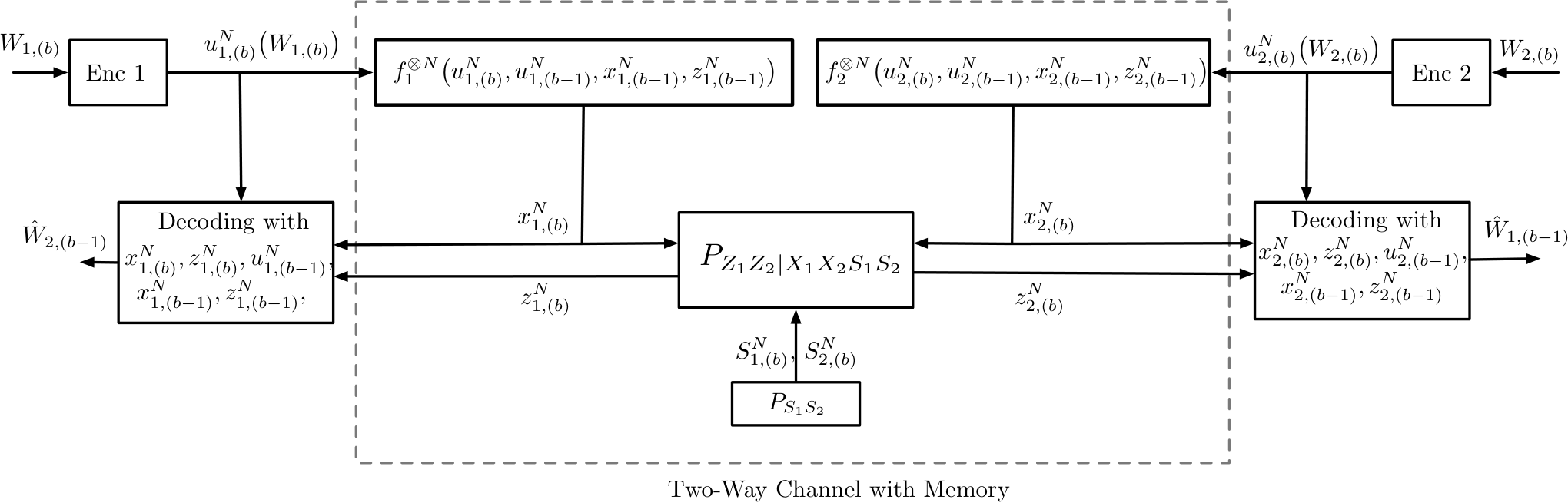
Fig. 7: Han’s coding scheme in a given block bb. Encoders transform the discrete-memoryless two-way channel into a channel with memory so as to be able to correlate the inputs of the two terminals. Encoding is then performed through the independent codewords u1,(b)Nu_{1,(b)}^{N} and u2,(b)Nu_{2,(b)}^{N}. Decoding of block-(b−1)(b-1) messages is performed based on the inputs/outputs in the two consecutive blocks b−1b-1 and bb.

The capacity region of the two-way channel, and thus the optimal coding scheme is still open for general channels. Various inner and outer bounds on the capacity region have been proposed. For example, Schalkwijk proposed an interesting inner bound for a binary multiplier channel based on a method that iteratively describes message points, an approach that is reminiscent of single-user feedback schemes. Han [29] and Kramer [30] proposed schemes that correlate the inputs of the two terminals in a block-fashion. While for Han’s coding scheme the correlation ensures a stationary distribution of the inputs and outputs across the blocks and thus still allows for single-letter rate-expressions, Kramer has to resort to multi-letter rate-expressions based on directed mutual informations. An interesting outer bound on the capacity region was proposed by Hekstra and Willems [22] again based on the dependence-balance idea, similar to the MAC with feedback.

The ISAC scheme we present in this manuscript is based on Han’s coding scheme, which is depicted in Figure 7 and described in the following. For convenience of notation, define

PZ1​Z2|X1​X2(z1,z2|x1,x2)=∑s1∈𝒮1,s2∈𝒮2PS1​S2(s1,s2)PZ1​Z2|X1​X2​S1​S2(z1,z2|x1,x2,s1,s2).P_{Z_{1}Z_{2}|X_{1}X_{2}}(z_{1},z_{2}|x_{1},x_{2})=\sum_{s_{1}\in\mathcal{S}_{1},s_{2}\in\mathcal{S}_{2}}P_{S_{1}S_{2}}(s_{1},s_{2})P_{Z_{1}Z_{2}|X_{1}X_{2}S_{1}S_{2}}(z_{1},z_{2}|x_{1},x_{2},s_{1},s_{2}). (36)

Han’s scheme splits the blocklength nn into B+1B+1 blocks of length N=n/(B+1)N=n/(B+1) each. Accordingly, throughout, we let X1,(b)N,X2,(b)N,S1,(b)N,S2,(b)N,Z1,(b)N,Z2,(b)NX_{1,(b)}^{N},X_{2,(b)}^{N},S_{1,(b)}^{N},S_{2,(b)}^{N},Z_{1,(b)}^{N},Z_{2,(b)}^{N} denote the block-bb inputs, states and outputs, e.g., S1,(b)N:=(S1​(b−1)​N+1,…,S1,b​N)S_{1,(b)}^{N}:=(S_{1(b-1)N+1},\ldots,S_{1,bN}). We also represent the two messages W1W_{1} and W2W_{2} in a one-to-one way as the BB-length tuples

Wk=(Wk,(1),…,Wk,(B)),k∈{1,2},W_{k}=(W_{k,(1)},\ldots,W_{k,(B)}),\qquad k\in\{1,2\}, (37)

where each Wk,(b)W_{k,(b)} is independent and uniformly distributed over [2N​R¯k]\left[2^{N\bar{R}_{k}}\right] for R¯k≜B+1B​Rk\bar{R}_{k}\triangleq\frac{B+1}{B}R_{k}.

Construct an independent code 𝒞k,(b)={uk,(b)N​(1),…,uk,(b)N​(2n​R¯k)}\mathcal{C}_{k,(b)}=\Big\{u_{k,(b)}^{N}(1),\ldots,u_{k,(b)}^{N}\big(2^{n\bar{R}_{k}}\big)\Big\} for each of the two terminals by picking entries i.i.d. according to some pmf PUkP_{U_{k}}. As shown in Figure 7, Terminal kk encodes Message Wk,(b)W_{k,(b)} by means of the codeword uk,(b)N​(Wk,(b))u_{k,(b)}^{N}(W_{k,(b)}) and sends the sequence

Xk,(b)N=fk⊗N​(uk,(b)N​(Wk,(b)),uk,(b−1)N​(Wk,(b−1)),xk,(b−1)N,zk,(b−1)N)X_{k,(b)}^{N}=f_{k}^{\otimes N}\left(u_{k,(b)}^{N}(W_{k,(b)}),\ u_{k,(b-1)}^{N}(W_{k,(b-1)}),\ x_{k,(b-1)}^{N},\ z_{k,(b-1)}^{N}\right) (38)

over the channel during block bb. Notice that by applying the function fkf_{k} to the block-bb codeword symbols as well as to the symbols of the block-(b−1)(b-1) codeword uk,(b−1)N​(Wk,(b−1))u_{k,(b-1)}^{N}(W_{k,(b-1)}) and the block-(b−1)(b-1) channel inputs and outputs xk,(b−1)Nx_{k,(b-1)}^{N} and zk,(b−1)Nz_{k,(b-1)}^{N}, the terminals introduce memory to the channel. An interesting point of view is to consider the transition of the codewords u1,(b)Nu_{1,(b)}^{N} and u2,(b)Nu_{2,(b)}^{N} to the channel outputs z1,(b)Nz_{1,(b)}^{N} and z2,(b)Nz_{2,(b)}^{N} as a virtual two-way channel with block-memory over which one can code and decode. Naturally, decoding of each message part Wk,(b)W_{k,(b)} is not based only on the signals in block (b)(b) because other blocks depend on this message as well. In Han’s scheme, decoding is over two consecutive blocks. Specifically, Terminal kk decodes the block-bb message Wk¯,(b)W_{\bar{k},(b)} using a joint-typicality decoder based on the block-bb inputs, outputs, and own transmitted codewords xk,(b)N,zk,(b)Nx_{k,(b)}^{N},z_{k,(b)}^{N} and uk,(b)Nu_{k,(b)}^{N}, as well as on the block-(b+1)(b+1) inputs and outputs xk,(b+1)Nx_{k,(b+1)}^{N} and zk,(b+1)Nz_{k,(b+1)}^{N}.

Notice that without any special care, the rate-region that is achievable with above scheme has to be described with a multi-letter expression because the joint pmf of the tuple x1,(b+1)N,z1,(b+1)N,u1,(b)N,x1,(b)N,z1,(b)Nx_{1,(b+1)}^{N},z_{1,(b+1)}^{N},u_{1,(b)}^{N},x_{1,(b)}^{N},z_{1,(b)}^{N} that Terminal 1 uses to decode codeword u2,(b)N​(Wk,(b))u_{2,(b)}^{N}(W_{k,(b)}) varies with the block bb. However, if one chooses a joint pmf PU1​U2​X1​X2​Z1​Z2P_{U_{1}U_{2}X_{1}X_{2}Z_{1}Z_{2}} satisfying the stationarity condition

PU1​U2​X1​X2​Z1​Z2​(u1,u2,x1,x2,z1,z2)\displaystyle P_{{U}_{1}{U}_{2}X_{1}X_{2}Z_{1}Z_{2}}(u_{1},u_{2},x_{1},x_{2},z_{1},z_{2}) (39)
=\displaystyle= ∑u~1,u~2,x~1,x~2,z~1,z~2PZ1​Z2|X1​X2(z1,z2|x1,x2)𝟙{x1=f1(u1,u~1,x~1,z~1)}\displaystyle\sum_{\tilde{u}_{1},\tilde{u}_{2},\tilde{x}_{1},\tilde{x}_{2},\tilde{z}_{1},\tilde{z}_{2}}P_{Z_{1}Z_{2}|X_{1}X_{2}}(z_{1},z_{2}|x_{1},x_{2})\mathbbm{1}\{x_{1}=f_{1}(u_{1},\tilde{u}_{1},\tilde{x}_{1},\tilde{z}_{1})\}
𝟙{x2=f2(u2,u~2,x~2,z~2)}⋅PU1(u1)PU2(u2)PU1​U2​X1​X2​Z1​Z2(u~1,u~2,x~1,x~2,z~1,z~2),\displaystyle\mathbbm{1}\{x_{2}=f_{2}(u_{2},\tilde{u}_{2},\tilde{x}_{2},\tilde{z}_{2})\}\cdot P_{U_{1}}(u_{1})P_{U_{2}}(u_{2})P_{{U}_{1}{U}_{2}{X}_{1}{X}_{2}Z_{1}Z_{2}}(\tilde{u}_{1},\tilde{u}_{2},\tilde{x}_{1},\tilde{x}_{2},\tilde{z}_{1},\tilde{z}_{2}),

where PU1P_{U_{1}} and PU2P_{U_{2}} are the marginals of PU1​U2​X1​X2​Z1​Z2P_{U_{1}U_{2}X_{1}X_{2}Z_{1}Z_{2}}, then the pmf of the tuple of sequences x1,(b+1)N,xN2,(b+1),z1,(b+1)N,z2,(b+1)N,u1,(b)N,u2,(b)N,x1,(b)N,x2,(b)N,z1,(b)N,z2,(b)Nx_{1,(b+1)}^{N},x{{}^{N}}_{2,(b+1)},z_{1,(b+1)}^{N},z_{2,(b+1)}^{N},u_{1,(b)}^{N},u_{2,(b)}^{N},x_{1,(b)}^{N},x_{2,(b)}^{N},z_{1,(b)}^{N},z_{2,(b)}^{N} is independent of the block index bb. This allows to characterize the rate region achieved by the described coding scheme using a single-letter expression. All rate-pairs (R1,R2)(R_{1},R_{2}) are achievable that satisfy

R1\displaystyle R_{1} ≤\displaystyle\leq I⁡(U1,X2,Z2,U~2,X~2,Z~2)\displaystyle I(U_{1};X_{2},Z_{2},\tilde{U}_{2},\tilde{X}_{2},\tilde{Z}_{2}) (40a)
R2\displaystyle R_{2} ≤\displaystyle\leq I⁡(U2,X1,Z1,U~1,X~1,Z~1),\displaystyle I(U_{2};X_{1},Z_{1},\tilde{U}_{1},\tilde{X}_{1},\tilde{Z}_{1}), (40b)

where (U1,U2,X1,X2,Z1,Z2,U~1,U~2,X~1,X~2,Z~1,Z~2)(U_{1},U_{2},X_{1},X_{2},Z_{1},Z_{2},\tilde{U}_{1},\tilde{U}_{2},\tilde{X}_{1},\tilde{X}_{2},\tilde{Z}_{1},\tilde{Z}_{2}) are distributed according to the pmf

PU1​U2​X1​X2​Z1​Z2​U~1​U~2​X~1​X~2​Z~1​Z~2​(u1,u2,x1,x2,z1,z2,u~1,u~2,x~1,x~2,z~1,z~2)\displaystyle P_{U_{1}U_{2}X_{1}X_{2}Z_{1}Z_{2}\tilde{U}_{1}\tilde{U}_{2}\tilde{X}_{1}\tilde{X}_{2}\tilde{Z}_{1}\tilde{Z}_{2}}(u_{1},u_{2},x_{1},x_{2},z_{1},z_{2},\tilde{u}_{1},\tilde{u}_{2},\tilde{x}_{1},\tilde{x}_{2},\tilde{z}_{1},\tilde{z}_{2}) (41)
=\displaystyle= PZ1​Z2|X1​X2(z1,z2|x1,x2)𝟙{x1=f1(u1,u~1,x~1,z~1)}𝟙{x2=f2(u2,u~2,x~2,z~2)}\displaystyle P_{Z_{1}Z_{2}|X_{1}X_{2}}(z_{1},z_{2}|x_{1},x_{2})\mathbbm{1}\{x_{1}=f_{1}(u_{1},\tilde{u}_{1},\tilde{x}_{1},\tilde{z}_{1})\}\mathbbm{1}\{x_{2}=f_{2}(u_{2},\tilde{u}_{2},\tilde{x}_{2},\tilde{z}_{2})\}
⋅PU1​(u1)​PU2​(u2)​PU1​U2​X1​X2​Z1​Z2​(u~1,u~2,x~1,x~2,z~1,z~2).\displaystyle\cdot P_{U_{1}}(u_{1})P_{U_{2}}(u_{2})P_{{U}_{1}{U}_{2}{X}_{1}{X}_{2}Z_{1}Z_{2}}(\tilde{u}_{1},\tilde{u}_{2},\tilde{x}_{1},\tilde{x}_{2},\tilde{z}_{1},\tilde{z}_{2}).

This recovers Han’s theorem:

Theorem 4 (Han’s Achievable Region for Two-Way Channels [29]).

Any nonnegative rate-pair (R1,R2)(R_{1},R_{2}) is achievable over the two-way channel if it satisfies Inequalities (40) for some choice of pmf PU1​U2​X1​X2​Z1​Z2P_{U_{1}U_{2}X_{1}X_{2}Z_{1}Z_{2}} and functions f1f_{1} and f2f_{2} satisfying the stationarity condition (39).

For certain cases the above theorem can be simplified, and for certain channels the simplified region even coincides with capacity. The simplification is obtained by choosing the two functions f1f_{1} and f2f_{2} to simply produce the codewords u1,(b−1)Nu_{1,(b-1)}^{N} and u2,(b−1)Nu_{2,(b-1)}^{N} from the previous block33 3 The delay of a block introduced in this scheme is not crucial, it simply comes from the fact that Han’s scheme decodes the block-(b−1)(b-1) codewords based on the block-bb outputs. In this special case without adaptation, Han’s scheme could be simplified by transmitting and decoding the codewords u1,(b−1)Nu_{1,(b-1)}^{N} and u2,(b−1)Nu_{2,(b-1)}^{N} directly in block b−1b-1 without further delay. and ignore the other arguments. In this case, the set of rates that can be achieved coincides with the following inner bound that was first proposed by Shannon [31].

Theorem 5 (Shannon’s Inner Bound, [31]).

A pair of nonnegative pairs (R1,R2)(R_{1},R_{2}) is achievable if it satisfies

R1≤I⁡(X1;Z2|X2)\displaystyle R_{1}\leq I(X_{1};Z_{2}|X_{2}) (42a)
R2≤I⁡(X2;Z1|X1),\displaystyle R_{2}\leq I(X_{2};Z_{1}|{\color[rgb]{0,0,0}X_{1}}), (42b)

for some input pmfs PX1P_{X_{1}} and PX2P_{X_{2}} and where (X1,X2,Z1,Z2)∼PX1​PX2​PZ1​Z2|X1​X2(X_{1},X_{2},Z_{1},Z_{2})\sim P_{X_{1}}P_{X_{2}}P_{Z_{1}Z_{2}|X_{1}X_{2}}.

V-B Collaborative Sensing and Communication based on Han’s Two-Way Coding Scheme

We extend Han’s coding scheme to include also collaborative sensing, that means each terminal compresses its block-bb inputs and outputs so as to capture information about the other terminal’s state and sends this state-information in the next-following block. In this first collaborative sensing and communication scheme that we present here, the sensing (compression) does not affect the communication (except possibly for the choice of the pmf PU1​U2​X1​X2​Z1​Z2P_{U_{1}U_{2}X_{1}X_{2}Z_{1}Z_{2}}).

Refer to caption
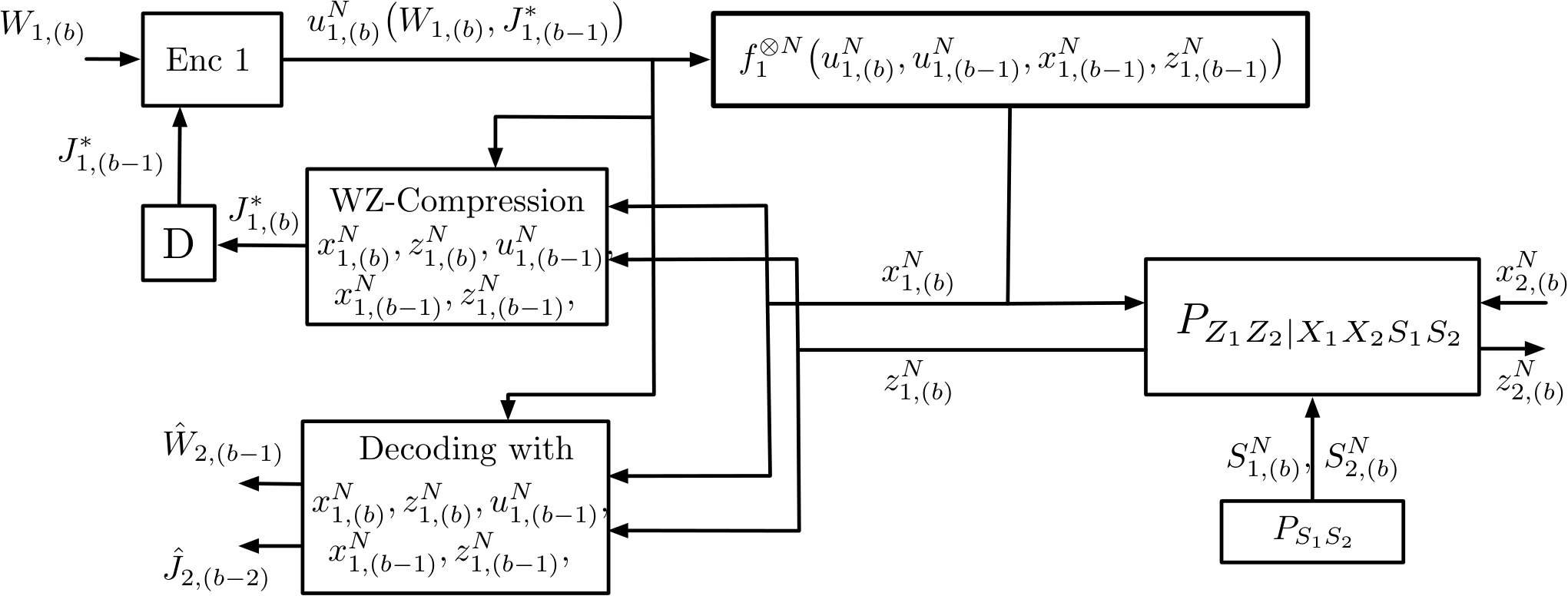
Fig. 8: A first collaborative-sensing version of Han’s coding scheme. The figure illustrates the encoding and decoding operations in a given block bb at Terminal 1; Terminal 2 behaves analogously. To facilitate sensing at Terminal 2, Terminal 1 compresses its block-bb channel inputs and outputs, together with its inputs, outputs, and codeword from the previous block (b−1)(b-1) (which are all resent in block bb) using Wyner-Ziv compression [32] to account for the side-information at Terminal 2.

In fact, we again use Han’s encodings and decodings as described in the previous subsection, except that the block-bb codeword not only encodes message Wk,(b)W_{k,(b)} but also a compression index Jk,(b−1)∗J_{k,(b-1)}^{*} that carries information about the block-(b−1)(b-1) state Sk¯,(b−1)S_{\bar{k},(b-1)}. This compression index is then decoded at Terminal k¯\bar{k} after block (b+1)(b+1) simultaneously with message Wk,(b)W_{k,(b)}. See Figure 8.

The analysis of the communication-part of our ISAC scheme is similar as in Han’s scheme. Since the compression indices take parts of the place reserved for ordinary messages in Han’s scheme, their rates RWZ,1R_{\textnormal{WZ},1} and RWZ,2R_{\textnormal{WZ},2} have to be subtracted from Han’s communication rates. We thus have the following constraints for reliable communication and reliable decoding of the compression indices:

R1+RWZ,1\displaystyle R_{1}+R_{\textnormal{WZ},1} ≤\displaystyle\leq I⁡(U1,X2,Z2,U~2,X~2,Z~2)\displaystyle I(U_{1};X_{2},Z_{2},\tilde{U}_{2},\tilde{X}_{2},\tilde{Z}_{2}) (43a)
R2+RWZ,2\displaystyle R_{2}+R_{\textnormal{WZ},2} ≤\displaystyle\leq I⁡(U2,X1,Z1,U~1,X~1,Z~1).\displaystyle I(U_{2};X_{1},Z_{1},\tilde{U}_{1},\tilde{X}_{1},\tilde{Z}_{1}). (43b)

It remains to explain the compression and state estimation in more details. In our scheme, the index Jk,(b−1)∗J_{k,(b-1)}^{*} is obtained by means of a Wyner-Ziv compression [32] that lossily compresses the tuple (xk,(b−1)N,zk,(b−1)N,uk,(b−2)N,xk,(b−2)N,zk,(b−2)N)(x_{k,(b-1)}^{N},z_{k,(b-1)}^{N},u_{k,(b-2)}^{N},x_{k,(b-2)}^{N},z_{k,(b-2)}^{N}) for a decoder that has side-information (xk¯,(b−1)N,zk¯,(b−1)N,uk¯,(b−2)N,xk¯,(b−2)N,zk¯,(b−2)N)(x_{\bar{k},(b-1)}^{N},z_{\bar{k},(b-1)}^{N},u_{\bar{k},(b-2)}^{N},x_{\bar{k},(b-2)}^{N},z_{\bar{k},(b-2)}^{N}). In order for the decoder to be able to correctly reconstruct the compression codeword, the Wyner-Ziv codes need to be of rates at least [32]

RWZ,k>I(Vk;Xk,Zk,U~k,X~k,Z~k|Xk¯,Zk¯,U~k¯,X~k¯,Z~k¯),k∈{1,2},\displaystyle R_{\textnormal{WZ},k}>I(V_{k};X_{k},Z_{k},\tilde{U}_{k},\tilde{X}_{k},\tilde{Z}_{k}|X_{\bar{k}},Z_{\bar{k}},\tilde{U}_{\bar{k}},\tilde{X}_{\bar{k}},\tilde{Z}_{\bar{k}}),\qquad k\in\{1,2\}, (44)

where the tuple (U1,U2,X1,X2,Z1,Z2,U~1,U~2,X~1,X~2,Z~1,Z~2)(U_{1},U_{2},X_{1},X_{2},Z_{1},Z_{2},\tilde{U}_{1},\tilde{U}_{2},\tilde{X}_{1},\tilde{X}_{2},\tilde{Z}_{1},\tilde{Z}_{2}) refers to the auxiliary random variables chosen by Han’s scheme of joint pmf as in (41) and V1V_{1} and V2V_{2} can be any random variables satisfying the Markov chains:

Vk→(Xk,Zk,U~k,X~k,Z~k)→(Xk¯,Zk¯,U~k¯,X~k¯,Z~k¯,Sk,Sk¯).\displaystyle V_{k}\to(X_{k},Z_{k},\tilde{U}_{k},\tilde{X}_{k},\tilde{Z}_{k})\to(X_{\bar{k}},Z_{\bar{k}},\tilde{U}_{\bar{k}},\tilde{X}_{\bar{k}},\tilde{Z}_{\bar{k}},S_{k},S_{\bar{k}}). (45)

In Wyner-Ziv coding, the encoder produces a codeword that is then reconstructed also at the receiver. We shall denote these codewords by vk,(b−1)N​(Jk,(b−1)∗,ℓk,(b−1))v_{k,(b-1)}^{N}(J_{k,(b-1)}^{*},\ell_{k,(b-1)}), for k∈{1,2}k\in\{1,2\}, where ℓk,(b−1)\ell_{k,(b-1)} denotes a binning-index that does not have to be conveyed to the Terminal k¯\bar{k} because this latter can recover it from its side-information. Thus, after block (b+1)(b+1) and after decoding index Jk,(b−1)∗J_{{k},(b-1)}^{*}, with high probability Terminal k¯\bar{k} can reconstruct the codeword vk,(b−1)N​(Jk,(b−1)∗,ℓk,(b−1))v_{{k},(b-1)}^{N}(J_{k,(b-1)}^{*},\ell_{k,(b-1)}) chosen at Terminal kk.

Terminal kk can wait arbitrarily long to produce an estimate of the state-sequence SkNS_{k}^{N}. We propose that it waits after the block-(b+1)(b+1) decoding to reconstruct the block-bb state Sk,(b)NS_{k,(b)}^{N} by applying an optimal symbol-by-symbol estimator to the related sequences of inputs, outputs, and channel codewords of blocks b−1b-1 and bb, as well as on the compression codeword vk¯,(b)Nv_{\bar{k},(b)}^{N}:

S^k,(b)N=ϕ~2,k∗⊗N(vk¯,(b)N,xk,(b)N,zk,(b)N,u^k¯,(b),uk,(b−1)N,xk,(b−1)N,zk,(b−1)N,u^k¯,(b−1)),\hat{S}^{N}_{k,(b)}=\tilde{\phi}_{2,k}^{*\otimes N}\left(v_{\bar{k},(b)}^{N},x_{k,(b)}^{N},z_{k,(b)}^{N},\hat{u}_{\bar{k},(b)},u_{k,(b-1)}^{N},x_{k,(b-1)}^{N},z_{k,(b-1)}^{N},\hat{u}_{\bar{k},(b-1)}\right), (46)

where

ϕ~2,k∗​(vk¯,xk,zk,uk¯,u~k,x~k,z~k,u~k¯):=arg​min⁡∑sk∈𝒮ksk′∈𝒮k^⁡PSk|Xk​Zk​Uk¯​(sk|xk,zk,uk¯)​dk​(sk,sk′).\displaystyle\tilde{\phi}_{2,k}^{*}(v_{\bar{k}},x_{k},z_{k},u_{\bar{k}},\tilde{u}_{k},\tilde{x}_{k},\tilde{z}_{k},\tilde{u}_{\bar{k}}):=\textnormal{arg}\min_{s_{k}^{\prime}\in\hat{\mathcal{S}_{k}}}\sum_{s_{k}\in\mathcal{S}_{k}}P_{S_{k}|X_{k}Z_{k}U_{\bar{k}}}(s_{k}|x_{k},z_{k},u_{\bar{k}})\;d_{k}(s_{k},s_{k}^{\prime}). (47)

By (43) and (44) and standard typicality arguments, one obtains the following theorem. (The theorem is a special case of the next-following theorem, for which we provide a detailed analysis in the extended version [33].)

Theorem 6 (Inner Bound via Separate Source-Channel Coding).

Any nonnegative rate-distortion quadruple (R1,R2,D1,D2)(R_{1},R_{2},D_{1},D_{2}) is achievable if it satisfies the following two rate-constraints

R1\displaystyle R_{1} ≤\displaystyle\leq I(U1;X2,Z2,U~2,X~2,Z~2)−I(V1;X1,Z1,U~1,X~1,Z~1|X2,Z2,U~2,X~2,Z~2)\displaystyle I(U_{1};X_{2},Z_{2},\tilde{U}_{2},\tilde{X}_{2},\tilde{Z}_{2})-I(V_{1};X_{1},Z_{1},\tilde{U}_{1},\tilde{X}_{1},\tilde{Z}_{1}|X_{2},Z_{2},\tilde{U}_{2},\tilde{X}_{2},\tilde{Z}_{2}) (48a)
R2\displaystyle R_{2} ≤\displaystyle\leq I(U2;X1,Z1,U~1,X~1,Z~1)−I(V2;X2,Z2,U~2,X~2,Z~2|X1,Z1,U~1,X~1,Z~1),\displaystyle I(U_{2};X_{1},Z_{1},\tilde{U}_{1},\tilde{X}_{1},\tilde{Z}_{1})-I(V_{2};X_{2},Z_{2},\tilde{U}_{2},\tilde{X}_{2},\tilde{Z}_{2}|X_{1},Z_{1},\tilde{U}_{1},\tilde{X}_{1},\tilde{Z}_{1}), (48b)
and the two distortion constraints
E​[d1​(S1,ϕ~2,1∗​(V2,X1,Z1,U2,U~1,X~1,Z~1,U~2))]\displaystyle\textnormal{{E}}\!\left[d_{1}\big(S_{1},\ \tilde{\phi}_{2,1}^{*}(V_{2},X_{1},Z_{1},U_{2},\tilde{U}_{1},\tilde{X}_{1},\tilde{Z}_{1},\tilde{U}_{2})\big)\right] ≤\displaystyle\leq D1\displaystyle D_{1} (48c)
E​[d2​(S2,ϕ~2,2∗​(V1,X2,Z2,U1,U~2,X~2,Z~2,U~2))]\displaystyle\textnormal{{E}}\!\left[d_{2}\big(S_{2},\ \tilde{\phi}_{2,2}^{*}(V_{1},X_{2},Z_{2},U_{1},\tilde{U}_{2},\tilde{X}_{2},\tilde{Z}_{2},\tilde{U}_{2})\big)\right] ≤\displaystyle\leq D2\displaystyle D_{2} (48d)

for some choice of pmf PU1​U2​X1​X2​Z1​Z2P_{U_{1}U_{2}X_{1}X_{2}Z_{1}Z_{2}} and functions f1f_{1} and f2f_{2} satisfying the stationarity condition (39) and V1,V2V_{1},V_{2} satisfying the Markov chains (45).

Similarly to Shannon’s inner bound, we can obtain the following corollary by setting Xk=U~kX_{k}=\tilde{U}_{k}.

Corollary 1 (Inner Bound via Non-Adaptive Coding).

Any nonnegative rate-distortion quadruple (R1,R2,D1,D2)(R_{1},R_{2},D_{1},D_{2}) is achievable if it satisfies the following two rate-constraints

R1\displaystyle R_{1} ≤\displaystyle\leq I(X1;X2,Z2)−I(V1;X1,Z1|X2,Z2)\displaystyle I(X_{1};X_{2},Z_{2})-I(V_{1};X_{1},Z_{1}|X_{2},Z_{2}) (49a)
R2\displaystyle R_{2} ≤\displaystyle\leq I(X2;X1,Z1)−I(V2;X2,Z2|X1,Z1),\displaystyle I(X_{2};X_{1},Z_{1})-I(V_{2};X_{2},Z_{2}|X_{1},Z_{1}), (49b)
and the two distortion constraints
E​[d1​(S1,ϕ~2,1∗​(V2,X1,X2,Z1))]\displaystyle\textnormal{{E}}\!\left[d_{1}\big(S_{1},\ \tilde{\phi}_{2,1}^{*}(V_{2},X_{1},X_{2},Z_{1})\big)\right] ≤\displaystyle\leq D1\displaystyle D_{1} (49c)
E​[d2​(S2,ϕ~2,2∗​(V1,X1,X2,Z2))]\displaystyle\textnormal{{E}}\!\left[d_{2}\big(S_{2},\ \tilde{\phi}_{2,2}^{*}(V_{1},X_{1},X_{2},Z_{2})\big)\right] ≤\displaystyle\leq D2\displaystyle D_{2} (49d)

for some choice of pmfs PX1P_{X_{1}}, PX2P_{X_{2}}, PV1|X1,Z1P_{V_{1}|X_{1},Z_{1}}, and PV2|X2,Z2P_{V_{2}|X_{2},Z_{2}}.

As the following example shows, above corollary achieves the fundamental rate-distortion tradeoff for some channels.

Example 3.

Consider the following state-dependent two-way channel

Z1\displaystyle Z_{1} =\displaystyle= X1⊕X2⊕S2andZ2=X1⊕X2⊕S1,\displaystyle X_{1}\oplus X_{2}\oplus S_{2}\qquad\textnormal{and}\qquad Z_{2}=X_{1}\oplus X_{2}\oplus S_{1}, (50a)

where inputs, outputs, and states are binary and S1S_{1} and S2S_{2} are independent Bernoulli-p1p_{1} and p2p_{2} random variables, for p1,p2∈[0,1/2]p_{1},p_{2}\in[0,1/2]. Notice that Terminal 1’s outputs depend on the state desired at Terminal 2 and Terminal 2’s outputs on the state desired at Terminal 1, which calls for collaborative sensing.

Whenever Dk¯<pk¯D_{\bar{k}}<p_{\bar{k}}, we chooose

Vk\displaystyle V_{k} =\displaystyle= Zk⊕Xk⊕Bk=Xk¯⊕Sk¯⊕Bk\displaystyle Z_{k}\oplus X_{k}\oplus B_{k}=X_{\bar{k}}\oplus S_{\bar{k}}\oplus B_{k} (51)

where BkB_{k} is an independent Bernoulli-DkD_{k} random variable. If Dk≥pkD_{k}\geq p_{k}, choose VkV_{k} a constant. Inputs X1X_{1} and X2X_{2} are chosen independent Bernoulli-1/21/2, i.e., capacity-achieving on channels with Bernoulli-noses. When Dk¯<pk¯D_{\bar{k}}<p_{\bar{k}}, the optimal symbo-by-symbol state-estimator is

ϕ~2,k¯∗​(vk,x1,x2,zk¯)=vk⊕xk¯\tilde{\phi}_{2,{\bar{k}}}^{*}(v_{k},x_{1},x_{2},z_{\bar{k}})=v_{k}\oplus x_{\bar{k}} (52)

and otherwise it is the constant estimator ϕ~2,k¯∗​(vk,x1,x2,zk¯)=0\tilde{\phi}_{2,{\bar{k}}}^{*}(v_{k},x_{1},x_{2},z_{\bar{k}})=0.

For the described choice of random variables, Corollary 1 evaluates to the set of rate-distortion tuples (R1,R2,D1,D2)(R_{1},R_{2},D_{1},D_{2}) satisfying

Rk\displaystyle R_{k} ≤\displaystyle\leq 1−Hb​(pk)−max⁡{0,Hb​(pk¯)−Hb​(Dk¯)},k∈{1,2},\displaystyle 1-H_{\text{b}}(p_{k})-\max\{0,\ H_{\text{b}}(p_{\bar{k}})-H_{\text{b}}(D_{\bar{k}})\},\qquad k\in\{1,2\}, (53)

and achieves the fundamental rate-distortion region as we show through a converse in Appendix A. The region in (53) is concave (because the rate-distortion function max⁡{0,Hb​(pk¯)−Hb​(Dk¯)}\max\{0,\ H_{\text{b}}(p_{\bar{k}})-H_{\text{b}}(D_{\bar{k}})\} is convex), and thus improves over classic time- and resource-sharing schemes. It also improves over a similar ISAC scheme without collaborative sensing where the compression codewords V1V_{1} and V2V_{2} are set to constants. In this latter case, only rate-distortion tuples are possible that satisfy Dk≥pkD_{k}\geq p_{k}, for k∈{1,2}k\in\{1,2\}.

Remark 6.

For certain channels and state-distributions Theorem 6 can be improved with the idea of coded time-sharing. The same applies for Theorem 7 in the next-following section.

V-C Collaborative Sensing and JSCC Scheme

In this scheme, we fully integrate the compression into the communication scheme, in a similar way that hybrid coding [34] uses a single codeword for compression and channel coding in source-channel coding applications.

Refer to caption
Fig. 9: A ISAC scheme integrating collaborative sensing for D2D into Han’s two-way coding scheme by means of hybrid coding. A single codeword is used both for compression and for channel coding.

Encoding and decoding in block bb of the new scheme are depicted in Figure 9. The main difference compared to the scheme in the previous subsection is that here the block-bb codeword u1,(b)Nu_{1,(b)}^{N} is correlated with the inputs and outputs in the previous block (b−1)(b-1).44 4 In the previous scheme, the compression codeword v1,(b)Nv_{1,(b)}^{N} was correlated with the block-(b−1)(b-1) signals but not the channel coding codeword u1,(b)Nu^{N}_{1,(b)}. Now the codeword u1,(b)Nu_{1,(b)}^{N} acts both as a compression codeword and as a channel coding codeword. This correlation introduces additional dependence between blocks, which was previously missing because of the independence of the compression codewords and the codewords used for channel coding in the next block. To still obtain a stationary distribution on the codewords and channel inputs/outputs, which then allows for a single-letter characterization of the performance of the scheme, one has to choose a joint pmf PU1′​U2′​Z1​Z2​X1​X2​U1​U2P_{U_{1}^{\prime}U_{2}^{\prime}Z_{1}Z_{2}X_{1}X_{2}U_{1}U_{2}}, conditional pmfs PU1′|X1​Z1​U~1​X~1​Z~1P_{U_{1}^{\prime}|X_{1}Z_{1}\tilde{U}_{1}\tilde{X}_{1}\tilde{Z}_{1}} and PU2′|X2​Z2​U~2​X~2​Z~2P_{U_{2}^{\prime}|X_{2}Z_{2}\tilde{U}_{2}\tilde{X}_{2}\tilde{Z}_{2}} as well as functions f1f_{1} and f2f_{2} on appropriate domains satisfying the new stationarity condition

PU1′​U2′​Z1​Z2​X1​X2​U1​U2​(u1′,u2′,z1,z2,x1,x2)\displaystyle P_{U_{1}^{\prime}U_{2}^{\prime}Z_{1}Z_{2}X_{1}X_{2}U_{1}U_{2}}(u_{1}^{\prime},u_{2}^{\prime},z_{1},z_{2},x_{1},x_{2}) (54)
=\displaystyle= ∑u~1,u~2,x~1,x~2,z~1,z~2PU1′|X1​Z1​U~1​X~1​Z~1​(u1′|u1,x1,z1,u~1,x~1,z~1)​PU2′|X2​Z2​U~2​X~2​Z~2​(u2′|x2,z2,u2,u~2,x~2,z~2)\displaystyle\sum_{\tilde{u}_{1},\tilde{u}_{2},\tilde{x}_{1},\tilde{x}_{2},\tilde{z}_{1},\tilde{z}_{2}}P_{U_{1}^{\prime}|X_{1}Z_{1}\tilde{U}_{1}\tilde{X}_{1}\tilde{Z}_{1}}(u_{1}^{\prime}|u_{1},x_{1},z_{1},\tilde{u}_{1},\tilde{x}_{1},\tilde{z}_{1})P_{U_{2}^{\prime}|X_{2}Z_{2}\tilde{U}_{2}\tilde{X}_{2}\tilde{Z}_{2}}(u_{2}^{\prime}|x_{2},z_{2},u_{2},\tilde{u}_{2},\tilde{x}_{2},\tilde{z}_{2})
⋅PZ1​Z2|X1​X2(z1,z2|x1,x2)𝟙{x1=f1(u1,u~1,x~1,z~1)}𝟙{x2=f2(u2,u~2,x~2,z~2)}\displaystyle\hskip 56.9055pt\cdot P_{Z_{1}Z_{2}|X_{1}X_{2}}(z_{1},z_{2}|x_{1},x_{2})\mathbbm{1}\{x_{1}=f_{1}(u_{1},\tilde{u}_{1},\tilde{x}_{1},\tilde{z}_{1})\}\mathbbm{1}\{x_{2}=f_{2}(u_{2},\tilde{u}_{2},\tilde{x}_{2},\tilde{z}_{2})\}
⋅PU1′​U2′​Z1​Z2​X1​X2​U1​U2​(u1,u2,z~1,z~2,x~1,x~2,u~1,u~2),\displaystyle\hskip 113.81102pt\cdot P_{U_{1}^{\prime}U_{2}^{\prime}Z_{1}{Z}_{2}{X}_{1}X_{2}{U}_{1}{U}_{2}}(u_{1},u_{2},\tilde{z}_{1},\tilde{z}_{2},\tilde{x}_{1},\tilde{x}_{2},\tilde{u}_{1},\tilde{u}_{2}),

In the following, all mentioned conditional and marginal pmfs are with respect to the joint pmf PU1′​U2′​Z1​Z2​X1​X2​U1​U2​U~1​U~2​W~1​W~2​V~1​V~2P_{U_{1}^{\prime}U_{2}^{\prime}Z_{1}Z_{2}X_{1}X_{2}U_{1}U_{2}\tilde{U}_{1}\tilde{U}_{2}\tilde{W}_{1}\tilde{W}_{2}\tilde{V}_{1}\tilde{V}_{2}} indicated by the summand in (54).

We next explain the code construction, encodings and decodings.

For each k∈{1,2}k\in\{1,2\}, for each block b∈{1,…,B+1}b\in\{1,\ldots,B+1\}, and each message mk∈[2N​R¯k]m_{k}\in[2^{N\bar{R}_{k}}], choose a subcodebook {uk,(b)N​(mk,j):j∈[2N​Rk′]}\{u_{k,(b)}^{N}(m_{k},j)\colon j\in[2^{NR_{k}^{\prime}}]\} by picking all entries i.i.d. PUk′P_{U_{k}^{\prime}}. Terminal kk then picks the codeword uk,(b)N​(Wk,(b),j)u_{k,(b)}^{N}(W_{k,(b)},j) so that the following joint-typicality check is satisfied for some fixed ϵ>0\epsilon>0:

(uk,(b)N​(Wk,(b),j),xk,(b−1)N,zk,(b−1)N,uk,(b−2)N,xk,(b−2)N,zk,(b−2)N)∈𝒯ϵN​(PUk′​Xk​Zk​U~k​X~k​Z~k),\displaystyle\big(u_{k,(b)}^{N}(W_{k,(b)},j),x_{k,(b-1)}^{N},\,z_{k,(b-1)}^{N},\,u_{k,(b-2)}^{N},\,x_{k,(b-2)}^{N},\,z_{k,(b-2)}^{N}\big)\in\mathcal{T}_{\epsilon}^{N}\Big(P_{U_{k}^{\prime}X_{k}Z_{k}\tilde{U}_{k}\tilde{X}_{k}\tilde{Z}_{k}}\Big), (55)

and sets Jk,(b−1)∗=jJ_{k,(b-1)}^{*}=j. By standard arguments, such an index jj exists with probability tending to 1 as N→∞N\to\infty if

Rk′\displaystyle{R}_{k}^{\prime} ≥\displaystyle\geq I⁡(Uk′,Xk,Zk,U~k,X~k,Z~k),k∈{1,2}.\displaystyle I(U_{k}^{\prime};X_{k},Z_{k},\tilde{U}_{k},\tilde{X}_{k},\tilde{Z}_{k}),\quad k\in\{1,2\}. (56)

Terminal kk then sends the block-bb input sequence

Xk,(b)N=fk⊗N​(uk,(b)N​(Wk,(b)​Jk,(b−1)∗),uk,(b−1)N,xk,(b−1)n,zk,(b−1)N).X_{k,(b)}^{N}=f_{k}^{\otimes N}\left(u_{k,(b)}^{N}\big(W_{k,(b)}J_{k,(b-1)}^{*}\big),u_{k,(b-1)}^{N},x_{k,(b-1)}^{n},z_{k,(b-1)}^{N}\right). (57)

Decoding is again performed using a joint-typicality decoder. At the end of block bb, Terminal kk looks for indices w^k¯\hat{w}_{\bar{k}} and j^k¯\hat{j}_{\bar{k}} satisfying the two typicality checks

(uk¯,(b−1)N​(w^k¯,j^k¯),xk,(b)N,zk,(b)N,uk,(b−1)N​xk,(b−1)N,zk,(b−1)N)∈𝒯ϵN​(PU~k¯​Xk​Zk​U~k​X~k​Z~k)\displaystyle\big(u_{\bar{k},(b-1)}^{N}(\hat{w}_{\bar{k}},\hat{j}_{\bar{k}}),x_{k,(b)}^{N},\,z_{k,(b)}^{N},\,u_{k,(b-1)}^{N}\,x_{k,(b-1)}^{N},\,z_{k,(b-1)}^{N}\big)\in\mathcal{T}_{\epsilon}^{N}\Big(P_{\tilde{U}_{\bar{k}}X_{k}Z_{k}\tilde{U}_{k}\tilde{X}_{k}\tilde{Z}_{k}}\Big) (58)

and

(uk¯,(b−1)N​(w^k¯,j^k¯),xk,(b−2)N,zk,(b−2)N,uk,(b−3)n,xk,(b−3)N,zk,(b−3)N)∈𝒯ϵN​(PUk¯​Xk​Zk​U~k​X~k​Z~k).\displaystyle\big(u_{\bar{k},(b-1)}^{N}(\hat{w}_{\bar{k}},\hat{j}_{\bar{k}}),x_{k,(b-2)}^{N},\,z_{k,(b-2)}^{N},\,u_{k,(b-3)}^{n},\,x_{k,(b-3)}^{N},\,z_{k,(b-3)}^{N}\big)\in\mathcal{T}_{\epsilon}^{N}\left(P_{U_{\bar{k}}X_{k}Z_{k}\tilde{U}_{k}\tilde{X}_{k}\tilde{Z}_{k}}\right). (59)

If a unique pair of such element exists, set W^k¯,(b−1)=wk¯\hat{W}_{\bar{k},(b-1)}=w_{\bar{k}} and u^k¯,(b−1)N≜uk¯,(b−1)N​(w^k¯,j^k¯)\hat{u}_{\bar{k},(b-1)}^{N}\triangleq u_{\bar{k},(b-1)}^{N}(\hat{w}_{\bar{k}},\hat{j}_{\bar{k}}). Decoding is successful with probability tending to 0 as N→∞N\to\infty if

R¯k¯+Rk¯′\displaystyle\bar{R}_{\bar{k}}+{R}_{\bar{k}}^{\prime} ≤\displaystyle\leq I⁡(U~k¯,Xk,Zk,U~k,X~k,Z~k)+I⁡(Uk¯,Xk,Zk,U~k,X~k,Z~k),k∈{1,2}.\displaystyle I(\tilde{U}_{\bar{k}};X_{k},Z_{k},\tilde{U}_{k},\tilde{X}_{k},\tilde{Z}_{k})+I(U_{\bar{k}};X_{k},Z_{k},\tilde{U}_{k},\tilde{X}_{k},\tilde{Z}_{k}),\quad k\in\{1,2\}. (60)

State-estimation is similar to (46), but where Terminal kk replaces the compression codeword vk,(b)Nv_{k,(b)}^{N} by the joint source-channel codeword uk,(b+1)Nu_{k,(b+1)}^{N} and similarly to hybrid coding also uses the inputs/outputs corresponding to the block where the codeword u1,(b+1)Nu_{1,(b+1)}^{N} is sent, i.e., inputs and outputs in block b+1b+1. Thus, Terminal kk computes its estimate of the block-bb state as:

s^k,(b)N=ϕ2,k∗⊗N(u^k¯,(b+1)N,xk,(b+1)N,zk,(b+1)N,u^k¯,(b)N,xk,(b)N,zk,(b)N,uk,(b−1)N,xk,(b−1)N,zk,(b−1)N,u^k¯,(b−1)N),\hat{s}^{N}_{k,(b)}=\phi_{2,k}^{*\otimes N}\big(\hat{u}_{\bar{k},(b+1)}^{N},x_{k,(b+1)}^{N},z_{k,(b+1)}^{N},\hat{u}_{\bar{k},(b)}^{N},x_{k,(b)}^{N},z_{k,(b)}^{N},u_{k,(b-1)}^{N},x_{k,(b-1)}^{N},z_{k,(b-1)}^{N},\hat{u}_{\bar{k},(b-1)}^{N}\big), (61)

where

ϕ2,k∗​(uk¯′,xk′,zk′,uk¯,xk,zk,u~k,x~k,z~k,u~k¯):=arg​min⁡∑sk∈𝒮ksk′∈𝒮k^⁡PSk|Xk​Zk​Uk¯​(sk|xk,zk,uk¯)​dk​(sk,sk′).\displaystyle{\phi}_{2,k}^{*}(u_{\bar{k}}^{\prime},x_{k}^{\prime},z_{k}^{\prime},u_{\bar{k}},x_{k},z_{k},\tilde{u}_{k},\tilde{x}_{k},\tilde{z}_{k},\tilde{u}_{\bar{k}}):=\textnormal{arg}\min_{s_{k}^{\prime}\in\hat{\mathcal{S}_{k}}}\sum_{s_{k}\in\mathcal{S}_{k}}P_{S_{k}|X_{k}Z_{k}U_{\bar{k}}}(s_{k}|x_{k},z_{k},u_{\bar{k}})\;d_{k}(s_{k},s_{k}^{\prime}).

By standard arguments and because of the stationarity condition in (54) the probability of violating the distortion constraints tends to 0 as N→∞N\to\infty if

E​[dk​(Sk,ϕ2,k∗​(Uk¯′,Xk′,Zk′,Uk¯,Xk,Zk,U~k,X~k,Z~k,U~k¯))]\displaystyle\textnormal{{E}}\!\left[d_{k}\big(S_{k},\ \phi_{2,k}^{*}(U_{\bar{k}}^{\prime},X_{k}^{\prime},Z_{k}^{\prime},U_{\bar{k}},X_{k},Z_{k},\tilde{U}_{k},\tilde{X}_{k},\tilde{Z}_{k},\tilde{U}_{\bar{k}})\big)\right] ≤\displaystyle\leq Dk,k∈{1,2},\displaystyle D_{k},\qquad k\in\{1,2\}, (63a)

where X1′=f1​(U1′,U1,X1,Z1)X_{1}^{\prime}=f_{1}(U_{1}^{\prime},U_{1},X_{1},Z_{1}) and X2′=f2​(U2′,U2,X2,Z2)X_{2}^{\prime}=f_{2}(U_{2}^{\prime},U_{2},X_{2},Z_{2}) and the outputs Z1′Z_{1}^{\prime} and Z2′Z_{2}^{\prime} are obtained from X1′X_{1}^{\prime} and X2′X_{2}^{\prime} via the channel transition law PZ1​Z2|X1​X2P_{Z_{1}Z_{2}|X_{1}X_{2}}.

From above considerations and by eliminating the dummy rates R1′{R}_{1}^{\prime} and R2′{R}_{2}^{\prime}, we obtain the following theorem.

Theorem 7 (Inner Bound via Joint Source-Channel Coding).

Any nonnegative rate-distortion quadruple (R1,R2,D1,D2)(R_{1},R_{2},D_{1},D_{2}) is achievable if it satisfies the following two rate-constraints

Rk\displaystyle{R}_{{k}} ≤\displaystyle\leq I(U~k;Xk¯,Zk¯,U~k¯,X~k¯,Z~k¯)−I(Uk;Xk,Zk,U~k,X~k,Z~k|Xk¯,Zk,U~k¯,X~k¯,Z~k¯),k∈{1,2}\displaystyle I(\tilde{U}_{{k}};X_{\bar{k}},Z_{\bar{k}},\tilde{U}_{\bar{k}},\tilde{X}_{\bar{k}},\tilde{Z}_{\bar{k}})-I(U_{{k}};X_{k},Z_{k},\tilde{U}_{k},\tilde{X}_{k},\tilde{Z}_{k}|X_{\bar{k}},Z_{k},\tilde{U}_{\bar{k}},\tilde{X}_{\bar{k}},\tilde{Z}_{\bar{k}}),\quad k\in\{1,2\} (64)

and the two distortion constraints in (63) for some choice of pmf PU1′​U2′​Z1​Z2​X1​X2​U1​U2P_{U_{1}^{\prime}U_{2}^{\prime}Z_{1}Z_{2}X_{1}X_{2}U_{1}U_{2}} and functions f1f_{1} and f2f_{2} satisfying the stationarity condition (39).

Remark 7.

We notice that the described compression technique does not use binning as in Wyner-Ziv coding[32]. Instead, decoder side-information is taken into account via the joint typicality check in (59).

Remark 8.

For the choice Uk′=(Uk′′,Vk)U_{k}^{\prime}=(U_{k}^{\prime\prime},V_{k}) with Uk′′∼PUkU_{k}^{\prime\prime}\sim P_{U_{k}} independent of all other random variables and V1V_{1} and V2V_{2} satisfying the Markov chains in (45), the inner bound in Theorem 7 achieved by our joint source-channel coding scheme specializes to the inner bound Theorem 6 achieved by separate source-channel coding. For above choice of auxiliary random variables, the reconstruction functions g1g_{1} and g2g_{2} can restrict their first arguments only to the V1V_{1}- and V2V_{2}-components without loss in performance.

VI Summary and Outlook

We considered integrated sensing and communication (ISAC) over multi-access channels (MAC) and device-to-device (D2D) communication, where different terminals help each other to improve sensing. We reviewed related communication schemes and proposed adaptations that fully integrate the collaborative sensing into information-theoretic data communication schemes. For D2D communication, we also proposed a joint source-channel coding (JSCC) scheme to integrate compression and coding into a single codeword as in hybrid coding. Through examples, we demonstrated the advantages of our collaborative sensing ISAC schemes compared to non-collaborative ISAC schemes with respect to the achieved rate-distortion regions. Various interesting future research directions arise. As already mentioned, the JSCC scheme proposed for ISAC D2D communication could be integrated into our ISAC MAC scheme. Another interesting research direction for the MAC scheme is to include state-estimation at the Rx. In this respect, it would be interesting to include an additional superposition compression layer to generate compression information that is only decoded by the Rx but not the other Tx. For D2D communication an interesting extension would be to consider specific channel models and to replace Han’s result by two-way communication schemes that are tailored to these specific channels.

Acknowledgment

The authors would like to thank Mari Kobayashi for helpful discussions.

Appendix A Converse to Example 3

By the independence of the messages and Fano’s Inequality, we obtain for some function ϵn\epsilon_{n} that vanishes as n→∞n\to\infty,

Rk\displaystyle R_{k} ≤\displaystyle\leq 1n​I​(Wk;Yk¯n|Wk¯)+ϵn\displaystyle\frac{1}{n}I(W_{k};Y_{\bar{k}}^{n}|W_{\bar{k}})+\epsilon_{n} (65)
=\displaystyle= 1n​I​(Wk​Sk¯n;Yk¯n|Wk¯)−1n​I​(Sk¯n;Yk¯n|Wk​Wk¯)+ϵn\displaystyle\frac{1}{n}I(W_{k}S_{\bar{k}}^{n};Y_{\bar{k}}^{n}|W_{\bar{k}})-\frac{1}{n}I(S_{\bar{k}}^{n};Y_{\bar{k}}^{n}|W_{k}W_{\bar{k}})+\epsilon_{n} (66)
=\displaystyle= 1n​[∑i=1nI⁡(Yk¯,i;Wk​Sk¯n|Yk¯i−1​Wk¯)−I⁡(Sk¯,i;Yk¯n|Wk​Wk¯​Sk¯i−1)]+ϵn\displaystyle\frac{1}{n}\left[\sum_{i=1}^{n}I(Y_{\bar{k},i};W_{k}S_{\bar{k}}^{n}|Y_{\bar{k}}^{i-1}W_{\bar{k}})-I(S_{\bar{k},i};Y_{\bar{k}}^{n}|W_{k}W_{\bar{k}}S_{\bar{k}}^{i-1})\right]+\epsilon_{n} (67)
≤(a)\displaystyle\stackrel{{\scriptstyle(a)}}{{\leq}} 1n​[∑i=1nI⁡(Yk¯,i;Xk,i​Wk​Sk¯n|Xk¯,i​Yk¯i−1​Wk¯)−I⁡(Sk¯,i,Yk¯n​Wk​Wk¯​Sk¯i−1)]+ϵn\displaystyle\frac{1}{n}\left[\sum_{i=1}^{n}I(Y_{\bar{k},i};X_{k,i}W_{k}S_{\bar{k}}^{n}|X_{\bar{k},i}Y_{\bar{k}}^{i-1}W_{\bar{k}})-I(S_{\bar{k},i};Y_{\bar{k}}^{n}W_{k}W_{\bar{k}}S_{\bar{k}}^{i-1})\right]+\epsilon_{n} (68)
≤(b)\displaystyle\stackrel{{\scriptstyle(b)}}{{\leq}} 1n​[∑i=1nI⁡(Yk¯,i,Xk,i)−I⁡(Sk¯,i,S^k¯,i)]+ϵn\displaystyle\frac{1}{n}\left[\sum_{i=1}^{n}I(Y_{\bar{k},i};X_{{k},i})-I(S_{\bar{k},i};\hat{S}_{\bar{k},i})\right]+\epsilon_{n} (69)
≤(c)\displaystyle\stackrel{{\scriptstyle(c)}}{{\leq}} n​Ck−Rk¯​(Dk¯)+ϵn,\displaystyle nC_{{k}}-R_{\bar{k}}(D_{\bar{k}})+\epsilon_{n}, (70)

where CkC_{{k}} denotes the capacity of the point-to-point channel from XkX_{k} to Xk+SkX_{k}+S_{k} and Rk¯​(⋅)R_{\bar{k}}(\cdot) denotes the rate-distortion function of source Sk¯S_{\bar{k}}. In our example, Ck¯=1−Hb​(pk)C_{\bar{k}}=1-H_{\textnormal{b}}(p_{k}) and Rk¯​(Dk¯)=[Hb​(pk)−Hb​(Dk)]+R_{\bar{k}}(D_{\bar{k}})=[H_{\textnormal{b}}(p_{k})-H_{\textnormal{b}}(D_{k})]^{+}. Justification for above inequalities are as follows: (a)(a) holds because conditioning cannot increase entropy, because Xk¯,iX_{\bar{k},i} is a function of Wk¯W_{\bar{k}} and Yk¯i−1Y_{\bar{k}}^{i-1}, and by the i.i.d.ness of the source sequence SknS_{{k}}^{n}; (b)(b) holds because of the Markov chain Yk¯,i→(Xk,i,Xk¯,i)→(Wk,Wk¯,Sk¯n,Yk¯i−1)Y_{\bar{k},i}\to(X_{k,i},X_{\bar{k},i})\to(W_{k},W_{\bar{k}},S_{\bar{k}}^{n},Y_{\bar{k}}^{i-1}) and because S^k¯,i\hat{S}_{\bar{k},i} is a function of Yk¯nY_{\bar{k}}^{n} and again because conditioning cannot increase entropy; (c)(c) holds by the definition of the rate-distortion function Rk¯​(⋅)R_{\bar{k}}(\cdot) and because Rk¯​(⋅)R_{\bar{k}}(\cdot) is convex and monotonic.

Appendix B Proof of Theorem 3

To derive an upper bound on the average error probability (averaged over the random code construction and the state and channel realizations), we enlarge the error event to the event that for some k=1,2k=1,2 and b=1,…,Bb=1,\ldots,B:

W^k,c,(b)≠Wk,c,(b)orW^k,p,(b)≠Wk,p,(b)orW^k,c,(b)(k¯)≠Wk,c,(b)\displaystyle\hat{W}_{k,c,(b)}\neq W_{k,c,(b)}\quad\text{or}\quad\hat{W}_{k,p,(b)}\neq W_{k,p,(b)}\quad\text{or}\quad\hat{W}_{k,c,(b)}^{(\bar{k})}\neq W_{k,c,(b)} (71)

or

Jk,(b)∗=−1orJ^k,(b)≠Jk,(b)∗orJ^k,(b)(k¯)≠Jk,(b)∗.\displaystyle J_{k,(b)}^{*}=-1\quad\text{or}\quad\hat{J}_{k,(b)}\neq J^{*}_{k,(b)}\quad\text{or}\quad\hat{J}_{k,(b)}^{(\bar{k})}\neq J^{*}_{k,(b)}. (72)

For ease of notation, we define the block-bb Tx-error events for k=1,2k=1,2 and b=1,…,Bb=1,\ldots,B:

ℰTx,k,(b):={W^k¯,c,(b)(k)≠Wk¯,c,(b) or J^k¯,(b−1)(k)≠Jk¯,(b−1)∗ or Jk,b∗=−1},\displaystyle\mathcal{E}_{\textnormal{Tx},k,(b)}:=\Big\{\hat{W}^{(k)}_{\bar{k},c,(b)}\neq W_{\bar{k},c,(b)}\;\text{ or }\;\hat{J}^{(k)}_{\bar{k},(b-1)}\neq J^{*}_{\bar{k},(b-1)}\hskip 0.0pt\;\text{ or }\;J_{k,b}^{*}=-1\Big\}, (73)

and

ℰTx,k,(B+1):={J^k¯,(B)(k)≠Jk¯,(B)∗},k∈{1,2}.\displaystyle\mathcal{E}_{\textnormal{Tx},k,(B+1)}:=\left\{\hat{J}^{(k)}_{\bar{k},(B)}\neq J^{*}_{\bar{k},(B)}\right\},\qquad k\in\{1,2\}. (74)

Define also the Rx-error events for k=1,2k=1,2 and block b=1,…,B+1b=1,\ldots,B+1:

ℰRx,(b):={W^k,c,(b−1)≠Wk,c,(b−1) or W^k,p,(b)≠Wk,p,(b) or J^k,(b−1)≠Jk,(b−1)∗:k=1,2}.\displaystyle\mathcal{E}_{\textnormal{Rx},(b)}:=\Big\{\hat{W}_{k,c,(b-1)}\neq W_{k,c,(b-1)}\;\text{ or }\;\hat{W}_{k,p,(b)}\neq W_{k,p,(b)}\hskip 0.0pt\;\text{ or }\;\hat{J}_{k,(b-1)}\neq J^{*}_{k,(b-1)}\colon\;k=1,2\Big\}. (75)

By the union bound and basic probability, we find:

Pr⁡(W^1≠W1​ or ​W^2≠W2)≤∑b=1B+1Pr⁡(ℰRx,(b)|⋃b′=1B+1{ℰ¯Tx,1,(b′),ℰ¯Tx,2,(b′)})\displaystyle\Pr\left(\hat{W}_{1}\neq W_{1}\;\text{ or }\;\hat{W}_{2}\neq W_{2}\right)\leq\sum_{b=1}^{B+1}\Pr\left(\mathcal{E}_{\textnormal{Rx},(b)}\Bigg|\bigcup_{b^{\prime}=1}^{B+1}\left\{\bar{\mathcal{E}}_{\textnormal{Tx},1,(b^{\prime})},\;\bar{\mathcal{E}}_{\textnormal{Tx},2,(b^{\prime})}\right\}\right) (76)
+∑b=1B+1Pr(ℰTx,1,(b)|⋃b′=1b−1{ℰ¯Tx,1,(b′),ℰ¯Tx,2,(b′)})\displaystyle\hskip-170.71652pt+\sum_{b=1}^{B+1}\Pr\left(\mathcal{E}_{\textnormal{Tx},1,(b)}\Bigg|\bigcup_{b^{\prime}=1}^{b-1}\left\{\bar{\mathcal{E}}_{\textnormal{Tx},1,(b^{\prime})},\;\bar{\mathcal{E}}_{\textnormal{Tx},2,(b^{\prime})}\right\}\right)
+∑b=1B+1Pr(ℰTx,2,(b)|⋃b′=1b−1{ℰ¯Tx,1,(b′),ℰ¯Tx,2,(b′)}).\displaystyle\hskip-142.26378pt+\sum_{b=1}^{B+1}\Pr\left(\mathcal{E}_{\textnormal{Tx},2,(b)}\Bigg|\bigcup_{b^{\prime}=1}^{b-1}\left\{\bar{\mathcal{E}}_{\textnormal{Tx},1,(b^{\prime})},\;\bar{\mathcal{E}}_{\textnormal{Tx},2,(b^{\prime})}\right\}\right).

We analyze the three sums separately. The first sum is related to Tx 1’s error event, the second sum to Tx 2’s error event, and the third sum to the Rx’s error event.

B-1 Analysis of Tx 1’s error event

To simplify notations, we define for each block b∈{2,…,B+1}b\in\{2,\ldots,B+1\} and each triple of indices (j1∗,w^2,j^2)(j_{1}^{*},\hat{w}_{2},\hat{j}_{2}) the event ℱTx1,(b)​(j1∗,w^2,j^2)\mathcal{F}_{\textnormal{Tx1},(b)}(j_{1}^{*},\hat{w}_{2},\hat{j}_{2}) that the following two conditions (B-1) and (B-1) (only Condition (B-1) for b=1b=1) hold:

(u0,(b)N(W1,c,(b−1),W^2,c,(b−1)(1)),u1,(b)N(W1,c,(b),J1,(b−1)∗|W1,c,(b−1),W2,c,(b−1))\displaystyle\hskip-28.45274pt\Bigg(u_{0,(b)}^{N}\Big(W_{1,c,(b-1)},\hat{W}_{2,c,(b-1)}^{(1)}\Big),\;u^{N}_{1,(b)}\Big(W_{1,c,(b)},J^{*}_{1,(b-1)}\;\Big|\;W_{1,c,(b-1)},{W}_{2,c,(b-1)}\Big)\qquad
u2,(b)N(w^2,j^2|W1,c,(b−1),W2,c,(b−1)),x1,(b)N(W1,p,(b)|W1,c,(b),J1,(b−1)∗,W1,c,(b−1),W2,c,(b−1)),\displaystyle\quad u_{2,(b)}^{N}\Big(\hat{w}_{2},\hat{j}_{2}\;\Big|\;W_{1,c,(b-1)},{W}_{2,c,(b-1)}\Big),\;x_{1,(b)}^{N}\Big(W_{1,p,(b)}\;\Big|\;W_{1,c,(b)},J^{*}_{1,(b-1)},W_{1,c,(b-1)},{W}_{2,c,(b-1)}\Big),
OPENv1,(b)N​(j1∗|J1,(b−1)∗,W1,c,(b),w^2,j^2,W1,c,(b−1),W2,c,(b−1)),Z1,(b)N)\displaystyle\hskip 19.91684pt\quad v_{1,(b)}^{N}\Big(j^{*}_{1}\;\Big|\;{J^{*}_{1,(b-1)}},W_{1,c,(b)},\hat{w}_{2},\hat{j}_{2},W_{1,c,(b-1)},{W}_{2,c,(b-1)}\Big),\;Z^{N}_{1,(b)}\Bigg)
∈𝒯ϵN​(PU0​U1​U2​X1​V1​Z1)\displaystyle\hskip 312.9803pt\in\mathcal{T}^{N}_{\epsilon}(P_{U_{0}U_{1}U_{2}X_{1}V_{1}Z_{1}}) (77)

and if b>1b>1

(u0,(b−1)N​(W1,c,(b−2),W2,c,(b−2CLOSE)),\displaystyle\hskip-28.45274pt\Bigg(u_{0,(b-1)}^{N}\Big(W_{1,c,(b-2)},{W}_{2,c,(b-2})\Big),\;
u1,(b−1)N(W1,c,(b−1),J1,(b−1)∗|W1,c,(b−2),W2,c,(b−2))\displaystyle\hskip 0.0pt\quad u_{1,(b-1)}^{N}\Big(W_{1,c,(b-1)},{J}_{1,(b-1)}^{*}\;\Big|\;W_{1,c,(b-2)},{W}_{2,c,(b-2)}\Big)
u2,(b−1)N(W2,c,(b−1),J2,(b−2)|W1,c,(b−2),W2,c,(b−2)),\displaystyle\hskip 28.45274pt\quad u_{2,(b-1)}^{N}\Big({W}_{2,c,(b-1)},{J}_{2,(b-2)}\Big|\;W_{1,c,(b-2)},{W}_{2,c,(b-2)}\Big),\;
x1,(b−1)N​(W1,p,(b−1)|W1,c,(b−1),J1,(b−2)∗,W1,c,(b−2),W2,c,(b−2)),\displaystyle\hskip 56.9055pt\quad x_{1,(b-1)}^{N}\Big(W_{1,p,(b-1)}\;\Big|\;W_{1,c,(b-1)},J^{*}_{1,(b-2)},W_{1,c,(b-2)},{W}_{2,c,(b-2)}\Big),
v2,(b−1)N​(j^2|W1,c,(b−1),J1,(b−2)∗,W2,c,(b−1),J2,(b−2)∗,W1,c,(b−2),W2,c,(b−2)),\displaystyle\hskip 85.35826pt\quad v_{2,(b-1)}^{N}\Big(\hat{j}_{2}\;\Big|\;W_{1,c,(b-1)},J^{*}_{1,(b-2)},{W}_{2,c,(b-1)},{J}_{2,(b-2)}^{*},W_{1,c,(b-2)},{W}_{2,c,(b-2)}\Big),\;
OPENZ1,(b−1)N)∈𝒯ϵN​(PU0​U1​U2​X1​V2​Z1).\displaystyle\hskip 256.0748pt\quad Z^{N}_{1,(b-1)}\Bigg)\in\mathcal{T}^{N}_{\epsilon}(P_{U_{0}U_{1}U_{2}X_{1}V_{2}Z_{1}}). (78)

Notice that compared to (16) and (17), here we replaced the triple (W^2,c,(b−2)(1),W^2,c,(b−1)(1),J^2,(b−2)(1))(\hat{W}_{2,c,(b-2)}^{(1)},\hat{W}_{2,c,(b-1)}^{(1)},\hat{J}_{2,(b-2)}^{(1)}) by their correct values OPENW2,c,(b−2),W2,c,(b−1),J2,(b−2)∗)W_{2,c,(b-2)},W_{2,c,(b-1)},J^{*}_{2,(b-2)}). Similarly, define the event ℱTx1,(B+1)​(j^2)\mathcal{F}_{\textnormal{Tx1},(B+1)}(\hat{j}_{2}) as the event that the following two conditions are satisfied:

(u0,(B+1)N​(W1,c,(B),W2,c,(B))CLOSE,\displaystyle\hskip-28.45274pt\Bigg(u_{0,(B+1)}^{N}\Big(W_{1,c,(B)},{W}_{2,c,(B)}\Big),\;
u1,(B+1)N(1,J1,(B)∗|W1,c,(B),W2,c,(B)),u2,(B+1)N(1,j^2|W1,c,(B),W2,c,(B)),\displaystyle\hskip 0.0pt\quad u^{N}_{1,(B+1)}\Big(1,J^{*}_{1,(B)}\;\Big|\;W_{1,c,(B)},{W}_{2,c,(B)}\Big),\;u_{2,(B+1)}^{N}\Big(1,\hat{j}_{2}\;\Big|\;W_{1,c,(B)},{W}_{2,c,(B)}\Big),\;
OPENx1,(B+1)N​(1|W1,c,(B+1),J1,(B)∗,W1,c,(B),W2,c,(B)),Z1,(B+1)N)∈𝒯ϵN​(PU0​U1​U2​X1​Z1)\displaystyle\hskip 28.45274pt\quad x_{1,(B+1)}^{N}\Big(1\;\Big|\;W_{1,c,(B+1)},J^{*}_{1,(B)},W_{1,c,(B)},{W}_{2,c,(B)}\Big),\;Z^{N}_{1,(B+1)}\Bigg)\in\mathcal{T}^{N}_{\epsilon}(P_{U_{0}U_{1}U_{2}X_{1}Z_{1}}) (79)

and

(u0,(B)N​(W1,c,(B−1),W2,c,(B−1))CLOSE,\displaystyle\hskip-28.45274pt{\Bigg(u_{0,(B)}^{N}\Big(W_{1,c,(B-1)},{W}_{2,c,(B-1)}\Big),\;}\quad
u1,(B)N(W1,c,(B),J1,(B)∗|W1,c,(B−1),W2,c,(B−1)),\displaystyle\hskip 0.0ptu_{1,(B)}^{N}\Big(W_{1,c,(B)},{J}_{1,(B)}^{*}\;\Big|\;W_{1,c,(B-1)},{W}_{2,c,(B-1)}\Big),\qquad
u2,(B)N(W2,c,(B)(1),J2,(B−1)(1)|W1,c,(B−1),W^2,c,(B−1)(1)),\displaystyle\hskip 28.45274ptu_{2,(B)}^{N}\Big({W}_{2,c,(B)}^{(1)},{J}_{2,(B-1)}^{(1)}\;\Big|\;W_{1,c,(B-1)},\hat{W}_{2,c,(B-1)}^{(1)}\Big),\;
x1,(B)N​(W1,p,(B)|W1,c,(B),J1,(B−1)∗,W1,c,(B−1),W^2,c,(B−1)(1)),\displaystyle\hskip 56.9055ptx_{1,(B)}^{N}\Big(W_{1,p,(B)}\;\Big|\;W_{1,c,(B)},J^{*}_{1,(B-1)},W_{1,c,(B-1)},\hat{W}_{2,c,(B-1)}^{(1)}\Big),
v2,(B)N​(j^2|W1,c,(B),J1,(B−1)∗,W^2,c,(B)(1),J2,(B−1)(1),W1,c,(B−1),W2,c,(B−1)),\displaystyle\hskip 85.35826ptv_{2,(B)}^{N}\Big(\hat{j}_{2}\;\Big|\;W_{1,c,(B)},J^{*}_{1,(B-1)},\hat{W}_{2,c,(B)}^{(1)},{J}_{2,(B-1)}^{(1)},W_{1,c,(B-1)},{W}_{2,c,(B-1)}\Big),\;
OPENZ1,(B)N)∈𝒯ϵN​(PU0​U1​U2​X1​V2​Z1)\displaystyle\hskip 256.0748ptZ^{N}_{1,(B)}\bigg)\in\mathcal{T}^{N}_{\epsilon}(P_{U_{0}U_{1}U_{2}X_{1}V_{2}Z_{1}}) (80)

We continue by noticing that event ⋃b′=1b−1{ℰ¯Tx,1,(b′),ℰ¯Tx,2,(b′)}\bigcup_{b^{\prime}=1}^{b-1}\left\{\bar{\mathcal{E}}_{\textnormal{Tx},1,(b^{\prime})},\;\bar{\mathcal{E}}_{\textnormal{Tx},2,(b^{\prime})}\right\} implies that for all b′=1,…,b−1b^{\prime}=1,\ldots,b-1, k=1,2k=1,2:

W^k¯,c,(b′)(k)\displaystyle\hat{W}^{(k)}_{\bar{k},c,(b^{\prime})} =\displaystyle= Wk¯,c,(b′)\displaystyle W_{\bar{k},c,(b^{\prime})} (81)
Jk,(b′)∗\displaystyle J_{k,(b^{\prime})}^{*} ≠\displaystyle\neq −1\displaystyle-1 (82)
J^k,(b′−1)(k¯)\displaystyle\hat{J}^{(\bar{k})}_{k,(b^{\prime}-1)} =\displaystyle= Jk,(b′−1)∗.\displaystyle J_{{k},(b^{\prime}-1)}^{*}. (83)

Moreover, for any block b=1,…,B+1b=1,\ldots,B+1, event ℰ¯Tx,1,(b)\bar{\mathcal{E}}_{\textnormal{Tx},1,(b)} is implied by the event that ℱTx1,(b)​(j1∗,w^2,j^2)\mathcal{F}_{\textnormal{Tx1},(b)}(j_{1}^{*},\hat{w}_{2},\hat{j}_{2}) is not satisfied for any tuple (j1∗,w^2,j^2)(j_{1}^{*},\hat{w}_{2},\hat{j}_{2}) with (w^2,j^2)=(W2,c,(b),J2,(b−1)∗)(\hat{w}_{2},\hat{j}_{2})=({W}_{2,c,(b)},J_{2,(b-1)}^{*}) or it is satisfied for some triple (j1∗,w^2,j^2)(j_{1}^{*},\hat{w}_{2},\hat{j}_{2}) with (w^2,j^2)≠(W2,c,(b),J2,(b−1)∗)(\hat{w}_{2},\hat{j}_{2})\neq({W}_{2,c,(b)},J_{2,(b-1)}^{*}). Thus, the sequence of inequalities on top of the next page holds,

Pr⁡(ℰTx,1,(b)|⋃b′=1b−1{ℰ¯Tx,1,(b′),ℰ¯Tx,2,(b′)})\displaystyle\Pr\left(\mathcal{E}_{\textnormal{Tx},1,(b)}\;\Bigg|\;\bigcup_{b^{\prime}=1}^{b-1}\left\{\bar{\mathcal{E}}_{\textnormal{Tx},1,(b^{\prime})},\;\bar{\mathcal{E}}_{\textnormal{Tx},2,(b^{\prime})}\right\}\right) (84b)
=\displaystyle= Pr⁡((⋂j1∗∈[2n​Rv,1]ℱ¯Tx1,(b)​(j1∗,W2,c,(b),J2,(b−1)∗))CLOSE\displaystyle\Pr\Bigg(\Bigg(\bigcap_{j_{1}^{*}\in[2^{nR_{v,1}}]}\bar{\mathcal{F}}_{\textnormal{Tx1},(b)}(j_{1}^{*},W_{2,c,(b)},J^{*}_{2,(b-1)})\Bigg)
∪(⋃(j1∗,w^2,j^2):(w^2,j^2)≠(W2,c,(b),J2,(b−1)∗)ℱTx1,(b)(j1∗,w^2,j^2))|⋃b′=1b−1{ℰ¯Tx,1,(b′),ℰ¯Tx,2,(b′)})\displaystyle\qquad\cup\Bigg(\bigcup_{\begin{subarray}{c}(j_{1}^{*},\hat{w}_{2},\hat{j}_{2})\colon\\ (\hat{w}_{2},\hat{j}_{2})\neq({W}_{2,c,(b)},J_{2,(b-1)}^{*})\end{subarray}}\mathcal{F}_{\textnormal{Tx1},(b)}(j_{1}^{*},\hat{w}_{2},\hat{j}_{2})\Bigg)\;\Bigg|\;\bigcup_{b^{\prime}=1}^{b-1}\left\{\bar{\mathcal{E}}_{\textnormal{Tx},1,(b^{\prime})},\;\bar{\mathcal{E}}_{\textnormal{Tx},2,(b^{\prime})}\right\}\Bigg)
≤\displaystyle\leq Pr⁡(⋂j1∗∈[2n​Rv,1]ℱ¯Tx1,(b)​(j1∗,W2,c,(b),J2,(b−1)∗)|⋃b′=1b−1{ℰ¯Tx,1,(b′),ℰ¯Tx,2,(b′)})\displaystyle\Pr\left(\bigcap_{j_{1}^{*}\in[2^{nR_{v,1}}]}\bar{\mathcal{F}}_{\textnormal{Tx1},(b)}(j_{1}^{*},W_{2,c,(b)},J^{*}_{2,(b-1)})\;\Bigg|\;\bigcup_{b^{\prime}=1}^{b-1}\left\{\bar{\mathcal{E}}_{\textnormal{Tx},1,(b^{\prime})},\;\bar{\mathcal{E}}_{\textnormal{Tx},2,(b^{\prime})}\right\}\right)
+Pr(⋃(j1∗,w^2,j^2):(w^2,j^2)≠(W2,c,(b),J2,(b−1)∗)ℱTx1,(b)(j1∗,w^2,j^2)|⋃b′=1b−1{ℰ¯Tx,1,(b′),ℰ¯Tx,2,(b′)})\displaystyle+\Pr\Bigg(\bigcup_{\begin{subarray}{c}(j_{1}^{*},\hat{w}_{2},\hat{j}_{2})\colon\\ (\hat{w}_{2},\hat{j}_{2})\neq({W}_{2,c,(b)},J_{2,(b-1)}^{*})\end{subarray}}\mathcal{F}_{\textnormal{Tx1},(b)}(j_{1}^{*},\hat{w}_{2},\hat{j}_{2})\;\Bigg|\;\bigcup_{b^{\prime}=1}^{b-1}\left\{\bar{\mathcal{E}}_{\textnormal{Tx},1,(b^{\prime})},\;\bar{\mathcal{E}}_{\textnormal{Tx},2,(b^{\prime})}\right\}\Bigg)
≤\displaystyle\leq Pr⁡(⋂j1∗∈[2n​Rv,1]ℱ¯Tx1,(b)​(j1∗,W2,c,(b),J2,(b−1)∗)|⋃b′=1b−1{ℰ¯Tx,1,(b′),ℰ¯Tx,2,(b′)})\displaystyle\Pr\left(\bigcap_{j_{1}^{*}\in[2^{nR_{v,1}}]}\bar{\mathcal{F}}_{\textnormal{Tx1},(b)}(j_{1}^{*},W_{2,c,(b)},J^{*}_{2,(b-1)})\;\Bigg|\;\bigcup_{b^{\prime}=1}^{b-1}\left\{\bar{\mathcal{E}}_{\textnormal{Tx},1,(b^{\prime})},\;\bar{\mathcal{E}}_{\textnormal{Tx},2,(b^{\prime})}\right\}\right)
+∑(j1∗,w^2,j^2):w^2≠W2,c,(b),j^2≠J2,(b−1)∗Pr(ℱTx1,(b)(j1∗,w^2,j^2)|⋃b′=1b−1{ℰ¯Tx,1,(b′),ℰ¯Tx,2,(b′)})\displaystyle+\sum_{\begin{subarray}{c}(j_{1}^{*},\hat{w}_{2},\hat{j}_{2})\colon\\ \hat{w}_{2}\neq W_{2,c,(b)},\\ \hat{j}_{2}\neq J_{2,(b-1)}^{*}\end{subarray}}\Pr\left(\mathcal{F}_{\textnormal{Tx1},(b)}(j_{1}^{*},\hat{w}_{2},\hat{j}_{2})\;\Bigg|\;\bigcup_{b^{\prime}=1}^{b-1}\left\{\bar{\mathcal{E}}_{\textnormal{Tx},1,(b^{\prime})},\;\bar{\mathcal{E}}_{\textnormal{Tx},2,(b^{\prime})}\right\}\right)
+∑(j1∗,j^2):j^2≠J2,(b−1)∗Pr(ℱTx1,(b)(j1∗,W2,c,(b),j^2)|⋃b′=1b−1{ℰ¯Tx,1,(b′),ℰ¯Tx,2,(b′)})\displaystyle+\sum_{\begin{subarray}{c}(j_{1}^{*},\hat{j}_{2})\colon\\ \hat{j}_{2}\neq J_{2,(b-1)}^{*}\end{subarray}}\Pr\left(\mathcal{F}_{\textnormal{Tx1},(b)}(j_{1}^{*},{\color[rgb]{0,0,0}W_{2,c,(b)}},\hat{j}_{2})\;\Bigg|\;\bigcup_{b^{\prime}=1}^{b-1}\left\{\bar{\mathcal{E}}_{\textnormal{Tx},1,(b^{\prime})},\;\bar{\mathcal{E}}_{\textnormal{Tx},2,(b^{\prime})}\right\}\right)
+∑(j1∗,w^2):w^2≠W2,c,(b)Pr(ℱTx1,(b)(j1∗,w^2,J2,(b−1)∗)|⋃b′=1b−1{ℰ¯Tx,1,(b′),ℰ¯Tx,2,(b′)}),\displaystyle+\sum_{\begin{subarray}{c}(j_{1}^{*},\hat{w}_{2})\colon\\ \hat{w}_{2}\neq W_{2,c,(b)}\end{subarray}}\Pr\left(\mathcal{F}_{\textnormal{Tx1},(b)}(j_{1}^{*},\hat{w}_{2},{\color[rgb]{0,0,0}{J}_{2,(b-1)}^{*}})\;\Bigg|\;\bigcup_{b^{\prime}=1}^{b-1}\left\{\bar{\mathcal{E}}_{\textnormal{Tx},1,(b^{\prime})},\;\bar{\mathcal{E}}_{\textnormal{Tx},2,(b^{\prime})}\right\}\right), (84c)


where the inequalities hold by the union bound. By the Covering Lemma [35], the way we construct the codebooks and the weak law of large numbers, and because we condition on event ℰ¯Tx,2,(b−1)\bar{\mathcal{E}}_{\textnormal{Tx},2,(b-1)} implying J2,b−1∗≠−1J_{2,b-1}^{*}\neq-1, the first summand in (84c) tends to 0 as N→∞N\to\infty if

R1,v>I⁡(V1;X1​Z1∣U0​U1​U2).R_{1,v}>I(V_{1};X_{1}Z_{1}\mid U_{0}U_{1}U_{2}). (85)

By the way we constructed the codebooks, and standard information-theoretic arguments [36], the sum in the second line of (84c) tends to 0 as N→∞N\to\infty, if

R1,v+R2,v+R2,c\displaystyle{\color[rgb]{0,0,0}R_{1,v}+}R_{2,v}+R_{2,c} <\displaystyle< I⁡(U2​V1;Z1​X1∣U0​U1)+I⁡(V2;Z1​X1∣U0​U1​U2),\displaystyle I(U_{2}V_{1};Z_{1}X_{1}\mid U_{0}U_{1})+I(V_{2};Z_{1}X_{1}\mid U_{0}U_{1}U_{2}), (86)

the sum in the third line of (84c) tends to 0 as N→∞N\to\infty if

R1,v+R2,v\displaystyle{\color[rgb]{0,0,0}R_{1,v}+}R_{2,v} <\displaystyle< I⁡(U2​V1;Z1​X1∣U0​U1)+I⁡(V2;Z1​X1∣U0​U1​U2),\displaystyle I(U_{2}V_{1};Z_{1}X_{1}\mid U_{0}U_{1})+I(V_{2};Z_{1}X_{1}\mid U_{0}U_{1}U_{2}), (87)

and the sum in the fourth line of (84c) tends to 00 as N→∞N\to\infty if

R1,v+R2,c\displaystyle{\color[rgb]{0,0,0}R_{1,v}+}R_{2,c} <\displaystyle< I⁡(Z1​X1;U2​V1∣U0​U1).\displaystyle I(Z_{1}X_{1};U_{2}V_{1}\mid U_{0}U_{1}). (88)

Since Condition (87) is obsolete in view of (86), we conclude that for any finite BB the sum of the probability of errors ∑b=1B+1Pr⁡(ℰTx,1,(b)|⋃b′=1b−1{ℰ¯Tx,1,(b′),ℰ¯Tx,2,(b′)})\sum_{b=1}^{B+1}\Pr\left(\mathcal{E}_{\textnormal{Tx},1,(b)}\big|\bigcup_{b^{\prime}=1}^{b-1}\left\{\bar{\mathcal{E}}_{\textnormal{Tx},1,(b^{\prime})},\;\bar{\mathcal{E}}_{\textnormal{Tx},2,(b^{\prime})}\right\}\right) tends to 00 as N→∞N\to\infty if Conditions (85), (86), and (88) are satisfied.

B-2 Analysis of Tx 2’s error event

By similar arguments, one can also prove that for finite BB the sum of the probability of errors ∑b=1B+1Pr⁡(ℰTx,2,(b)|⋃b′=1b−1{ℰ¯Tx,1,(b′),ℰ¯Tx,2,(b′)})\sum_{b=1}^{B+1}\Pr\left(\mathcal{E}_{\textnormal{Tx},2,(b)}\big|\bigcup_{b^{\prime}=1}^{b-1}\left\{\bar{\mathcal{E}}_{\textnormal{Tx},1,(b^{\prime})},\;\bar{\mathcal{E}}_{\textnormal{Tx},2,(b^{\prime})}\right\}\right) tends to 00 as N→∞N\to\infty if Conditions (22a), (22b), and (22c), are satisfied for k=2k=2.

B-3 Analysis of Rx’s error event

For each block b=2,…,Bb=2,\ldots,B and each tuple (w1,c,w2,c,w1,p,w2,p,j1,j2)(w_{1,c},w_{2,c},w_{1,p},w_{2,p},j_{1},j_{2}) define ℱRx,(b)​(w1,c,w2,c,w1,p,w2,p,j1,j2)\mathcal{F}_{\textnormal{Rx},(b)}(w_{1,c},w_{2,c},w_{1,p},w_{2,p},j_{1},j_{2}) as the event

(u0,(b)N(w1,c,w2,c),u1,(b)N(W1,c,(b),j1|w1,c,w2,c),u2,(b)N(W2,c,(b),j2|w1,c,w2,c),\displaystyle\Bigg(u^{N}_{0,(b)}(w_{1,c},w_{2,c}),\;u^{N}_{1,(b)}\Big({W}_{1,c,(b)},j_{1}\;\Big|\;w_{1,c},w_{2,c}\Big),\;u^{N}_{2,(b)}\Big({W}_{2,c,(b)},j_{2}\;\Big|\;w_{1,c},w_{2,c}\Big),\qquad
x1,(b)N​(w1,p|W1,c,(b),j1,w1,c,w2,c),x2,(b)N​(w2,p|W2,c,(b),j2,w1,c,w2,c)\displaystyle\hskip 28.45274pt\quad x^{N}_{1,(b)}\Big(w_{1,p}\;\Big|\;{W}_{1,c,(b)},j_{1},w_{1,c},w_{2,c}\Big),\;x^{N}_{2,(b)}\Big(w_{2,p}\;\Big|\;{W}_{2,c,(b)},j_{2},w_{1,c},w_{2,c}\Big)
v1,(b)N​(J1,(b)|W1,c,(b),W2,c,(b),w1,c,j1,w2,c,j2),v2,(b)N​(J2,(b)∣W1,c,(b),W2,c,(b),w1,c,j1,w2,c,j2),\displaystyle\quad v_{1,(b)}^{N}\Big({J}_{1,(b)}\;\Big|\;{W}_{1,c,(b)},{W}_{2,c,(b)},w_{1,c},j_{1},w_{2,c},j_{2}\Big),\;v^{N}_{2,(b)}({J}_{2,(b)}\mid{W}_{1,c,(b)},{W}_{2,c,(b)},w_{1,c},j_{1},w_{2,c},j_{2}),
OPENY(b)N)∈𝒯2​ϵ​(PU0​U1​U2​X1​X2​Y).\displaystyle\hskip 256.0748pt{\color[rgb]{0,0,0}Y^{N}_{(b)}}\Bigg){\color[rgb]{0,0,0}\in{\cal T}_{2\epsilon}(P_{U_{0}U_{1}U_{2}X_{1}X_{2}Y})}. (89)

We continue by noticing that for b=2,…,Bb=2,\ldots,B event ℰ¯Rx,(b)\bar{\mathcal{E}}_{\textnormal{Rx},(b)} is equivalent to the event that ℱRx,(b)​(w1,c,w2,c,w1,p,w2,p,j1,j2)\mathcal{F}_{\textnormal{Rx},(b)}(w_{1,c},w_{2,c},w_{1,p},w_{2,p},j_{1},j_{2}) is not satisfied for the tuple (w1,c,w2,c,w1,p,w2,p,j1,j2)=(W1,c,(b−1),W2,c,(b−1)CLOSE,(w_{1,c},w_{2,c},w_{1,p},w_{2,p},j_{1},j_{2})=(W_{1,c,(b-1)},{W}_{2,c,(b-1)}, OPENW1,p,(b),W2,p,(b),J1,(b−1)∗,J2,(b−1)∗)W_{1,p,(b)},W_{2,p,(b)},J_{1,(b-1)}^{*},J_{2,(b-1)}^{*}) or it is satisfied for some tuple (w1,c,w2,c,w1,p,w2,p,j1,j2)≠(W1,c,(b−1),W2,c,(b−1)CLOSE,(w_{1,c},w_{2,c},w_{1,p},w_{2,p},j_{1},j_{2})\neq(W_{1,c,(b-1)},{W}_{2,c,(b-1)}, OPENW1,p,(b),W2,p,(b),J1,(b−1)∗,J2,(b−1)∗)W_{1,p,(b)},W_{2,p,(b)},J_{1,(b-1)}^{*},J_{2,(b-1)}^{*}). Similarly for events ℰ¯Rx,(1)\bar{\mathcal{E}}_{\textnormal{Rx},(1)} and ℰ¯Rx,(B+1)\bar{\mathcal{E}}_{\textnormal{Rx},(B+1)}. Thus, for b∈{2,…,B}b\in\{2,\ldots,B\}, the sequence of (in)equalities (90) holds,

Pr⁡(ℰRx,(b)|⋃b′=1B+1{ℰ¯Tx,1,(b′),ℰ¯Tx,2,(b′)})\displaystyle\Pr\left(\mathcal{E}_{\textnormal{Rx},(b)}\;\Bigg|\;\bigcup_{b^{\prime}=1}^{B+1}\left\{\bar{\mathcal{E}}_{\textnormal{Tx},1,(b^{\prime})},\;\bar{\mathcal{E}}_{\textnormal{Tx},2,(b^{\prime})}\right\}\right) (90b)
=\displaystyle= Pr⁡((⋃(w1,c,w2,c,w1,p,w2,p,j1,j2)≠(W1,c,(b−1),W2,c,(b−1),W1,p,(b),W2,p,(b),J1,b−1∗,J2,(b−1)∗)ℱRx,(b)​(w1,c,w2,c,w1,p,w2,p,j1,j2))CLOSE\displaystyle\Pr\Bigg(\Bigg(\bigcup_{\begin{subarray}{c}(w_{1,c},w_{2,c},w_{1,p},w_{2,p},j_{1},j_{2})\neq\\ (W_{1,c,(b-1)},{W}_{2,c,(b-1)},W_{1,p,(b)},W_{2,p,(b)},J_{1,b-1}^{*},J_{2,(b-1)}^{*})\end{subarray}}\mathcal{F}_{\textnormal{Rx},(b)}(w_{1,c},w_{2,c},w_{1,p},w_{2,p},j_{1},j_{2})\Bigg)
∪ℱRx,(b)​(W1,c,(b−1),W2,c,(b−1),W1,p,(b),W2,p,(b),J1,b−1∗,J2,(b−1)∗)\displaystyle\hskip 28.45274pt\cup\quad\mathcal{F}_{\textnormal{Rx},(b)}\left(W_{1,c,(b-1)},{W}_{2,c,(b-1)},W_{1,p,(b)},W_{2,p,(b)},J_{1,b-1}^{*},J_{2,(b-1)}^{*}\right)
|⋃b′=1B+1{ℰ¯Tx,1,(b′),ℰ¯Tx,2,(b′)})\displaystyle\hskip 256.0748pt\Bigg|\;\bigcup_{b^{\prime}=1}^{B+1}\left\{\bar{\mathcal{E}}_{\textnormal{Tx},1,(b^{\prime})},\;\bar{\mathcal{E}}_{\textnormal{Tx},2,(b^{\prime})}\right\}\ \Bigg)
≤\displaystyle\leq OPEN∑(w1,c,w2,c,w1,p,w2,p,j1,j2)≠(W1,c,(b−1),W2,c,(b−1),W1,p,(b),OPENW2,p,(b),J1,b−1∗,J2,(b−1)∗)Pr⁡(ℱRx,(b)​(w1,c,w2,c,w1,p,w2,p,j1,j2))|⋃b′=1B+1{ℰ¯Tx,1,(b′),ℰ¯Tx,2,(b′)})\displaystyle\sum_{\begin{subarray}{c}(w_{1,c},w_{2,c},w_{1,p},w_{2,p},j_{1},j_{2})\neq\\ (W_{1,c,(b-1)},{W}_{2,c,(b-1)},W_{1,p,(b)},\\ \hskip 28.45274ptW_{2,p,(b)},J_{1,b-1}^{*},J_{2,(b-1)}^{*})\end{subarray}}\Pr\Bigg(\mathcal{F}_{\textnormal{Rx},(b)}(w_{1,c},w_{2,c},w_{1,p},w_{2,p},j_{1},j_{2})\Bigg)\;\Bigg|\;\bigcup_{b^{\prime}=1}^{B+1}\left\{\bar{\mathcal{E}}_{\textnormal{Tx},1,(b^{\prime})},\;\bar{\mathcal{E}}_{\textnormal{Tx},2,(b^{\prime})}\right\}\ \Bigg)
+Pr(ℱRx,(b)(W1,c,(b−1),W2,c,(b−1),W1,p,(b),W2,p,(b),J1,b−1∗,J2,(b−1)∗)|\displaystyle\hskip 0.0pt+\quad\Pr\Bigg(\mathcal{F}_{\textnormal{Rx},(b)}\left(W_{1,c,(b-1)},{W}_{2,c,(b-1)},W_{1,p,(b)},W_{2,p,(b)},J_{1,b-1}^{*},J_{2,(b-1)}^{*}\right)\;\Bigg|
OPEN⋃b′=1B+1{ℰ¯Tx,1,(b′),ℰ¯Tx,2,(b′)})\displaystyle\hskip 284.52756pt\;\bigcup_{b^{\prime}=1}^{B+1}\left\{\bar{\mathcal{E}}_{\textnormal{Tx},1,(b^{\prime})},\;\bar{\mathcal{E}}_{\textnormal{Tx},2,(b^{\prime})}\right\}\Bigg)

where the inequalities hold by the union bound.

By the event in the conditioning and the way we construct the codebooks, and by the weak law of large numbers and the Covering Lemma, both summands tend to 0 as N→∞N\to\infty if (22) hold.

The scheme satisfies the distortion constraints (33b) because of (22j) and by the weak law of large numbers.

Appendix C Fourier-Motzkin Elimination

We apply the Fourier-Motzkin Elimination Algorithm to show that Constraints (22) are equivalent to the constraints in Theorem 3. For ease of notation, define

I0\displaystyle I_{0} :⁣=\displaystyle:= I⁡(V1;X1​X2​Y∣U¯)+I⁡(V2;X1​X2​Y​V1∣U¯)\displaystyle I(V_{1};X_{1}X_{2}Y\mid\underline{U})+I(V_{2};X_{1}X_{2}YV_{1}\mid\underline{U}) (91a)
I1\displaystyle I_{1} :⁣=\displaystyle:= I⁡(V1;X1​Z1∣U¯)\displaystyle I(V_{1};X_{1}Z_{1}\mid\underline{U}) (91b)
I2\displaystyle I_{2} :⁣=\displaystyle:= I⁡(V2;X2​Z2∣U¯)\displaystyle I(V_{2};X_{2}Z_{2}\mid\underline{U}) (91c)
I3\displaystyle I_{3} :⁣=\displaystyle:= I⁡(U1;X2​Z2∣U0​U2)\displaystyle I(U_{1};X_{2}Z_{2}\mid U_{0}U_{2}) (91d)
I4\displaystyle I_{4} :⁣=\displaystyle:= I⁡(U2;X1​Z1∣U0​U1)\displaystyle I(U_{2};X_{1}Z_{1}\mid U_{0}U_{1}) (91e)
I5\displaystyle I_{5} :⁣=\displaystyle:= I⁡(V1;X2​Z2∣U¯)\displaystyle I(V_{1};X_{2}Z_{2}\mid\underline{U}) (91f)
I6\displaystyle I_{6} :⁣=\displaystyle:= I⁡(V2;X1​Z1∣U¯)\displaystyle I(V_{2};X_{1}Z_{1}\mid\underline{U}) (91g)
I7\displaystyle I_{7} :⁣=\displaystyle:= I⁡(X1​X2;Y​V1​V2∣U¯)\displaystyle I(X_{1}X_{2};YV_{1}V_{2}\mid\underline{U}) (91h)
I8\displaystyle I_{8} :⁣=\displaystyle:= I⁡(X1;Y​V1​V2∣U¯​X2)\displaystyle I(X_{1};YV_{1}V_{2}\mid\underline{U}X_{2}) (91i)
I9\displaystyle I_{9} :⁣=\displaystyle:= I⁡(X2;Y​V1​V2∣U¯​X1)\displaystyle I(X_{2};YV_{1}V_{2}\mid\underline{U}X_{1}) (91j)
I10\displaystyle I_{10} :⁣=\displaystyle:= I⁡(X1;Y∣U0​X2)\displaystyle I(X_{1};Y\mid U_{0}X_{2}) (91k)
I11\displaystyle I_{11} :⁣=\displaystyle:= I⁡(X2;Y∣U0​X1)\displaystyle I(X_{2};Y\mid U_{0}X_{1}) (91l)
I12\displaystyle I_{12} :⁣=\displaystyle:= I⁡(X1​X2;Y∣U0​U2)\displaystyle I(X_{1}X_{2};Y\mid U_{0}U_{2}) (91m)
I13\displaystyle I_{13} :⁣=\displaystyle:= I⁡(X1​X2;Y∣U0​U1)\displaystyle I(X_{1}X_{2};Y\mid U_{0}U_{1}) (91n)
I14\displaystyle I_{14} :⁣=\displaystyle:= I⁡(X1​X2;Y∣U0)\displaystyle I(X_{1}X_{2};Y\mid U_{0}) (91o)
I15\displaystyle I_{15} :⁣=\displaystyle:= I⁡(X1​X2,Y).\displaystyle I(X_{1}X_{2};Y). (91p)

Setting Rk,c=Rk−Rk,pR_{k,c}=R_{k}-R_{k,p}, which is obtained from (), with above definitions we can rewrite Constraints (22) as:

R1,v\displaystyle R_{1,v} >\displaystyle> I1\displaystyle I_{1} (92a)
R2,v\displaystyle R_{2,v} >\displaystyle> I2\displaystyle I_{2} (92b)
R2,v+R1−R1,p\displaystyle{\color[rgb]{0,0,0}R_{2,v}+}R_{1}-R_{1,p} <\displaystyle< I2+I3\displaystyle I_{2}+I_{3} (92c)
R1,v+R2−R2,p\displaystyle{\color[rgb]{0,0,0}R_{1,v}+}R_{2}-R_{2,p} <\displaystyle< I1+I4\displaystyle I_{1}+I_{4} (92d)
R1,v+R2,v+R1−R1,p\displaystyle R_{1,v}+{\color[rgb]{0,0,0}R_{2,v}+}R_{1}-R_{1,p} <\displaystyle< I2+I3+I5\displaystyle I_{2}+I_{3}+I_{5} (92e)
R1,v+R2,v+R2−R2,p\displaystyle{\color[rgb]{0,0,0}R_{1,v}+}R_{2,v}+R_{2}-R_{2,p} <\displaystyle< I1+I4+I6\displaystyle I_{1}+I_{4}+I_{6} (92f)
R1,p+R2,p\displaystyle R_{1,p}+R_{2,p} <\displaystyle< I7\displaystyle I_{7} (92g)
R1,p\displaystyle R_{1,p} <\displaystyle< I8\displaystyle I_{8} (92h)
R2,p\displaystyle R_{2,p} <\displaystyle< I9\displaystyle I_{9} (92i)
R1,v+R1,p\displaystyle R_{1,v}+R_{1,p} <\displaystyle< I10+I0\displaystyle I_{10}+I_{0} (92j)
R2,v+R2,p\displaystyle R_{2,v}+R_{2,p} <\displaystyle< I11+I0\displaystyle I_{11}+I_{0} (92k)
R1,v+R1,p+R2,p\displaystyle R_{1,v}+R_{1,p}+R_{2,p} <\displaystyle< I12+I0\displaystyle I_{12}+I_{0} (92l)
R2,v+R1,p+R2,p\displaystyle R_{2,v}+R_{1,p}+R_{2,p} <\displaystyle< I13+I0\displaystyle I_{13}+I_{0} (92m)
R1,v+R1,p+R2,v+R2,p\displaystyle R_{1,v}+R_{1,p}+R_{2,v}+R_{2,p} <\displaystyle< I14+I0\displaystyle I_{14}+I_{0} (92n)
R1,v+R1+R2,v+R2\displaystyle R_{1,v}+R_{1}+R_{2,v}+R_{2} <\displaystyle< I15+I0.\displaystyle I_{15}+I_{0}. (92o)

In a next step we eliminate the variables R1,vR_{1,v} and R2,vR_{2,v} to obtain:

R1−R1,p\displaystyle R_{1}-R_{1,p} <\displaystyle< I3\displaystyle I_{3} (93a)
R2−R2,p\displaystyle R_{2}-R_{2,p} <\displaystyle< I4\displaystyle I_{4} (93b)
R1−R1,p\displaystyle R_{1}-R_{1,p} <\displaystyle< I3+I5−I1\displaystyle I_{3}+I_{5}-I_{1} (93c)
R2−R2,p\displaystyle R_{2}-R_{2,p} <\displaystyle< I4+I6−I2\displaystyle I_{4}+I_{6}-I_{2} (93d)
R1,p\displaystyle R_{1,p} <\displaystyle< min⁡{I8,I10+I0−I1}\displaystyle\min\{I_{8},I_{10}+I_{0}-I_{1}\} (93e)
R2,p\displaystyle R_{2,p} <\displaystyle< min⁡{I9,I11+I0−I2}\displaystyle\min\{I_{9},I_{11}+I_{0}-I_{2}\} (93f)
R1,p+R2,p\displaystyle R_{1,p}+R_{2,p} <\displaystyle< min{I7,I12+I0−I1,\displaystyle\min\{I_{7},I_{12}+I_{0}-I_{1}, (93g)
I13+I0−I2,I14+I0−I1−I2}\displaystyle\qquad I_{13}+I_{0}-I_{2},I_{14}+I_{0}-I_{1}-I_{2}\}
R1+R2\displaystyle R_{1}+R_{2} <\displaystyle< I15+I0−I1−I2\displaystyle I_{15}+I_{0}-I_{1}-I_{2} (93h)

Notice that I1≥I5I_{1}\geq I_{5} and I2≥I6I_{2}\geq I_{6} because V1−(Z1​X1​U¯)−(X2​Z2)V_{1}-(Z_{1}X_{1}\underline{U})-(X_{2}Z_{2}) form a Markov chain, and thus Constraints (93a) and (93b) are inactive in view of Constraints (93c) and (93d). We thus neglect (93a) and (93b) in the following. Eliminating next variable R1,pR_{1,p}, where we take into account the nonnegativity of R1,pR_{1,p} and R1−R1,pR_{1}-R_{1,p}, we obtain:

R1\displaystyle R_{1} <\displaystyle< I3+I5−I1+min⁡{I8,I10+I0−I1}\displaystyle I_{3}+I_{5}-I_{1}+\min\{I_{8},I_{10}+I_{0}-I_{1}\} (94a)
R1+R2,p\displaystyle R_{1}+R_{2,p} <\displaystyle< I3+I5−I1+min{I7,I12+I0−I1,\displaystyle I_{3}+I_{5}-I_{1}+\min\{I_{7},I_{12}+I_{0}-I_{1}, (94b)
I13+I0−I2,I14+I0−I1−I2}\displaystyle\qquad I_{13}+I_{0}-I_{2},I_{14}+I_{0}-I_{1}-I_{2}\}
R2−R2,p\displaystyle R_{2}-R_{2,p} <\displaystyle< I4+I6−I2\displaystyle I_{4}+I_{6}-I_{2} (94c)
R2,p\displaystyle R_{2,p} <\displaystyle< min⁡{I9,I11+I0−I2}\displaystyle\min\{I_{9},I_{11}+I_{0}-I_{2}\} (94d)
R2,p\displaystyle R_{2,p} <\displaystyle< min{I7,I12+I0−I1,\displaystyle\min\{I_{7},I_{12}+I_{0}-I_{1}, (94e)
I13+I0−I2,I14+I0−I1−I2}\displaystyle\qquad I_{13}+I_{0}-I_{2},I_{14}+I_{0}-I_{1}-I_{2}\}
R1+R2\displaystyle R_{1}+R_{2} <\displaystyle< I15+I0−I1−I2\displaystyle I_{15}+I_{0}-I_{1}-I_{2} (94f)
and
I3+I5\displaystyle I_{3}+I_{5} >\displaystyle> I1\displaystyle I_{1} (94g)
I10+I0\displaystyle I_{10}+I_{0} >\displaystyle> I1.\displaystyle I_{1}. (94h)

Notice that I7>I9I_{7}>I_{9} and I13>I11I_{13}>I_{11} and therefore the two Constraints (94d) and (94e) combine to

R2,p\displaystyle R_{2,p} <\displaystyle< min{I9,I11+I0−I2,\displaystyle\min\{I_{9},I_{11}+I_{0}-I_{2}, (95)
I12+I0−I1,I14+I0−I1−I2}.\displaystyle\qquad I_{12}+I_{0}-I_{1},I_{14}+I_{0}-I_{1}-I_{2}\}.

Eliminating finally R2,pR_{2,p} (while taking into account the nonnegativity of R2,pR_{2,p} and R2−R2,pR_{2}-R_{2,p}) results in:

R1\displaystyle R_{1} <\displaystyle< I3+I5−I1+min⁡{I8,I10+I0−I1}\displaystyle I_{3}+I_{5}-I_{1}+\min\{I_{8},\;I_{10}+I_{0}-I_{1}\} (96a)
R1\displaystyle R_{1} <\displaystyle< I3+I5−I1+min{I7,I12+I0−I1,\displaystyle I_{3}+I_{5}-I_{1}+\min\{I_{7},I_{12}+I_{0}-I_{1}, (96b)
I13+I0−I2,I14+I0−I1−I2}\displaystyle\qquad I_{13}+I_{0}-I_{2},I_{14}+I_{0}-I_{1}-I_{2}\}
R2\displaystyle R_{2} <\displaystyle< I4+I6−I2+min{I9,I11+I0−I2\displaystyle I_{4}+I_{6}-I_{2}+\min\{I_{9},\;I_{11}+I_{0}-I_{2} (96c)
I12+I0−I1,I14+I0−I1−I2}\displaystyle\qquad I_{12}+I_{0}-I_{1},I_{14}+I_{0}-I_{1}-I_{2}\}
R1+R2\displaystyle R_{1}+R_{2} <\displaystyle< I4+I6−I2+I3+I5−I1\displaystyle I_{4}+I_{6}-I_{2}+I_{3}+I_{5}-I_{1} (96d)
+min{I7,I12+I0−I1,\displaystyle\hskip 0.0pt+\min\{I_{7},\;I_{12}+I_{0}-I_{1},
I13+I0−I2,I14+I0−I1−I2}\displaystyle\hskip 28.45274ptI_{13}+I_{0}-I_{2},I_{14}+I_{0}-I_{1}-I_{2}\}
R1+R2\displaystyle R_{1}+R_{2} <\displaystyle< I15+I0−I1−I2\displaystyle I_{15}+I_{0}-I_{1}-I_{2} (96e)
and
I3+I5\displaystyle I_{3}+I_{5} >\displaystyle> I1\displaystyle I_{1} (96f)
I4+I6\displaystyle I_{4}+I_{6} >\displaystyle> I2\displaystyle I_{2} (96g)
I14+I0\displaystyle I_{14}+I_{0} >\displaystyle> I1+I2\displaystyle I_{1}+I_{2} (96h)
I10+I0\displaystyle I_{10}+I_{0} >\displaystyle> I1\displaystyle I_{1} (96i)
I11+I0\displaystyle I_{11}+I_{0} >\displaystyle> I2\displaystyle I_{2} (96j)
I12+I0\displaystyle I_{12}+I_{0} >\displaystyle> I1.\displaystyle I_{1}. (96k)

Notice that I12>I10I_{12}>I_{10} and thus (96k) is obsolete in view of (96i). Moreover, since also I7>I8I_{7}>I_{8}, Constraints (96a) and (96b) combine to

R1\displaystyle R_{1} <\displaystyle< I3+I5−I1+min{I8,I10+I0−I1,\displaystyle I_{3}+I_{5}-I_{1}+\min\{I_{8},\;I_{10}+I_{0}-I_{1}, (97)
I13+I0−I2,I14+I0−I1−I2}.\displaystyle\qquad I_{13}+I_{0}-I_{2},I_{14}+I_{0}-I_{1}-I_{2}\}.

The final expression is thus given by constraints:

R1\displaystyle R_{1} <\displaystyle< I3+I5−I1+min{I8,I10+I0−I1\displaystyle I_{3}+I_{5}-I_{1}+\min\{I_{8},\;I_{10}+I_{0}-I_{1} (98a)
I13+I0−I2,I14+I0−I1−I2}\displaystyle\qquad I_{13}+I_{0}-I_{2},I_{14}+I_{0}-I_{1}-I_{2}\}
R2\displaystyle R_{2} <\displaystyle< I4+I6−I2+min{I9,I11+I0−I2\displaystyle I_{4}+I_{6}-I_{2}+\min\{I_{9},\;I_{11}+I_{0}-I_{2} (98b)
I12+I0−I1,I14+I0−I1−I2}\displaystyle\qquad I_{12}+I_{0}-I_{1},I_{14}+I_{0}-I_{1}-I_{2}\}
R1+R2\displaystyle R_{1}+R_{2} <\displaystyle< I4+I6−I2+I3+I5−I1\displaystyle I_{4}+I_{6}-I_{2}+I_{3}+I_{5}-I_{1} (98c)
+min{I7,I12+I0−I1,\displaystyle\hskip 0.0pt+\min\{I_{7},\;I_{12}+I_{0}-I_{1},
I13+I0−I2,I14+I0−I1−I2}\displaystyle\hskip 28.45274ptI_{13}+I_{0}-I_{2},I_{14}+I_{0}-I_{1}-I_{2}\}
R1+R2\displaystyle R_{1}+R_{2} <\displaystyle< I15+I0−I1−I2\displaystyle I_{15}+I_{0}-I_{1}-I_{2} (98d)
and
I3+I5\displaystyle I_{3}+I_{5} >\displaystyle> I1\displaystyle I_{1} (98e)
I4+I6\displaystyle I_{4}+I_{6} >\displaystyle> I2\displaystyle I_{2} (98f)
I14+I0\displaystyle I_{14}+I_{0} >\displaystyle> I1+I2\displaystyle I_{1}+I_{2} (98g)
I10+I0\displaystyle I_{10}+I_{0} >\displaystyle> I1\displaystyle I_{1} (98h)
I11+I0\displaystyle I_{11}+I_{0} >\displaystyle> I2.\displaystyle I_{2}. (98i)

References

  • [1] C. de Lima, D. Belot, R. Berkvens, A. Bourdoux, A. Dardari, M. Guillaud, E.-S. Isomursu, M.and Lohan, Y. Miao, A. N. Barreto, M. R. K. Aziz, J. Saloranta, T. Sanguanpuak, G. Sarieddeen, H.and Seco-Granados, J. Suutala, M. Svensson, T.and Valkama, H. Wymeersch, and B. E. van Liempd, “6g white paper on localization and sensing [white paper],” University of Oulu, no. 12, 2020.
  • [2] L. Zheng, M. Lops, Y. C. Eldar, and X. Wang, “Radar and communication co-existence: An overview: A review of recent methods,” vol. 36, no. 5, pp. 85–99, Sep. 2019.
  • [3] F. Liu, C. Masouros, A. P. Petropulu, H. Griffiths, and L. Hanzo, “Joint radar and communication design: Applications, state-of-the-art, and the road ahead,” IEEE Trans. Commun., vol. 68, no. 6, pp. 3834–3862, 2020.
  • [4] C. Sturm and W. Wiesbeck, “Waveform design and signal processing aspects for fusion of wireless communications and radar sensing,” vol. 99, no. 7, pp. 1236–1259, July 2011.
  • [5] L. Gaudio, M. Kobayashi, G. Caire, and G. Colavolpe, “On the effectiveness of OTFS for joint radar parameter estimation and communication,” IEEE Trans. Wireless Commun., vol. 19, no. 9, pp. 5951–5965, 2020.
  • [6] M. Kobayashi, G. Caire, and G. Kramer, “Joint state sensing and communication: Optimal tradeoff for a memoryless case,” in Proc. IEEE Int. Symp. Info. Theory (ISIT), 2018, pp. 111–115.
  • [7] M. Ahmadipour, M. Kobayashi, M. Wigger, and G. Caire, “An information-theoretic approach to joint sensing and communication,” IEEE Transactions on Information Theory, pp. 1–1, 2022.
  • [8] C. Choudhuri, Y.-H. Kim, and U. Mitra, “Causal state communication,” IEEE Trans. Info. Theory, vol. 59, no. 6, pp. 3709–3719, 2013.
  • [9] M. Kobayashi, H. Hamad, G. Kramer, and G. Caire, “Joint state sensing and communication over memoryless multiple access channels,” in Proc. IEEE Int. Symp. Info. Theory (ISIT), 2019, pp. 270–274.
  • [10] M. Ahmadipour, M. Wigger, and M. Kobayashi, “Coding for sensing: An improved scheme for integrated sensing and communication over macs,” in 2022 IEEE International Symposium on Information Theory (ISIT), 2022, pp. 3025–3030.
  • [11] H. Joudeh and F. M. J. Willems, “Joint communication and binary state detection,” https://h-joudeh.github.io/P1.pdf, 2021.
  • [12] H. Wu and H. Joudeh, “On joint communication and channel discrimination,” https://arxiv.org/abs/2202.01112, 2021.
  • [13] M.-C. Chang, , Erdogan, S.-Y. Wang, and M. R. Bloch, “Rate and detection error-exponent tradeoffs of joint communication and sensing,” in 2022 2nd IEEE International Symposium on Joint Communications and Sensing (JCS), 2022, pp. 1–6.
  • [14] R. S. O. Günlü, M. R. Bloch and A. Yener, “Secure joint communication and sensing,” in IEEE International Symposium on Information Theory, Espoo, Finland, Apr. 2022.
  • [15] E. Tuncel, “Slepian-wolf coding over broadcast channels,” IEEE Transactions on Information Theory, vol. 52, no. 4, pp. 1469–1–482, 2006.
  • [16] I. Csiszár and J. Körner, Information Theory: Coding Theorems for Discrete Memoryless Systems. Cambridge University Press, 2011. [Online]. Available: https://books.google.fr/books?id=2gsLkQlb8JAC
  • [17] R. Ahlswede, “Multi-waycommunicationchannels,” in in Proc. Second Int. Symp. Inform. Transmission, Tsahkadsor, Armenia, USSR, Hungarian Press,, 1971.
  • [18] H. Liao, “Multiple-access channels,” in PhD thesis, Univ. Hawaii, 1972.
  • [19] L. Ozarow, “The capacity of the white gaussian multiple access channel with feedback,” IEEE Transactions on Information Theory, vol. 30, no. 4, pp. 623–629, 1984.
  • [20] F. Willems, “The feedback capacity region of a class of discrete memoryless multiple access channels (corresp.),” IEEE Transactions on Information Theory, vol. 28, no. 1, pp. 93–95, 1982.
  • [21] G. Kramer, “Capacity results for the discrete memoryless network,” IEEE Transactions on Information Theory, vol. 49, no. 1, pp. 4–21, 2003.
  • [22] A. Hekstra and F. Willems, “Dependence balance bounds for single-output two-way channels,” IEEE Transactions on Information Theory, vol. 35, no. 1, pp. 44–53, 1989.
  • [23] E. Sula, M. Gastpar, and G. Kramer, “Sum-rate capacity for symmetric gaussian multiple access channels with feedback,” IEEE Transactions on Information Theory, vol. 66, no. 5, pp. 2860–2871, 2020.
  • [24] T. Cover and C. Leung, “An achievable rate region for the multiple-access channel with feedback,” IEEE Transactions on Information Theory, vol. 27, no. 3, pp. 292–298, 1981.
  • [25] F. Willems, E. van der Meulen, and J. Schalkwijk, “Achievable rate region for the multiple access channel with generalized feedback,” in Proc. Annual Allerton Conf. on Communication, Control and Computing, 1983, pp. 284–292.
  • [26] A. Carleial, “Multiple-access channels with different generalized feedback signals,” IEEE Transactions on Information Theory, vol. 28, no. 6, pp. 841–850, 1982.
  • [27] ——, “Multiple-access channels with different generalized feedback signals,” IEEE Transactions on Information Theory, vol. 28, no. 6, pp. 841–850, 1982.
  • [28] M. Costa, “Writing on dirty paper (corresp.),” IEEE Transactions on Information Theory, vol. 29, no. 3, pp. 439–441, 1983.
  • [29] T. Han, “A general coding scheme for the two-way channel,” IEEE Transactions on Information Theory, vol. 30, no. 1, pp. 35–44, 1984.
  • [30] G. Kramer, “Directed information for channels with feedback,” Ph.D. dissertation, Swiss Federal Institute of Technology Zurich, 1998.
  • [31] C. E. Shannon, TwoWay Communication Channels, 1993, pp. 351–384.
  • [32] A. Wyner and J. Ziv, “The rate-distortion function for source coding with side information at the decoder,” IEEE Transactions on Information Theory, vol. 22, no. 1, pp. 1–10, 1976.
  • [33] M. Ahmadipour and M. Wigger, August 2022. [Online]. Available: https://perso.telecom-paristech.fr/wigger/ISAC2022.pdf
  • [34] P. Minero, S. H. Lim, and Y.-H. Kim, “A unified approach to hybrid coding,” IEEE Transactions on Information Theory, vol. 61, no. 4, pp. 1509–1523, 2015.
  • [35] T. M. Cover and J. A. Thomas, Elements of Information Theory (2nd Edition). Wiley-Interscience, 2006.
  • [36] A. E. Gamal and Y.-H. Kim, Network information theory. Cambridge university press, 2011.