Limit heights and special values of the Riemann zeta function
Abstract.
We study the distribution of the height of the intersection between the projective line defined by the linear polynomial and its translate by a torsion point. We show that for a strict sequence of torsion points, the corresponding heights converge to a real number that is a rational multiple of a quotient of special values of the Riemann zeta function. We also determine the range of these heights, characterize the extremal cases, and study their limit for sequences of torsion points that are strict in proper algebraic subgroups.
In addition, we interpret our main result from the viewpoint of Arakelov geometry, showing that for a strict sequence of torsion points the limit of the corresponding heights coincides with an Arakelov height of the cycle of the projective plane over the integers defined by the same linear polynomial. This is a particular case of a conjectural asymptotic version of the arithmetic Bézout theorem.
Using the interplay between arithmetic and convex objects from the Arakelov geometry of toric varieties, we show that this Arakelov height can be expressed as the mean of a piecewise linear function on the amoeba of the projective line, which in turn can be computed as the aforementioned real number.
Key words and phrases:
Height of projective points, torsion points, metrized line bundles, Archimedean amoebas, Ronkin functions.2020 Mathematics Subject Classification
Primary 11G50; Secondary 11M06, 14G40.Introduction
Solving systems of polynomial equations in several variables is one of the guiding problems of mathematics, and has motivated the rise of linear algebra and of algebraic geometry, other than being applied to disparate areas across the sciences.
While solving a given system of polynomial equations is a business of algorithmic research, a more theoretical approach is concerned with obtaining the finest possible information about its solution set in terms of data that can be read directly from the system. Basically, this perspective aims at understanding the complexity of the solution set in terms of the complexity of the system.
From this point of view, the prototypical result is the classical Bézout’s theorem, asserting that for a generic system of -many homogeneous polynomials in variables, the cardinality of its solution set in the -dimensional projective space equals the product of the degrees of these polynomials.
For systems whose coefficients are algebraic numbers we can consider not only the geometric complexity of its solution set given by its cardinality, but also its arithmetic complexity. This latter is usually defined as the maximal bit-length of the integers in a representation of the solution set and can be measured in terms of its height, see for instance Remark 1.1.
In this context, it is then natural to ask whether the height of the solution set can be predicted from the arithmetic complexity of the system, measured for example in terms of the height of the involved polynomials. The goal of this article is to investigate this question through the study of an explicit example.
Let us now set our playground more precisely. Let be the projective plane over the algebraic closure of the field of rational numbers and consider its (canonical) height function, that is the real-valued function
introduced and studied by Northcott and Weil [Nor50, Wei51], see also Section 1. For varying in the set of roots of unity , put and consider the system of linear equations on given as
| (1) |
Apart from the degenerate case which we exclude throughout, its solution set consists of a single point, that we denote by .
From a geometrical perspective, note that the (algebraic) torus has a standard action on as explained in (1.3), and that the two equations in (1) correspond respectively to the projective line and to its translate by the torsion point of this torus. The intersection of these two lines coincides with the solution set of the system of equations in (1) and hence, when is nontrivial,
Our aim is to understand how the height of the intersection , or equivalently that of the point , depends on the choice of . The first observation is that one cannot determine it from the usual measures for the complexity of the system. Indeed any such measure, like the degrees or the Newton polytopes of the defining polynomials, their Mahler measures or any norm depending only on the absolute values of the coefficients, is constant as varies. On the contrary, different choices of the torsion point can produce projective points with very different heights [Gua18a, Example 5.1.1], see also Example 2.1 or Figure 1 in this introduction.
In view of this situation, we turn to the study of the distribution of the height of , starting by determining its range of values.
Proposition 1 (Proposition 2.2).
Let be a nontrivial torsion point. Then
More precisely, we show that these bounds are sharp and characterize the cases in which each of them is attained. These results follow from an explicit expression for the projective point , the basic properties of the height, and a formula for the value of a cyclotomic polynomial evaluated at .
Having established the range of these height values, the next question is to understand how they distribute within the interval . We can gain insight into it by means of numerical experimentation, as we detail in Section 8 and in the accompanying SageMath notebook [GS22].
In practice, let be a positive integer and denote by the set of -roots of unity, so that coincides with the set of -torsion points of . Subdividing the unit square into -many cells, we can assign to each of them a -torsion point and, excluding the case when is trivial, color it with a tone of gray that is as dark as the height of is large within the range . As shown in Figure 1, these tones distribute on the square without following any clear pattern.


However, a careful look at these images reveals an interesting phenomenon: as grows bigger, most of the cells get colored with a very similar tone of gray, suggesting that most of the corresponding heights are close to a precise real number. This becomes even more evident for higher values of , such as those in Figures 8.1 and 8.3.
Guided by this intuition, we focus on the study of the height of for a generic torsion point , that is for varying in a generic sequence of torsion points. Because of the former toric Manin–Mumford conjecture, the latter is nothing else but a strict sequence, that is a sequence which eventually avoids any fixed proper algebraic subgroup of . The following is the main result of the article.
Theorem 2 (Theorem 6.1).
Let be a strict sequence in of nontrivial torsion points. Then
where is the Riemann zeta function.
This appearance of the Riemann zeta function is intriguing. However, there are already several known relations between heights and special values of -functions. Just to cite a few, akin links are given by the Gross–Zagier formula for the height of Heegner points on modular curves [GZ86] and by the fulfillment of similar properties like the Northcott one [PP20]. Moreover, such connections have motivated far-reaching conjectures, like that by Colmez [Col93] and its generalization by Maillot and Rössler [MR02].
Closer to our setting, the height of projective points can be extended to projective subvarieties. In the particular case of a projective hypersurface defined over , this notion coincides with the logarithmic Mahler measure of a primitive defining polynomial [DP99, Mai00], and there is an active line of research relating Mahler measures with special values of -functions, see for instance [BZ20]. For example, it follows from a classical result of Smyth [Smy81] that the height of the projective line can be computed as
for the -function corresponding to the odd Dirichlet character modulo . Indeed, this value also shows up in our investigations as the limit of the height of for varying in a strict sequence of torsion points of a certain -dimensional algebraic subtorus (Example 7.5) and as the conjectural minimal accumulation value of the set of heights of for (8.3).
A formal argument allows to deduce from 2 the following result, which justifies our previous observation from the numerical experiments.
Corollary 3 (Corollary 6.8).
For each we have that
Loosely speaking, it asserts that the typical value of the heights corresponding to -torsion points is the mentioned rational multiple of a quotient of special values of the Riemann zeta function. Actually, this property holds in greater generality for strict sequences of finite subsets of torsion points (Theorem 6.6).
Let us now outline the proof of 2. First we write the height corresponding to a nontrivial torsion point of order as the sum
| (2) |
Here denotes the group of modular units and the Euler totient function, whereas ranges over the set of places of and is any embedding of into the algebraically closed complete field of -adic numbers.
In slightly more sophisticated words, the summand corresponding to a place in the previous height formula can be viewed as the mean over the -adic Galois orbit of of a certain function on the -adic torus having a logarithmic singularity at the point . Hence to compute the limit of this height for going over a strict sequence of torsion points, we need to prove an equidistribution result for an adelic family of functions with logarithmic singularities, with a simultaneous control of all the -adic summands.
In our concrete situation, we achieve this by following an elementary approach. On the one hand, we show that the sum of the non-Archimedean summands in (2) can be computed in terms of the von Mangoldt and the Euler totient functions (Corollary 3.4). This implies that for a sequence of torsion points with diverging order, the non-Archimedean contribution to the height converges to (Corollary 3.6).
On the other hand, the convergence of the Archimedean summand can be deduced from either the logarithmic equidistribution theorem of Chambert-Loir and Thuillier [CT09] or from that of Dimitrov and Habegger [DH19]. However, it is also possible to proceed more directly and deduce this convergence from basic results about cyclotomic polynomials and the standard equidistribution of Galois orbits of torsion points of tori (Proposition 4.1). In any case, we obtain that for a strict sequence of torsion points, the Archimedean summand in (2) tends to the integral
Taking advantage of the symmetries of the integrand, we compute it as the stated quotient involving special values of the Riemann zeta function (Proposition 5.1), thus completing the proof.
The results presented so far represent the content of Part I of the article. The approach therein is explicit and the arguments employed are as self-contained as possible. This whole part requires very little background, with the purpose of making it accessible to non-experts.
In Part II we raise the technical level of the exposition to present an interpretation of 2 from the viewpoint of Arakelov geometry, as developed by Gillet and Soulé [GS90] and extended by Maillot [Mai00]. This allows to recover it in a more intrinsic way through the interplay between arithmetic and convex objects from the Arakelov geometry of toric varieties, studied by Burgos Gil, Philippon and the second named author [BPS14] and by the first named author [Gua18b].
Arakelov geometry provides a vast generalization of the notion of height, from projective points to cycles of an arithmetic variety equipped with a family of metrized line bundles. In this context, the height of a point of with rational coordinates coincides with the (Arakelov) height of its associated -dimensional subscheme of the projective plane over the integers with respect to the canonical metrized line bundle .
Another distinguished metrized line bundle on is the Ronkin metrized line bundle , constructed from the Ronkin function of . It is relevant in the study of the Arakelov geometry of the hypersurface of defined by this linear polynomial [Gua18b].
Since these two metrized line bundles are semipositive, arithmetic intersection theory allows to define the height
| (3) |
As a consequence of the results in Part I and the metric Weil reciprocity law (Proposition 9.6), we can show that the limit value in 2 coincides with this height.
Theorem 4 (Theorem 10.4).
Let be a strict sequence in of nontrivial torsion points. Then
We can reformulate this result in the following suggestive form. Let be the projective plane over the integral closure of the integers. For each write with and consider the -dimensional integral subscheme
It coincides with the closure of in , and so its height with respect to agrees with the height of the point (Remark 10.3).
The main result of [Gua18b] shows that the height in (3) coincides with the height of the ambient projective plane with respect to a further Ronkin metrized line bundle (Proposition 11.6). Combining these results yields the following one.
Corollary 5 (Corollary 11.7).
With notation as in 4,
This limit formula can be considered as a particular case of a conjectural arithmetic analogue of the classical geometric fact that for a family of -many line bundles on an -dimensional algebraic variety, the cardinality of the zero set of a generic -tuple of their global sections coincides with the degree of the variety with respect to these line bundles. Indeed, 5 shows that a height of the zero set of a pair of global sections of with a certain arithmetic feature approaches a related height of the ambient space as these global sections becomes more and more “generic”.
Let us give some hints on how to recover 2 from 4 through the Arakelov geometry of toric arithmetic varieties, applied to the case of . A fundamental ingredient of this theory is the classification of semipositive toric metrized line bundles in terms of certain concave functions on a vector space [BPS14]. Within this classification, the metrized line bundle on corresponds to the piecewise linear concave function defined as
On the other hand, we associate to its Archimedean amoeba , that is the tentacle-shaped subset of given as the tropicalization the complex line (Figure 12.1).
Applying the results of [BPS14, Gua18b] we can express the height in (3) in terms of convex geometry (Proposition 11.6). Combining this with the results of Passare and Rullgård on Ronkin functions and their associated Monge–Ampère measures [PR04], we deduce the following relation between the considered height and the average of the concave function on the amoeba .
Theorem 6 (Corollary 13.3).
With notation as above,
Finally we compute the integral in this equality (Proposition 12.2) and thus recover 2 from Theorems 4 and 6.
Summing up, this article deals with a specific problem that is both suitable for a down-to-earth analysis and for numerical experimentation, as well as appearing as an instance of a much more general situation.
The concreteness of the results in Part I allows for an elementary and self-contained treatment that requires little background in algebraic geometry and number theory. Moreover, the considered problem is well-suited for computations that allow to visualize the results and to suggest further questions, as done in Section 8.
Placing the problem within the context of Arakelov geometry as in Part II, our investigation takes a deeper connotation, pointing towards an asymptotic version of the arithmetic Bézout theorem. Indeed, after 5 it seems reasonable to expect that the limit of the height of the solution set of a system of polynomial equations sharing a certain arithmetic feature coincides with a height of the ambient space, see for instance 11.8. Establishing this extension would require a substantial technical effort to solve the adelic logarithmic equidistribution problem that arises. We plan to address this in a subsequent article.
In a more speculative spirit, it would be also interesting to explore whether some of these toric heights can be linked to integrals of piecewise linear functions over amoebas like in 6, and try to compute them in terms of special functions.
Acknowledgments. We are grateful to Fabien Pazuki for his encouragement to write this article. We also thank Francesco Amoroso, José Ignacio Burgos Gil, Pietro Corvaja, Xavier Guitart, Joaquim Ortega-Cerdà, Riccardo Pengo, Lukas Pottmeyer, Lukas Prader and Alain Yger for several enjoyable discussions, and for providing enthusiastic inputs and questions. Our research was helped by computer exploration using the open-source mathematical software SageMath [Sag22].
Part of this work was done while we met at Centre de Recerca Matemàtica, Universitat de Barcelona and Universität Regensburg. We thank these institutions for their hospitality.
Roberto Gualdi was supported by the Alexander von Humboldt Foundation, the collaborative research center SFB 1085 “Higher Invariants” funded by the Deutsche Forschungsgemeinschaft, and the Fundació Ferran Sunyer i Balaguer. Martín Sombra was partially supported by the Spanish MICINN research project PID2019-104047GB-I00, and by the Spanish AEI project CEX2020-001084-M of the Severo Ochoa and María de Maeztu program for centers and units of excellence in R&D.
PART I
This part is dedicated to the proof of our main results. We start in Section 1 by setting the notation and recalling the principal actors of our statements, like strict sequences of torsion points of algebraic tori and the height of a projective point.
In Section 2 we give a sharp bound for the height of the intersection of the projective line defined by the linear polynomial and its translate by a nontrivial torsion point.
The following four sections culminate with Theorem 6.1, which shows that the limit of such heights for torsion points in a strict sequence can be computed in terms of special values of the Riemann zeta function. In Section 6 we also extend this result to strict subsets of torsion points, to show that most of the corresponding heights concentrate near that limit value.
The treatment throughout is down-to-earth and as self-contained as possible, except maybe for Section 7, which might be skipped at a first read. Its goal is to extend the previous study to torsion points in proper subgroups of the -dimensional torus.
1. Preliminaries
Here we discuss some of the basic constructions and properties concerning algebraic tori and canonical heights on projective spaces. Our treatment is far from being complete, and we refer the interested reader to [BG06, Chapters 1 and 3] for the proofs and more details about the explained facts.
We denote by an algebraic closure of the field of rational numbers . For an integer we write for the subgroup of of -roots of unity, and for its subset of primitive -roots. We also denote by the subgroup of of all roots of unity.
For we denote by the -dimensional (split, algebraic) torus over . It is a group under coordinate-wise multiplication, with torsion subgroup equal to . For and , each -torsion point of this torus can be uniquely written as
| (1.1) |
with for . Its order is .
Given an algebraic subset of , a sequence in is strict if it eventually avoids any fixed algebraic subgroup of this torus not containing , that is, if there is such that for all . Our main case of interest is .
For each vector we denote by the corresponding character, so that for we have that
Any proper algebraic subgroup of is contained in an algebraic subgroup of codimension 1, which are those defined by a binomial of the form with . Hence a sequence in is strict if and only if for every such there is with
| (1.2) |
We denote by the -dimensional projective space over . For a homogeneous polynomial we denote by the algebraic subset of this projective space that it defines, and for we consider the twist of by , which is the homogeneous polynomial defined as
For we also consider the associated translation map
| (1.3) |
The translation by of the zero set of coincides with the zero set of the twist , that is
| (1.4) |
We next recall the basic notations and properties of canonical heights in projective spaces. We denote by the set of places of , that is the set of equivalence classes of nontrivial absolute values on this field with respect to the topology that they define. By Ostrowski’s theorem, these places are represented by the usual Archimedean absolute value on and by the -adic ones as ranges over the primes of , and so can be identified with the set made of the symbol and these primes. For each we denote by its representative, and by the completion of with respect to this absolute value. When this complete field coincides with the field of real numbers , whereas when is a prime it is the field of -adic numbers.
More generally, for a number field we denote by the set of its places. For each there is a unique such that extends to a (unique) absolute value on in the equivalence class of , a relation that is indicated by . We denote by this absolute value on , and by the corresponding completion of . For each , the set of places of extending is finite and moreover the sum of the corresponding local degrees coincides with the degree of the extension:
| (1.5) |
Let now . For each , the -adic height of the vector of homogeneous coordinates of this projective point is defined as
for any number field containing all these coordinates. Its value does not depend on the choice of this number field, and it vanishes for all but a finite number of ’s. The (canonical) height of is defined as the sum of these local heights:
| (1.6) |
Thanks to the product formula, its value does not depend on the choice of homogeneous coordinates.
In general and, by Kronecker’s theorem, if and only if the point can be written as with equal to either or a root of unity.
Remark 1.1.
The height of a projective point is a measure of the complexity of its representation. For instance, a point with rational homogeneous coordinates can be written as with coprime integer ’s. In this situation, the formula in (1.6) boils down to
which gives the maximal bit-length of these integers.
We next give a Galois-theoretic formula for the local heights of the vector of homogeneous coordinates of a projective point. Set and let
be the orbit of this vector under the coordinate-wise action of the absolute Galois group of . It is a finite subset of .
For each we choose an algebraic closure of the complete field , and we denote by its completion with respect to the unique extension of to it. This field is both algebraically closed and complete with respect to the induced absolute value, that we also denote by .
We also choose an embedding
| (1.7) |
which induces an embedding that we denote with the same symbol. The -adic Galois orbit of is then defined as the image of under it, namely
It is a finite subset of with the same cardinality of , and which does not depend on the choice of .
Proposition 1.2.
Let and a corresponding vector of homogeneous coordinates. Then for each
and so
In particular, the height is invariant under the action of the absolute Galois group of .
Proof.
Let be a finite Galois extension of containing all the coordinates of , and denote by its Galois group. For denote by the set of places of extending , and by the place represented by the absolute value on induced by the absolute value of through the embedding in (1.7).
The group has an action on the finite set , that can be defined by considering for each pair and the place represented by the absolute value on given by
By [Neu99, Chapter II, Proposition 9.1], this action is transitive.
The -automorphism extends to a -isomorphism , and so . Since the action is transitive, the local degrees corresponding to the places in coincide. By the formula in (1.5), this implies that
Moreover, by the orbit-stabilizer theorem one also has that where denotes the stabilizer of the place . Writing we have
On the other hand, also acts transitively on the Galois orbit of and so
where is the stabilizer of this vector. Hence
proving the first statement. The other claims follow directly. ∎
Remark 1.3.
A version of this result in the more general setting of Arakelov geometry appears in [BPRS19, Proposition 2.3].
2. The range of the height
In this section we start our study of the height of the intersection of the line
with its translate by a torsion point of . As in (1.4), this translate coincides with the zero set of the twist by of the linear polynomial , that is
Hence the intersection coincides with the solution set of the system of linear equations
When in nontrivial, that is when , it consists of the point
| (2.1) |
Its height depends nontrivially on , as the next example shows.
Example 2.1.
For let be a primitive -root of unity, and consider the torsion point . The corresponding intersection point can be written as , and the Galois orbit of the vector of these homogeneous coordinates is
This is a finite set of cardinality , where is the Euler totient function.
For every prime and every we have that
because of the ultrametric inequality for the -adic absolute value. Hence the formula for the height of from Proposition 1.2 reduces to its Archimedean contribution, namely
It follows that
The main result of this section is the following, in which we establish the range of values of the height of the intersection point and determine the extremal cases.
Proposition 2.2.
Let be a nontrivial torsion point. Then the corresponding height verifies the inequalities The lower bound is attained exactly when
whereas the upper bound is attained exactly when
Before proving the proposition, we choose the vector of homogeneous coordinates of given by
| (2.2) |
The next lemma gives a formula for its local heights.
Lemma 2.3.
Proof.
Both and are contained in the -th cyclotomic extension of , and so are the coordinates of . Hence the Galois orbit of this vector coincides with its orbit under the action of the Galois group of this cyclotomic extension. The latter is isomorphic to , and by (1.1) the action of each element of this group maps to for . Hence the Galois orbit of writes down as
The elements in this last set are pairwise distinct as ranges in . Indeed any element in the stabilizer of has to satisfy and then it must be trivial in as a consequence of the hypothesis that has order . The statement then follows from Proposition 1.2. ∎
We will need two further auxiliary results. The first is the classical formula for the value of a cyclotomic polynomial at 1, which will also play an important role in Sections 3 and 4. Its proof is elementary and can be found in [Lan94, page 74].
Lemma 2.4.
For let be the -th cyclotomic polynomial. Then
The second auxiliary result gives the -adic distance of a root of unity to the point .
Lemma 2.5.
Let be a prime and . Then for all we have that
Proof.
The Galois conjugates of are the elements of the form for . For each we have that and so the ultrametric inequality implies that
By symmetry, the reverse inequality also holds. Hence for all , and so
The result follows then from Lemma 2.4. ∎
Proof of Proposition 2.2.
The lower bound comes from the fact that the height is nonnegative. By Kronecker’s theorem, the height of vanishes if and only if this point can be written as with for all . The determination of such points in implies that the considered height is equal to if and only if
A comparison with the explicit form of in (2.1) shows that the first alternative holds if and only if is equal to or with . For the second, we have that with if and only if
| (2.3) |
This implies that and so . Our previous knowledge of the points of with homogenous coordinates that are roots of unity implies that either or , . Since the second possibility is the only one satisfying the conditions in (2.3), this proves our claim concerning the points of attaining the lower bound.
Now let . Using the fact that for every , the triangular inequality when and the ultrametric inequality otherwise, we deduce from Lemma 2.3 that
| (2.4) |
which readily implies the upper bound.
This upper bound is attained if and only if all the inequalities in (2.4) are in fact equalities. When , this requirement forces in particular that the summand for in the formula in Lemma 2.3 coincides with , which happens if and only if is of the form
| (2.5) |
These torsion points have even order and so the indexes in that formula are necessarily odd numbers, which implies that all the summands coincide with . We conclude that for the Archimedean place the inequality in (2.4) is an equality exactly when is of the form described in (2.5).
Set . To realize the upper bound, for each of the above possibilities for we have to furthermore ensure that for every prime we have that
This is nontrivial only when , in which case it is equivalent to the condition that for all , because of the ultrametric property. When this condition fails, whereas when it holds exactly when is not a power of , by Lemma 2.5. This completes the proof. ∎
3. The negligibility of the non-Archimedean heights
We now turn to our main object of study, that is the limit value of the height of the intersection of the line with its translates by torsion points in a strict sequence. Here we focus on the non-Archimedean contribution to these heights, achieving an explicit expression for it.
We first notice that these non-Archimedean local heights can be nonvanishing. In fact, for any non-Archimedean place of it is easy to construct choices of for which the corresponding local height is nontrivial, as the next example shows.
Example 3.1.
Let be a prime and . Then by Lemmas 2.3 and 2.4,
However, the situation emerging from this example already contains the worst possible behavior of these non-Archimedean local heights, as their explicit computation in the next proposition makes evident.
Proposition 3.2.
Let be a nontrivial torsion point and a prime. Then
Before proving this proposition, we give an elementary lemma.
Lemma 3.3.
Let be a field equipped with a non-Archimedean absolute value. Then for all and such that and all primitive -root of unity in we have that
Proof.
Since is a root of unity, its absolute value is equal to . It follows from the ultrametric inequality that for every . As the same inequality holds for because of the relation and it also holds trivially for , we have that
| (3.1) |
Therefore, .
Else, since there is such that . This implies that , which by the ultrametric inequality and (3.1) ensures that
completing the proof. ∎
Proof of Proposition 3.2.
Set ; since is nontrivial, we have that . Choose . As , by (1.1) there is with such that
The ultrametric inequality together with Lemmas 2.3 and 3.3 then implies that
Therefore the statement follows from Lemma 2.5. ∎
Summing over all finite places, Proposition 3.2 shows that the non-Archimedean contribution to the height of is always nonpositive and that moreover it vanishes precisely when the order of has at least two different prime factors.
Corollary 3.4.
For every nontrivial torsion point of we have that
where denotes the von Mangoldt function.
Remark 3.5.
More explicitly, Corollary 3.4 says that this part of the height of is equal to
if for some prime and , and to otherwise.
In turn, this result implies that the non-Archimedean contribution to the height of approaches to zero when is large.
Corollary 3.6.
Let be a sequence of nontrivial torsion points of with . Then
Proof.
By Corollary 3.4 and Remark 3.5, we can reduce without loss of generality to the case when with a prime and for all . Then the sum of the non-Archimedean local heights of the vector is, up to sign, equal to
Since the first factor in the right-hand side is bounded, this quantity tends to whenever . ∎
4. The limit of the Archimedean height
Having computed the non-Archimedean contribution to the height of the intersection of the line with its translate by a nontrivial torsion point, we turn to the limit behavior of its Archimedean counterpart for strict sequences of such points.
Set for short . We denote by
the compact torus of the complex torus and by its probability Haar measure. Consider the function
| (4.1) |
Consider also the co-tropicalization map
and the function
| (4.2) |
The direct image measure coincides with the normalized Lebesgue measure on , and the inverse image coincides on with the restriction of .
The next result is an asymptotic Archimedean counterpart of Corollary 3.6.
Proposition 4.1.
Let be a strict sequence in of nontrivial torsion points. Then
For its proof, we need the next lemma. Given with , consider the associated reduction homomorphism between the respective groups of modular units
Let and be their respective irreducible factorizations. Under the splitting given by the Chinese reminder theorem we can write
| (4.3) |
where denotes the corresponding reduction map.
Lemma 4.2.
The homomorphism is surjective.
Proof.
The splitting in (4.3) allows to reduce to the case in which and with . The statement follows then from the fact that an element is a unit modulo if and only if it is a unit modulo , since both conditions are equivalent to . ∎
In the setting of Proposition 4.1, for each Lemma 2.3 shows that the Archimedean local height corresponding to the torsion point writes down as
| (4.4) |
with and ranging over the elements of .
Consider the uniform probability measure on the -adic Galois orbit of , that is the discrete measure on the compact torus defined as
| (4.5) |
where each denotes the Dirac delta measure on the corresponding point. Then the formula in (4.4) can be written as
| (4.6) |
It is well-known that the sequence of probability measures in (4.5) converges weakly to the probability Haar measure as . Precisely, for any bounded and -almost everywhere continuous real-valued function on ,
| (4.7) |
When is continuous, this is a particular case of Bilu’s equidistribution theorem for the Galois orbits of points of small height [Bil97], whereas its extension to the situation when is just bounded and -almost everywhere continuous follows from general results of measure theory like [CT09, Lemme 6.3]. But since the limit in (4.7) concerns torsion points and not arbitrary points of small height, it can also be proven in an elementary way using classical facts on Gaussian exponential sums, as it is done for its quantitative version in [DH19, Proposition 3.3].
In view of (4.6), Proposition 4.1 can be seen as an equidistribution result for a test function that is continuous everywhere except at the point , where it has a logarithmic singularity. Hence it is a particular case of both Chambert-Loir and Thuillier’s logarithmic equidistribution theorem for Galois orbits of points of small height [CT09], and of Dimitrov and Habegger’s logarithmic equidistribution theorem for Galois orbits of torsion points of algebraic tori [DH19]. In spite of that, we give here a simple proof relying solely on the more classical equidistribution theorem in (4.7) and on the formula for the value of a cyclotomic polynomial at .
Proof of Proposition 4.1.
For each set and , the latter being a divisor of the first. Since the sequence is strict, the condition (1.2) implies that
| (4.8) |
Consider the function defined as . Its integral with respect to the measure is the logarithmic Mahler measure of the polynomial , and Jensen’s formula applied to it shows that this quantity vanishes. On the other hand, its integral with respect to the discrete measure in (4.5) can be computed as
The second equality follows from the fact that the summand indexed by an element takes a value that depends only on its image under the reduction homomorphism , which by Lemma 4.2 is surjective with fibers of cardinality . Hence Lemma 2.4 together with (4.8) and the same argument in the proof of Corollary 3.6 implies that
| (4.9) |
Now let be the nested sequence of neighborhoods of the closed subset of the compact torus defined as
Since both and are continuous outside that closed subset, for each the equidistribution theorem in (4.7) shows that
| (4.10) |
The second limit in (4.10) together with that in (4.9) implies that
| (4.11) |
We have that for all and so for each ,
| (4.12) |
We deduce from (4.10), (4.11) and (4.12) that
The first equality in the statement follows taking the limit for , using the fact that and the absolute continuity of the Lebesgue integral, whereas the second is a direct consequence of the first together with the change of variables formula. ∎
5. Computing the integral
Next we compute the integral giving the limit of the Archimedean heights of the vectors for a strict sequence of nontrivial torsion points (Proposition 4.1), namely
More precisely, we will prove the following.
Proposition 5.1.
We will exploit the existing symmetries to simplify the calculation of this integral. To this end, consider the linear automorphisms of given as
| (5.1) |
Since they restrict to automorphisms of the lattice , each of them also induces an automorphism of the quotient space , that we denote with the corresponding overlined letter. We set for the group of automorphisms of generated by them.
Recall that a fundamental domain for the action of on is a closed subset of whose translates by elements of cover this space, and such that the intersection of any two different translates has empty interior.
For the sequel, denote by the triangle of with vertices , and , and by its image in . Set also for the integrand of , which coincides with the function in (4.2).
Proposition 5.2.
The automorphism group verifies the following properties:
- (1)
,
- (2)
,
- (3)
the set is a fundamental domain for the action of ,
- (4)
the Lebesgue measure on is invariant under ,
- (5)
the function is invariant under ,
- (6)
for each we have that .
Proof.
The generators of verify the relations
The last three imply that all the elements of are of the form with , whereas the others give the stated upper bounds for these exponents, proving (1).
To prove (3), notice that the action of on the nonzero vertices of is given by
The actions on of and are both easy to visualize, since these linear maps are the symmetries with respect to the diagonal line and to the origin, respectively. The first picture in Figure 5.1 describes the action on of these three linear maps and their compositions, whereas the second shows these regions on the quotient space , represented by the square with opposite edges identified.
This second picture shows that the only product with and that fixes occurs when . This proves (2). The statement in (3) can also be checked from the picture: the translates of by the elements of fit in like the pieces of a puzzle. Hence these translates cover the whole of the space, and the intersections of any two different translates has empty interior.
To prove the statement in (4), note that the linear automorphisms in (5.1) preserve the Lebesgue measure of because their determinants are equal to , and so do the induced automorphisms of .
For (5), consider the functions on defined as
They are invariant under , whereas leaves invariant and exchanges with , and makes a cyclic permutation. We have that and so this function is invariant under .
We also need the next integral formulæ.
Lemma 5.3.
The following equalities hold:
- (1)
,
- (2)
.
Proof.
Let . The Dirichlet-Hardy test for the convergence of series [JJ56, page 42] implies that the sequence of partial sums , , converges uniformly on the interval to the principal determination of . Hence the sequence
| (5.3) |
converges uniformly on this interval to the function . This implies that
| (5.4) |
For each , integration by parts gives
We deduce from (5.4) that
Taking the limit we obtain that
proving (1). For the formula in (2), we deduce from the uniform convergence of the sequence in (5.3) that
| (5.5) |
For each , integrating by parts now gives
with . By (5.5), we conclude that
as stated. ∎
Proof of Proposition 5.1.
Proposition 5.2 together with Fubini’s theorem implies that
By Lemma 5.3, this quantity is equal to
thanks to Euler’s formula . ∎
6. The distribution of the height
Finally we can join together the different pieces from the previous sections to obtain our first main result. Set for short
Theorem 6.1.
Let be a strict sequence in of nontrivial torsion points. Then
Proof.
This follows readily from the definition of the height in (1.6) together with Corollary 3.6 and Propositions 4.1 and 5.1. ∎
The following questions are natural in this context.
Question 6.2.
Is it possible to obtain a quantitative version of Theorem 6.1? This is understood as an estimate, for a given nontrivial torsion point , of the discrepancy between the height of and the limit value in terms of the strictness degree of , that is, the minimal degree of a -dimensional algebraic subgroup containing it.
Question 6.3.
Can Theorem 6.1 be extended to points of small height? It would be interesting to prove (or disprove) that its conclusion holds for a strict sequence in of points whose height converges to zero, but are not necessarily torsion.
The notion of strict sequence of points can be extended to include the finite subsets that appear naturally when doing statistics on the values of the height, as follows.
Definition 6.4.
Let be an algebraic subset of . A sequence of nonempty finite subsets of is strict if for every algebraic subgroup not containing we have that
The situation of interest in this section is the case . The criterion in (1.2) can be extended to this setting: a sequence is strict in if and only if we have that
| (6.1) |
Example 6.5.
The sequence of the sets of -torsion points of is strict. Indeed, for each and we have that
| (6.2) |
where the last equality comes from the fact that the image of under is generated by for any primitive -root of unity . Hence the quotient in (6.2) tends to when . Since this holds for every , the criterion in (6.1) implies that the sequence is strict.
We next extend Theorem 6.1 to compute the typical value of the height of the intersection of the line with its translates by the torsion points in a strict sequence of nonempty finite subsets.
Theorem 6.6.
Let be a strict sequence of nonempty finite subsets of of nontrivial torsion points. Then for each we have that
Moreover
This is a consequence of the previous results and the following general transfer principle.
Lemma 6.7.
Let be an algebraic subset of . Let be a strict sequence of nonempty finite subsets of , a real-valued function on and a real number such that for every strict sequence in contained in this union we have that . Then
- (1)
for each we have that ,
- (2)
if is bounded on , then
Proof.
We argue by contradiction, supposing that there is for which the statement in (1) does not hold. Restricting to a subsequence, we can then assume that there is such that
Let be the complete list of algebraic subgroups of not containing . Unless , in which case the statement is trivial, this is a countably infinite list. Since is strict in , we can take a subsequence such that
Then for each we can choose such that
| (6.3) |
The sequence is strict in by construction, and so the inequality (6.3) contradicts the hypothesis and proves (1). The statement in (2) follows easily from (1) and the hypothesis that is bounded. ∎
Proof of Theorem 6.6.
This is a direct consequence of Lemma 6.7 applied to the strict sequence of and to the real-valued function
together with Theorem 6.1 and Proposition 2.2. ∎
The next result is an easy consequence of Example 6.5 and Theorem 6.6.
Corollary 6.8.
For each we have that
Moreover
7. Intermezzo: sequences of torsion points in algebraic subgroups
Here we extend our previous study to sequences of torsion points which are strict in a fixed irreducible component over the rationals of a -dimensional algebraic subgroup of the torus, thus finding other interesting limit values for the height.
We start by recalling that the -dimensional algebraic subgroups of are the algebraic subsets defined by a binomial of the form with . Writing for a primitive vector and a positive integer , its irreducible decomposition over is
with the -th cyclotomic polynomial.
Hence for the rest of this section we fix a primitive vector and a positive integer , and we consider the algebraic subset . Its irreducible decomposition over is given by the disjoint union
Each irreducible component is a torsion curve, since it is the translate of the -dimensional (algebraic) subtorus by any torsion point of it.
Let be a strict sequence in of torsion points. Since any algebraic subgroup of the torus not containing intersects this algebraic subset in a finite number of points, the strictness of in is equivalent to the fact that each torsion point appears at most a finite number of times in the sequence. In turn, this is equivalent to
| (7.1) |
Recall that for each we denote by the uniform probability measure on the -adic Galois orbit of as in (4.5). Our first goal is to determine the limit of this sequence of discrete measures with respect to the weak- topology. To this end, consider the subset of the compact torus defined as
It is a disjoint union of translates of the circle containing the -adic Galois orbit of any torsion point in . For each primitive -root of unity we denote by the probability measure on supported on the corresponding translate of , where it coincides with the measure induced by the probability Haar measure of this circle. Consider then the probability measure on defined as
The next result is the analogue in our present situation of (4.7). Its proof is done by reducing to a result of Dimitrov and Habegger in [DH19] on the equidistribution of the orbits of roots of unity under the action of large subgroups of their Galois groups.
Proposition 7.1.
Let be a strict sequence in of torsion points and a bounded and -almost everywhere continuous real-valued function on . Then
| (7.2) |
Proof.
As is primitive, after a change of variables we can suppose without loss of generality that , so that
For each set and . Since both and divide we can consider the reduction homomorphisms
Set for the kernel of and for its image under . As , we have that and so .
Because of [CT09, Lemme 6.3] we can assume without loss of generality that is continuous. Then we write each integral in its left hand side of (7.2) as a sum of integrals over the different connected components of by suitably partitioning the corresponding Galois orbit . To this aim, for each we choose such that , which is possible because is surjective thanks to Lemma 4.2. In fact, if and only if and so
| (7.3) |
where denotes the continuous function on defined by , which is integrated against the uniform probability measure on the -adic orbit of under the action of .
Since , the condition in (7.1) implies that
and so is a strict sequence in . In the terminology of [DH19, Section 3], the conductor of the subgroup of is equal to , because this subgroup coincides with the kernel of the reduction homomorphism to . In particular, it is uniformly bounded. Proposition 3.3(ii) of loc. cit. then shows that the discrepancy of the -adic orbit converges to as . Using standard results from measure theory like [Har98, Theorem 5.4] we deduce that
The statement then follows from (7.3). ∎
The next result is the analogue in our situation of Proposition 4.1, and gives the limit of the Archimedean local height corresponding to the torsion points in a strict sequence in . To state it, consider the subset of defined as
It is a union of parallel segments, and we denote by the probability measure on it induced from the Euclidean metric on these segments. Recall that
denote the functions defined in (4.1) and in (4.2), respectively.
Proposition 7.2.
Let be a strict sequence in of nontrivial torsion points. Then
where is the vector of homogeneous coordinates of the projective point as in (2.2).
Proof.
For the first equality, note that when the subset does not contain the point . In this case, the restriction of the function to is continuous, and therefore the statement follows from the formula in (4.6) and Proposition 7.1.
When , the map defined as is an isomorphism of algebraic groups, because is primitive. Denote also by the restriction to the unit circle of the complex version of this map. Then the function
can be continuously extended to the point . Thus the formula in (4.6) can be written as
The first equality in the statement follows by applying the classical equidistribution theorem for roots of unity to the first integral in the formula above, and Lemma 2.4 to the second in a similar way as it was done to obtain the first equality in (4.9).
On the other hand, note that the image of under the cotropicalization map coincides with the union of parallel segments and that the direct image measure coincides with . The second equality is then a direct consequence of the first together with the change of variables formula. ∎
Theorem 7.3.
Let be a strict sequence in of nontrivial torsion points. Then
Proof.
This follows readily from the definition of the height together with Proposition 7.2 and Corollary 3.6. ∎
Using Theorem 7.3, we can find other interesting limit values for the height, as the next two examples show.
Example 7.4.
For and the segment can be parametrized with the unit interval by the map . Hence
By Theorem 7.3, the limit of the height of for a strict sequence in of nontrivial torsion points is equal to , in agreement with Proposition 2.2. A similar observation holds for .
Example 7.5.
For and the segment can be parametrized with the unit interval by the map . Hence
where the last equality follows from Jensen’s formula. This logarithmic Mahler measure was computed by Smyth as
for the -function associated to odd Dirichlet character modulo [Smy81]. By Theorem 7.3, this quantity gives the limit of the height of for a strict sequence in of nontrivial torsion points, like that in in Example 2.1. A similar situation occurs when .
Similarly as in Section 6, we can extend our study to strict sequences of nonempty finite subsets of , in the sense of 6.4. Each algebraic subgroup of not containing intersects this algebraic subset in finitely many points, and therefore any sequence of nonempty finite subsets of satisfying is automatically strict in (the condition is not necessary, though).
Example 7.6.
The sequence of nonempty subsets of -torsion points of is strict. Indeed, let and consider the monomial map , so that
| (7.5) |
If then and so . Otherwise and , and so it follows from (7.5) and the surjectivity of that
Thus is a strict sequence in .
The next two results are the analogues in our current setting of Theorem 6.6 and Corollary 6.8. The first is a direct consequence of Lemma 6.7 and Theorem 7.3, and the second follows using Example 7.6.
Theorem 7.7.
Let be a strict sequence of nonempty finite subsets of of nontrivial torsion points. Then for each we have that
Moreover
Corollary 7.8.
For each we have that
Moreover
8. Visualizing the results
In this section we present a series of computations done with the SageMath notebook [GS22] that allow to visualize our results while at the same time suggest further intriguing questions and conjectures.
We focus on the height values of the points of the form as ranges in the set of nontrivial -torsion points of . The next statement specifies how to enumerate these torsion points and compute the corresponding heights.
Proposition 8.1.
Let and . Then
- (1)
the map defined as is a bijection,
- (2)
for each , letting we have that
where and denote the von Mangoldt and the Euler totient functions,
- (3)
the function defined as does not depend on the choice of and it is invariant under the transformations
on .
Proof.
Displaying the computations. For each we can numerically compute the height of the point for each using the formula in Proposition 8.1(2), and display the outputs in two images. The first shows the obtained height values as an unordered plot on the unit interval, whereas the second represents them in a meaningful and organized way in the unit square.
The latter image is produced as we next explain. Choosing , Proposition 8.1(1) identifies with the set of grid points of the unit square . To visualize the behavior of the function
we subdivide this square into -many cells centered at these grid points. Apart from that with center , each of these cells corresponds to a nontrivial -torsion point , and we color it with a tone of gray that is as dark as the height of is larger within the range . By virtue of Proposition 8.1(3), the resulting image does not depend on the choice of the primitive -root of unity .
Figure 8.1 shows the resulting images for . For future considerations, we enrich the first plot with the special values
| (8.1) |
marked with a red line and an orange line, respectively.


Bounds and symmetries. These figures allow to appreciate several features of the height values we study.
As predicted by Proposition 2.2, the extremal values are and , as can be seen in the left image of Figure 8.1. In the right image, the minimal height (in white) is reached for the torsion points corresponding to the cells in the horizontal, diagonal and vertical lines passing through the origin of the square, plus at the grid points and whenever . The maximal height (in black) is only attained when is even but not a power of . When this is the case, it is visible on the horizontal and vertical lines through the center of the square, and on the diagonal passing through the midpoint of an edge of the square, excluding the cells centered at the grid points of the form with and .
This right image also makes apparent the invariance of the height values under the transformations in Proposition 8.1(3) and their compositions. Up to rescaling, these are the same automorphisms on in Proposition 5.2, which explains the analogy of this image with the right image in Figure 5.1. In particular, the triangle with vertices , and is a fundamental domain for the height values.
Limit value. The limit behavior of the height is also visible. As predicted by Corollary 6.8, most of the points in the left image of Figure 8.1 cluster around the value indicated by the red line, and most of the cells in the right image have a tone of gray that approaches the intensity
as .
We can make this phenomenon more visible with a couple of plots by taking and computing the quantities
for a family of values of . Figure 8.2 collects them for all and .


In accordance with Corollary 6.8, these plots confirm that most of the considered heights cluster near as , and that their mean converges to this limit value, marked in red in the image on the right.
It would be interesting to understand other patterns suggested by these computations. For instance, the right plot of Figure 8.2 hints to a positive answer to the following question.
Question 8.2.
Does it hold that for all ?
Torsion curves. We can also visualize the asymptotics obtained in Section 7. Recall that for a primitive vector and a positive integer we consider the disjoint union of torsion curves
and that the value in (7.4) is the limit of the heights corresponding to strict sequences of torsion points in this algebraic subset.
Corollary 7.8 becomes apparent in the right image of Figure 8.1, which shows that most of the height values for the cells in the union of segments
cluster around as with . Indeed, the left image in this figure plus a bit of imagination allows to see how these limit values are approached, and it would not be difficult to produce plots analogous to those in Figure 8.2 for a given algebraic subset .
Small heights. By Zhang’s theorem proving the toric Bogomolov conjecture, the height of the nontorsion points of the projective line is bounded below by a positive constant, see [Zag93] for an effective version. This can be appreciated in the left image of Figure 8.1 as a gap between 0 and the rest of the values.
A closer examination suggests that the first accumulation point for the heights under consideration is the constant in (8.1). As shown in Example 7.5, this value is approached by the heights corresponding to the grid points in the three segments through the origin and orthogonal to the vectors , and . We can turn this observation into a formal question as follows.
Question 8.3.
Let . Is the set finite?
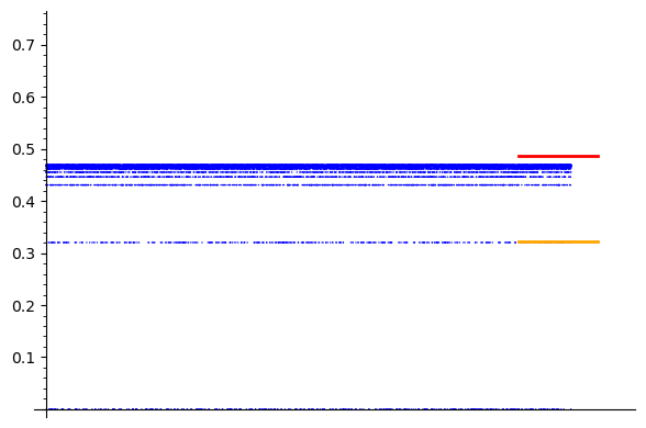

Prime orders. In Figure 8.2, the quantities corresponding to prime values of are marked in dark blue, and they seem to have a regular behavior for the two considered features. Indeed, both the ratio of height values near and their mean appear to follow hyperbola-like patterns, at least for large enough. Moreover, these patterns seem to bound, respectively from above and from below, the corresponding quantity for a general . It would be interesting to explain these behaviors.
In fact, when is prime, even the single height values corresponding to -torsion points seem to be simpler and tamer than those for composite , as can be seen in Figure 8.3 for .
This figure and similar ones suggest that for every prime all the height values corresponding to nontrivial -torsion points lie below , and that when they are nonzero, they are at least as large as . In precise terms:
Question 8.4.
Let be a prime and with . Does it hold that
PART II
In this part we present an interpretation of Theorem 6.1 from the viewpoint of Arakelov geometry, that allows to recover it in a more intrinsic way using the interplay between arithmetic and convex objects from the Arakelov geometry of toric varieties.
The first main result here is Theorem 10.4, linking the limit height in Theorem 6.1 with the Arakelov height of the subscheme of defined by the linear polynomial with respect to suitable metrized line bundles. The second main result is Corollary 13.3, showing that this height agrees with the average of a piecewise linear function over the Archimedean amoeba of this subscheme, that can in turn be computed as a rational multiple of a quotient of special values of the Riemann zeta function.
The treatment of this second part of the article is less elementary and certainly not self-contained, building on the theory developed by Gillet and Soulé [GS90] and its refinement by Maillot [Mai00], and on its study in the toric situation by Burgos Gil, Philippon and the second named author [BPS14] and by the first named author [Gua18b]. We will recall the main objects and results that we will use, assuming that the reader has some working knowledge of these subjects, including the basics of complex analytic geometry and of integral models of schemes.
9. Semipositive metrics in complex geometry
Let be a projective complex manifold with sheaf of holomorphic functions . Let be a holomorphic line bundle on , that is, a locally free sheaf of -modules of rank . A (continuous) metric on is a rule that to every open subset of and every section of on assigns a continuous function
| (9.1) |
that is compatible with restrictions to smaller open sets, and verifies that
- (1)
for every we have that if and only if ,
- (2)
for every and we have that .
The pair is called a metrized line bundle on .
Remark 9.1.
To define a metric on , it is enough to give a compatible choice of functions as those in (9.1) for a family of nonvanishing sections of on open subsets that cover the whole of .
To a metrized line bundle on one can associate its first Chern current , which is the current of bidegree defined on any open subset of as
for any nonvanishing section on , where for a real-valued function we denote by the associated distribution, and the operators and are taken in the sense of currents. This current does not depend on the choice of the section because of the Lelong–Poincaré formula.
A metrized line bundle is semipositive (respectively smooth) if for every nonvanishing local section the function is plurisubharmonic (respectively smooth).
Example 9.2.
The trivial line bundle admits a trivial metric , which is that defined by setting, for each holomorphic function on an open subset of ,
The corresponding metrized line bundle is denoted by . Computing its first Chern current using the holomorphic function we verify that , and so this metrized line bundle is semipositive.
Example 9.3.
Let be the hyperplane line bundle of the complex projective space . There is a one-to-one correspondence between its global sections and the linear polynomials in the homogeneous coordinates of . For each global section we denote by the corresponding linear polynomial and then set
Since is generated by its global sections, this assignment determines through Remark 9.1 a metric on this line bundle, which is called the canonical metric of . The corresponding metrized line bundle is denoted by . It is semipositive [BPS14, Example 1.4.4] but not smooth.
Example 9.4.
Consider the function defined as
where denotes the compact torus of and its probability Haar measure. Its value at a given point is the Mahler measure of an affine polynomial, and so it is a well-defined real number.
The function is continuous and positive homogeneous of degree . Similarly as for the canonical metric in the preceding example, the Ronkin metric of is obtained by setting, for each global section ,
The corresponding metrized line bundle is denoted by .
Remark 9.5.
Ronkin metrics on line bundles on toric varieties were introduced in [Gua18b], and they can be defined from any choice of nonzero Laurent polynomial compatible with the fan of the toric variety. The metric in Example 9.4 agrees with that from Definition 5.5 of loc. cit. for the Laurent polynomial . As explained therein, it is semipositive.
Given a pure -dimensional analytic cycle of , we denote by its associated integration current and by its support. Let also be a family of semipositive metrized line bundles on . Then, Bedford–Taylor’s theory allows to construct a measure on , denoted by
and called the complex Monge–Ampère measure of and , see [Dem12, Sections III.3 and III.4] for its definition and basic properties. This measure is supported on , and has finite integral against functions with at most logarithmic singularities along analytic subsets of of lower dimension. In particular, it gives zero mass to those analytic subsets. Finally, this measure is positive whenever is effective.
The next proposition is a particular case of well-known results in analytic geometry, see for instance [BE21, Lemma 8.17(ii)]. It is also a direct consequence of the commutativity of the -product from Arakelov geometry shown in [GS90, Corollary 2.2.9] and extended in [Mai00, Proposition 5.3.6] to metrized line bundles that are not necessarily smooth. We include its proof for convenience and greater clarity.
Proposition 9.6 (metric Weil reciprocity law).
Let be a smooth projective complex curve. For , let also be a semipositive metrized line bundle on , and a nonzero rational section of . Suppose that the -cycles
have disjoint supports. Then
| (9.2) |
Proof.
Both sides of the formula in (9.2) are linear in the choice of the metrized line bundles and rational sections. Hence we can assume that and are ample. When this is the case, their metrics can be uniformly approached by smooth semipositive metrics on the same line bundles. Since both sides of this formula are continuous with respect to the uniform convergence of metrics, we can then reduce to the case in which both and are smooth. We suppose this for the rest of the proof.
For each choose a closed neighborhood with smooth boundary. Assume that all of these neighborhoods are disjoint and consider the open subset with smooth boundary
Set for each . Since the rational section is regular and nonvanishing on and the metric is smooth, the restriction to of the complex Monge–Ampère measure is given by the -form . By [Dem12, Chapter III, Formula 3.1],
| (9.3) |
Note that the integral in the left-hand side of (9.3) approaches the same integral over the whole of when all the considered neighborhoods get arbitrarily small.
By spelling out the different connected components of we obtain that
| (9.4) |
The first sum in the right-hand side of (9.4) tends to when these neighborhoods get small, as is a smooth -form on for every and has a logarithmic singularity at every such point.
Now let . Choosing the neighborhood appropriately, we can suppose that there is a closed disc centered at the origin together with a biholomorphic map such that . Then for and a nonvanishing smooth function . Hence
| (9.5) |
Since is a smooth -form on , the second summand in the right-hand side of (9.5) tends to when shrinks to the point . For the first summand, recall that with and the Dolbeault operators. Hence
and noting that the function is real-valued we deduce that
| (9.6) |
Since contains no point of , the function is smooth on . Then Cauchy’s formula [Dem12, Chapter I, Formula 3.2] gives
| (9.7) |
where denotes the Lebesgue measure of . As shrinks to , the integral in the right-hand side of (9.7) converges to because the function is integrable on , and so the integral in the left-hand side tends to . From (9.5) and (9.6) we deduce that converges to .
Remark 9.7.
The classical Weil reciprocity law is the equality
| (9.8) |
for any pair of nonzero rational functions and of a smooth projective curve whose associated -cycles have disjoint support [Sil09, Exercise 2.11].
Proposition 9.6 can be seen as a metric version of this reciprocity law, that essentially contains it. Indeed choosing both and as the trivial metrized line bundle of from Example 9.2, this proposition yields the equality between the absolute values of the right-hand and left-hand sides of (9.8).
10. The limit height of the intersection as an Arakelov height
In this section we link Theorem 6.1 to the theory of heights from Arakelov geometry. To this end, we first recall the basic elements of this theory for arithmetic varieties equipped with semipositive metrized line bundles that are not necessarily smooth.
Let be an arithmetic variety, that is a regular integral projective flat scheme over , with sheaf of regular functions . By the regularity assumption, its set of complex points is a projective complex manifold. Given a line bundle on , its analytification is a holomorphic line bundle on .
A semipositive metrized line bundle on is a pair
where is a line bundle on and a semipositive metric on that is invariant under the involution on induced by the complex conjugation. We denote by the associated semipositive metrized line bundle on .
For a pure -dimensional cycle of and a family of semipositive metrized line bundles for , on , we define its (Arakelov) height
by means of the following recursion on the dimension:
- (1)
when , if is a prime cycle then it is an integral closed point of and its function field is finite. In this case its height is defined as
In the general case, the height of is defined by linearity.
- (2)
when , pick a rational section of that is regular and nonvanishing on a dense open subset of the support of and set
where denotes the intersection product of the Cartier divisor and the cycle , and stands for considered as a meromorphic section of .
The height is a real number that does not depend on the choice of the rational section in (2) nor on the order in which the metrized line bundles are chosen.
Remark 10.1.
Example 10.2.
Let be the projective space over . The pair
where denotes the hyperplane line bundle of and the canonical metric of the holomorphic line bundle from Example 9.3 is a semipositive metrized line bundle on this arithmetic variety, called the canonical metrized line bundle of .
Let be the projective space introduced in Section 1. A point with rational homogeneous coordinates can be identified with a -point of or equivalently with a scheme-theoretic point in its generic fiber. Denote by its closure in , which is an integral subscheme of dimension . Then
| (10.1) |
the quantity on the right-hand side being the height of in the sense of (1.6). Proving this equality is a nice exercise that can be solved by unwrapping the corresponding definitions and by using Remark 1.1.
Remark 10.3.
More generally, the Arakelov height can be defined for cycles of , the base change of with respect to the integral closure of the ring of integers. In this setting, a point can be identified with a -point of or equivalently with a scheme-theoretic point in the generic fiber of . The equality in (10.1) extends then to and its closure in .
Now consider the semipositive metrized line bundles on
| (10.2) |
obtained by equipping the holomorphic line bundle on with the canonical and the Ronkin metrics from Examples 9.3 and 9.4, respectively. Consider also the subscheme of defined by the homogeneous linear polynomial . The line studied through Part I coincides with the set of -points of .
The following is our main result in this section.
Theorem 10.4.
Let be a strict sequence in of nontrivial torsion points. Then
Its proof relies on the next complex analytic equality. As in Section 4 we denote by the compact torus of and by its probability Haar measure.
Lemma 10.5.
Let be the global section of corresponding to the homogeneous coordinate of . Then
Proof.
Set for short . By construction, it is a measure on supported on the line . For each we consider the integral
| (10.3) |
which is finite because the restriction of the integrand to this line is a function which is continuous at all but two points, where it has at most logarithmic singularities.
We will find a simpler expression for this integral as an application of the metric Weil reciprocity law. To this end, consider the inclusion and the semipositive metrized line bundles on given by the inverse image with respect to this map of the trivial and the canonical metrized line bundles on , that is
On the one hand, the rational function of restricts to a nonzero rational function of , which gives a nonzero rational section of . On the other hand, given complex numbers and not both equal to , the linear polynomial corresponds to a global section of , which restricts to the nonzero global section of . The -cycles of respectively defined by these pulled-back rational sections are
| (10.4) |
For an appropriate choice of and , the supports of these -cycles are disjoint.
The restriction of the measure to the line coincides with , by the functoriality of the Monge–Ampère operator. Moreover , as shown in Example 9.2. Hence Proposition 9.6 together with (10.3) and (10.4) implies that
| (10.5) |
We have that
Hence (10.5) simplifies to
| (10.6) |
in accordance with the notation in (4.1).
We now consider the functions defined as
whenever , and as and arbitrary constant otherwise. The subset has zero mass with respect to the product measure , and so the integrals of these functions on do not depend on the choice of this constant.
The function is constant with respect to the first variable, whereas, as a function of the second one, its restriction to the line only has a logarithmic singularity at a point, making it integrable with respect to . Moreover is nonnegative, and from (10.3) and (10.6) we deduce that the iterated integral
is finite. Tonelli’s theorem then implies that the function , and a fortiori , is integrable with respect to the product measure , and that
| (10.7) |
Proof of Theorem 10.4.
By Corollary 3.6 and Proposition 4.1,
On the other hand, the recursive definition of the Arakelov height shows that
The divisor coincides with the -dimensional irreducible subscheme of arising as the Zariski closure of the point in the generic fiber of this scheme corresponding to the point . So (10.1) gives
The statement then follows from Lemma 10.5. ∎
11. A toric perspective
The rest of the article is concerned with expressing and computing the Arakelov height in Theorem 10.4 in terms of convex geometry through the theory of heights of toric varieties and of their hypersurfaces, respectively studied in [BPS14] and in [Gua18b]. Since the only toric variety that we need to consider here is the projective space, we restrict our presentation to this specific case. In spite of that, this is sufficient to give a taste of the general theory.
Let be a convex subset and a concave function on it, that is a function satisfying
Its stability set is the subset of defined as
where denotes the usual scalar product. Then the Legendre–Fenchel dual of is the function defined as
It is concave and upper semicontinuous. If is upper semicontinuous, then .
Example 11.1.
Let be the standard simplex of , that is the -dimensional simplex whose vertices are the origin and the vectors in the standard basis of this vector space. Its support function is the function defined as
It is piecewise linear and concave, its stability set coincides with , and its Legendre–Fenchel dual is , the zero function on this simplex.
Example 11.2.
Let be the compact torus of and its probability Haar measure. The Ronkin function is the function defined as
It is linked to the function in Example 9.4 by the relation
| (11.1) |
The function is concave and its difference with the support function is uniformly bounded [Gua18b, Proposition 2.10]. This implies that its stability set is the standard simplex and that its Legendre–Fenchel dual is a continuous concave function on it.
Remark 11.3.
Ronkin functions can be associated to any Laurent polynomial, or more generally to any holomorphic function on an open and -invariant subset of . As such, they were introduced by Ronkin in [Ron01] and further investigated by Passare and Rullgård in [PR04].
Up to its sign, the function in Example 11.2 is the special case corresponding to the Laurent polynomial . For , Cassaigne and Maillot have found an explicit expression for it in terms of the Bloch–Wigner dilogarithm [Mai00, Proposition 7.3.1]. In spite of being our case of interest, we do not need such a description in this article.
The importance of concave functions in our context stems from their interplay with semipositive toric metrics on the hyperplane line bundle of the complex projective space. A metric on is toric if
| (11.2) |
where denotes the translation of by as in (1.3) and the global section of corresponding to the homogeneous coordinate of .
To a toric metric on one can associate its metric function, which is the function defined as
A toric metric on is semipositive if and only if its metric function is concave [BPS14, Theorem 4.8.1(1)]. When this is the case, the stability set of this concave function is the standard simplex , and one also associates to the toric metric its roof function, which is the continuous concave function
defined as the Legendre–Fenchel dual of .
Example 11.4.
The canonical metric of from Example 9.3 is toric, as it can be readily checked from the condition in (11.2), and its metric function coincides with the support function from Example 11.1. This recovers the semipositivity of and implies that its roof function is the zero function .
Example 11.5.
The Ronkin metric of from Example 9.4 is also toric by definition, and the associated metric function agrees with the Ronkin function from Example 11.2, by means of the relation (11.1). In particular, it is a semipositive metric on having as roof function its Legendre–Fenchel dual .
The main results of [BPS14] and [Gua18b] allow to express the height of and of its hypersurfaces with respect to a family of semipositive toric metrics on in terms of its associated family of roof functions. This is achieved through the mixed integral , which is an operator on families of -many continuous concave functions on compact convex subsets of that is obtained by polarizing the usual integral operator [BPS14, Definition 2.7.16].
Since our case of interest is , we adapt the statements from the adelic setting of the loc. cit. to the schematic point of view of the present paper to obtain the following.
Proposition 11.6.
Let and be the canonical and Ronkin metrized line bundles of as in (10.2), and the subscheme defined by the linear polynomial . Then
Proof.
This proof assumes a working knowledge of the adelic approach to the theory of Arakelov heights as exposed in [BPS14, Chapter 1].
Let be the projective plane over and the Cartier divisor of the line at infinity. The pair is an integral model of , and so the canonical and the Ronkin metrized line bundles on induce quasi-algebraic semipositive adelic metrized divisors
on in the sense of [BPS14, Section 1.5]. Namely, their Archimedean metrics coincide respectively with those of and , and so do their Archimedean roof functions. Instead, their non-Archimedean metrics are those induced by the integral model as in [BPS14, Example 1.3.11], and then their roof functions agree with the zero function on .
This correspondence is compatible with the associated heights, and thus [BPS14, Theorem 5.2.5] together with Examples 11.4 and 11.5 specializes to
which gives the second equality in the statement. We also have that
because contains no vertical component, and [Gua18b, Theorem 5.12] gives
as coincides with the Ronkin metrized divisor of the Laurent polynomial in the sense of [Gua18b]. This gives the first equality and completes the proof. ∎
Combining this result with Theorem 10.4 and the equality in (10.1) yields the following statement.
Corollary 11.7.
Let be a strict sequence in of nontrivial torsion points. Then
where denotes the -dimensional subscheme of defined by these linear forms.
This limit formula is a particular case of a conjectural arithmetic analogue of the geometric fact that for a family of -many line bundles on an -dimensional algebraic variety, the cardinality of the zero set of a generic -tuple of their global sections coincides with the degree of the variety with respect to these line bundles. Formulating this conjecture requires the language of adelic metrized line bundles on varieties over global fields, which would take us too far away from our setting. Instead, we content ourselves by explaining a particular case that can be expressed with the objects at hand and still gives a hint of the general case.
For , consider the -tensor power line bundle on . Its global sections are in one-to-one correspondence with the homogeneous polynomials of degree in the homogeneous coordinates of this projective space. Extending Example 9.4, we define the Ronkin metric of setting, for each global section ,
where is the homogeneous polynomial of degree corresponding to , and is the same function as that of the referred example. This metric is toric and semipositive, and the corresponding metrized line bundle on is denoted by .
Conjecture 11.8.
Let be a strict sequence in of nontrivial torsion points. Then for we have that
In contrast with Corollary 11.7, this statement would allow to predict this kind of limit heights in situations where the considered systems of equations cannot be explicitly solved.
12. Integrals over an amoeba
In Section 4 we considered the co-tropicalization map on that sends each point to the arguments of its coordinates. Looking instead at their absolute values gives the more classical tropicalization map:
The image of a curve of under this map is called its amoeba. The term was coined in [GKZ08, Section 6.1], where these tentacle-shaped subsets were introduced.
Here we will be concerned with the amoeba of the curve of defined by the Laurent polynomial , that is
| (12.1) |
We will refer to this subset of as the Archimedean amoeba of , the line of studied throughout Part I. It is depicted in Figure 12.1, and its computation is explained in [Gua20].
Remark 12.1.
This terminology can be justified as follows. The line is defined over the rationals, and so it can be identified with an integral subscheme of whose Archimedean analytification is the complex line . Then the subset coincides with the amoeba of the restriction of this complex line to the dense open subset .
For the sequel, consider the subset of this Archimedean amoeba given as
which is the region colored in dark blue in Figure 12.1. The next result shows that the integrals on this region of the powers of a coordinate function are given by special values of the Riemann zeta function.
Proposition 12.2.
For all we have that
Proof.
The nontrivial boundary of the region is given by , as indicated in Figure 12.1. Then Tonelli’s theorem and a direct computation yield
| (12.2) |
The absolute convergence of the series for the logarithm on the open unit disk and the obvious statement for imply the pointwise convergence
as functions with values in . Since every summand of the series has the same sign, Levi’s monotone convergence theorem implies that
| (12.3) |
This result can be employed to recover the computation of the area of by Passare and Rullgård in [PR04, page 502]. A similar computation appears in [KP16, page 919].
Example 12.3.
For , Proposition 12.2 gives that . Note that is disjointly covered, up to subsets of measure zero, by the images of the south region under the map and under the symmetry along the diagonal. Since these maps preserve the Lebesgue measure, we deduce that
The previous proposition also allows to compute the integral on the Archimedean amoeba of of the support function of the -dimensional standard simplex.
Example 12.4.
For , Proposition 12.2 gives that . Consider the subsets of defined as
Then
where the second equality follows from the symmetries of this integral.
Remark 12.5.
It would be interesting to explore if there are other integrals of piecewise polynomial functions on amoebas of curves that can be expressed in terms of special values of -functions.
13. Computing a mixed integral
Finally, we show how the mixed integral in Proposition 11.6 relates to the integral of a piecewise linear function on the amoeba treated in Section 12. The obtained equality offers a further expression for the limit height under study, and it can be used to recover our main result.
Set for the standard simplex of and denote by the zero function on it. Set also for the support function of this simplex as in Example 11.1, and for the Ronkin function of according to Example 11.2. Recall that denotes the Archimedean amoeba of the line as in (12.1).
Theorem 13.1.
With notation as above, we have that
where denotes the Lebesgue measure of .
To prove this result, we first need to understand the behavior of the Legendre–Fenchel dual of this Ronkin function on the boundary of its domain.
Lemma 13.2.
The function vanishes on the boundary of .
Proof.
It is a consequence of Jensen’s formula that
| (13.1) |
see for instance [Mai00, Proposition 7.3.1(2)]. Since is concave, this implies that the inequality holds on the entire real plane. Taking Legendre–Fenchel duals we obtain that for all .
Hence, to complete the proof it is enough to show that is nonpositive on the boundary of . To this aim, first consider a point with . For the point belongs to the east border of , as shown in Figure 12.1. By (13.1) and the continuity of the Ronkin function we necessarily have that . Hence
which implies that . The fact that this also holds when with can be proven similarly.
To conclude, let with . For consider the point , which lies in the southern border of . Again by (13.1) and the continuity of the Ronkin function we have that . Hence
which implies that also holds in this case, as stated. ∎
We can now move to the proof of Theorem 13.1, which relies on a relation between the mixed integral and an integral on the dual space with respect to the real Monge–Ampère measure of a concave function. The latter is a positive measure having higher density where the function is more concave [BPS14, Definition 2.7.1].
Proof of Theorem 13.1.
Since both and are continuous concave functions on the simplex of , it is a consequence of [Gua18b, Theorem 1.6] together with the vanishing of on the boundary of shown in Lemma 13.2 that
| (13.2) |
where stands for the real Monge–Ampère measure of the Ronkin function.
By [PR04, Theorem 7 and Example on page 502] the real Monge–Ampère measure of agrees with the Lebesgue measure of restricted to the amoeba , and scaled by the constant , and so
| (13.3) |
The statement follows from (13.2) and (13.3) together with Example 12.3. ∎
The following corollary is an immediate consequence of the chain of equalities given by Theorem 10.4, Proposition 11.6 and Theorem 13.1.
Corollary 13.3.
Let be a strict sequence in of nontrivial torsion points. Then
where is the subscheme of defined by , whereas and are the canonical and Ronkin semipositive metrized line bundles on .
This result highlights the role played by our particular choice of both height function and curve. Indeed, the considered limit height turns out to be computed by the average of , which is metric function associated to the canonical height in the toric correspondence from [BPS14], on the Archimedean amoeba of the line .
Finally, the right-hand side in the equalities in Corollary 13.3 can be directly computed using Examples 12.3 and 12.4, namely
thus recovering Theorem 6.1 through this more conceptual point of view.
References
- [BE21] S. Boucksom and D. Eriksson, Spaces of norms, determinant of cohomology and Fekete points in non-Archimedean geometry, Adv. Math. 378 (2021), Paper No. 107501, 124 pp.
- [BG06] E. Bombieri and W. Gubler, Heights in Diophantine geometry, New Math. Monogr., vol. 4, Cambridge Univ. Press, 2006.
- [BGS94] J.-B. Bost, H. Gillet, and C. Soulé, Heights of projective varieties and positive Green forms, J. Amer. Math. Soc. 7 (1994), 903–1027.
- [Bil97] Y. Bilu, Limit distribution of small points on algebraic tori, Duke Math. J. 89 (1997), 465–476.
- [BPRS19] J. I. Burgos Gil, P. Philippon, J. Rivera-Letelier, and M. Sombra, The distribution of Galois orbits of points of small height in toric varieties, Amer. J. Math. 141 (2019), 309–381.
- [BPS14] J. I. Burgos Gil, P. Philippon, and M. Sombra, Arithmetic geometry of toric varieties. Metrics, measures and heights, Astérisque, vol. 360, Soc. Math. France, 2014.
- [BZ20] F. Brunault and W. Zudilin, Many variations of Mahler measures — a lasting symphony, Austral. Math. Soc. Lect. Ser., vol. 28, Cambridge Univ. Press, 2020.
- [Col93] P. Colmez, Périodes des variétés abéliennes à multiplication complexe, Ann. of Math. (2) 138 (1993), 625–683.
- [CT09] A. Chambert-Loir and A. Thuillier, Mesures de Mahler et équidistribution logarithmique, Ann. Inst. Fourier (Grenoble) 59 (2009), 977–1014.
- [Dem12] J.-P. Demailly, Complex analytic and differential geometry, book available at https://www-fourier.ujf-grenoble.fr/~demailly/manuscripts/agbook.pdf, 2012.
- [DH19] V. Dimitrov and P. Habegger, Galois orbits of torsion points near atoral sets, e-print arXiv:1909.06051, 2019.
- [DP99] S. David and P. Philippon, Minorations des hauteurs normalisées des sous-variétés des tores, Ann. Scuola Norm. Sup. Pisa Cl. Sci. (4) 28 (1999), 489–543.
- [GKZ08] I. M. Gelfand, M. M. Kapranov, and A. V. Zelevinsky, Discriminants, resultants and multidimensional determinants, Math. Theory Appl., Birkhäuser, 2008.
- [GS90] H. Gillet and C. Soulé, Arithmetic intersection theory, Inst. Hautes Études Sci. Publ. Math. 72 (1990), 93–174.
- [GS22] R. Gualdi and M. Sombra, Computing the height of the intersection of the line and its translate by a torsion point, SageMath notebook available at https://bit.ly/3GFNAcB, 2022.
- [Gua18a] R. Gualdi, Height of cycles in toric varieties, Ph.D. thesis, U. Bordeaux and U. Barcelona, 2018.
- [Gua18b] by same author, Heights of hypersurfaces in toric varieties, Algebra Number Theory 12 (2018), 2403–2443.
- [Gua20] by same author, The amoeba of a planar line, note available at https://homepages.uni-regensburg.de/~gur23971/documents/Amoeba_of_hyperplane.pdf, 2020.
- [GZ86] B. H. Gross and D. Zagier, Heegner points and derivatives of -series, Invent. Math. 84 (1986), 225–320.
- [Har98] G. Harman, Metric number theory, London Math. Soc. Monogr. (N.S.), vol. 18, Oxford Univ. Press, 1998.
- [JJ56] H. Jeffreys and B. S. Jeffreys, Methods of mathematical physics, third ed., Cambridge Univ. Press, 1956.
- [KP16] J. Kramer and A.-M. von Pippich, Snapshots of modern mathematics from Oberwolfach: special values of zeta functions and areas of triangles, Notices Amer. Math. Soc. 63 (2016), 917–922.
- [Lan94] S. Lang, Algebraic number theory, second ed., Grad. Texts Math., vol. 110, Springer-Verlag, 1994.
- [Mai00] V. Maillot, Géométrie d’Arakelov des variétés toriques et fibrés en droites intégrables, Mém. Soc. Math. Fr. (N.S.) 80 (2000), vi+129 pp.
- [MR02] V. Maillot and D. Roessler, Conjectures sur les dérivées logarithmiques des fonctions d’Artin aux entiers négatifs, Math. Res. Lett. 9 (2002), 715–724.
- [MS19] C. Martínez and M. Sombra, An arithmetic Bernštein-Kušnirenko inequality, Math. Z. 291 (2019), 1211–1244.
- [Neu99] J. Neukirch, Algebraic number theory, Grundlehren Math. Wiss., vol. 322, Springer-Verlag, 1999.
- [Nor50] D. G. Northcott, Periodic points on an algebraic variety, Ann. of Math. (2) 51 (1950), 167–177.
- [PP20] F. Pazuki and R. Pengo, On the Northcott property for special values of L-functions, e-print arXiv:2012.00542, 2020.
- [PR04] M. Passare and H. Rullgård, Amoebas, Monge-Ampère measures, and triangulations of the Newton polytope, Duke Math. J. 121 (2004), 481–507.
- [Ron01] L. I. Ronkin, On zeros of almost periodic functions generated by functions holomorphic in a multicircular domain (Russian), Complex analysis in modern mathematics, FAZIS, 2001, pp. 239–251.
- [Sag22] Sage Developers, Sagemath, the Sage mathematics software system (version 9.7), https://www.sagemath.org, 2022.
- [Sil09] J. H. Silverman, The arithmetic of elliptic curves, second ed., Grad. Texts Math., vol. 106, Springer, 2009.
- [Smy81] C. Smyth, On measures of polynomials in several variables, Bull. Austral. Math. Soc. 23 (1981), 49–63.
- [Wei51] A. Weil, Arithmetic on algebraic varieties, Ann. of Math. (2) 53 (1951), 412–444.
- [Zag93] D. Zagier, Algebraic numbers close to both and , Math. Comp. 61 (1993), 485–491.