Consolidated Control Barrier Functions: Synthesis and Online Verification via Adaptation under Input Constraints

• •

  We formalize the notion of a consolidated CBF (C-CBF) by proposing a generic class of candidate functions that smoothly synthesizes any arbitrary number of time-varying constraint functions into one.

• •

  We utilize a predictor-corrector interior point method to propose an optimization-based adaptation law for the weights of the C-CBF candidate’s constituent functions. We show that the resulting weights render the C-CBF forward invariance condition viable at all times despite limited control authority, which serves to certify the C-CBF candidate as valid and permits the use of existing approaches to CBF-based control design for a class of nonlinear, control-affine systems.

• •

  We illustrate the performance of our approach on a one-dimensional, academic example which requires the controller to recognize and avoid regions of the state space in which the specified constraints are satisfied, but where no control input is able to prevent the constraints from being violated in the future.

• •

  Finally, we provide a comparative example utilizing a (car-like) robot with bicycle dynamics to highlight how our proposed controller solves a reach-avoid problem in which two baseline controllers fail, and highlight how the weight adaptation ensures that constraints are satisfied independent of their relative-degree.

In our prior work [35], we introduced an adaptation law for rendering a similar form of consolidated CBF viable with respect to time-invariant constraint functions under unbounded control authority. Previously, the parameter adaptation law was taken to be the solution to a QP, as opposed to the predictor-corrector interior point method introduced in this paper. In addition, we extend our previous framework to handle spatiotemporal constraints (i.e., time-varying) and a class of input constraints. In this sense, the work herein has not been proposed to any other venue.

The paper is organized as follows. Section II introduces some preliminaries, including time-varying convex optimization and constrained control design with CBFs. In Section III, we introduce the form of our C-CBF and propose a parameter adaptation law for rendering it valid. Section IV introduces our proposed QP-based control law, the performance of which we demonstrate with two simulation examples in Section V. In Section VI we conclude with final remarks and directions for future work.

Consider a time-varying, possibly non-convex optimization problem, a local solution trajectory to which takes the form

where $J:\R\times\R^{p}\rightarrow\R$ is a (uniformly strongly convex) objective function, the collection of $q\geq 0$ (not necessarily convex) inequality constraints is $c_{i}:\R\times\R^{p}\rightarrow\R$ for $i\in[q]$, and where all of $J$ and $c_{i}$ are twice continuously differentiable in $\boldsymbol{y}$ and piecewise continuously differentiable in $t$. Denote the feasible region of (1) as $\mathcal{Y}(t)=\{\boldsymbol{y}\in\R^{p}:c_{i}(t,\boldsymbol{y})\leq 0,\forall i\in[q]\}$, and further assume that the feasible region has an interior point at all times, i.e., that $\mathrm{Int}(\mathcal{Y}(t))\neq\emptyset$, $\forall t\geq 0$. Though $J$ is assumed to be uniformly strongly convex, without convexity of the inequality constraints it is not guaranteed that (1) is the global solution trajectory; nevertheless, barrier function methods may be employed to approximate a local solution (1) (see e.g., [36, Sec. 9.4]). Consider such an approximate solution $\hat{\boldsymbol{y}}^{*}(t)$, constructed using Frisch’s logarithmic barrier functions:

where $s>0$ is a barrier design parameter. In the limit, as $s\rightarrow\infty$, the function $-\frac{1}{s}\log(-c_{i}(t,\boldsymbol{y}))\rightarrow\mathbb{I}_{-}(c_{i}(t,\boldsymbol{y}))$, where $\mathbb{I}_{-}:\R\rightarrow\{0,\infty\}$ is defined such that $\mathbb{I}_{-}(u)=0$ for $u\leq 0$ and $\mathbb{I}_{-}(u)=\infty$ for $u>0$. In addition to facilitating this non-smooth function approximation, the barrier parameter may also convexify the augmented objective function $\Psi$. Though $\log(-c_{i})$ may be non-convex, we assume (similar to e.g., [37]) that for sufficiently large $s$ the function $\Psi$ is strongly, uniformly convex, stated formally as follows.

In practice, for strongly uniformly convex $J$ the above may be satisfied by using sufficiently large $s$, which may be determined either online or iteratively offline. It follows then that $\nabla_{\boldsymbol{yy}}\Psi$ exists and is bounded, which allows us to review a version of [38, Lemma 2] relating the approximate (locally) optimal trajectory $\hat{\boldsymbol{y}}^{*}(t)$ given by (2) to the solution of a continuous-time dynamical system.

The above result implies that the solution $\boldsymbol{z}(t)$ to (3) approaches the approximate optimal trajectory $\hat{\boldsymbol{y}}^{*}(t)$ asymptotically while remaining in the feasible region $\mathcal{Y}(t)$ at all times. Intuitively, the dynamics of (3) consist of a prediction term

and a Newton-like correction term

which together ensure that $\boldsymbol{z}(t)\in\mathrm{Int}(\mathcal{Y}(t))$ at all times (hence predictor-corrector interior point method). We require the findings from Lemma 1 in the proof of one of our main results on parameter adaptation for constrained control design, the premises of which we will now review.

In the remainder of this paper we consider a class of nonlinear, control-affine dynamical systems of the form

where $t\in\mathcal{T}=[t_{0},\infty)$ represents time, $\boldsymbol{x}\in\R^{n}$ and $\boldsymbol{u}\in\mathcal{U}\subset\R^{m}$ are the state and control input vectors, with $\mathcal{U}$ the input constraint set, and where $f:\R^{n}\rightarrow\R^{n}$ and $g:\R^{n}\rightarrow\R^{n\times m}$ are known and locally Lipschitz. The input constraint set is

where the inequalities are interpreted element-wise and $\boldsymbol{u}_{max}=(\bar{u}_{1},\cdots,\bar{u}_{m})$ with $0<\bar{u}_{j}<\infty$ for $j\in[m]$. We assume the availability of a control input $\boldsymbol{u}:\mathcal{T}\rightarrow\mathcal{U}$ that yields a unique solution to (4) for all $t\in\mathcal{T}$.

Consider one of $c\geq 1$ (possibly time-varying) twice continuously differentiable constraint functions $h_{i}:\mathcal{T}\times\R^{n}\rightarrow\R$, which may encode a safety, performance, and/or specification based constraint, and let the set of states over which this particular constraint is satisfied at a given time $t$ be

We denote the set of all constraint functions as

and in this paper focus on confining the state to the intersection of all individual constraint sets, hereafter referred to as the complete constraint set:

We assume that the complete constraint set possesses an interior point, i.e $\mathrm{Int}(\mathcal{S}(t))\neq\emptyset$, $\forall t\in\mathcal{T}$, and thus seek to design a controller that renders a subset $\mathcal{D}(t)\subseteq\mathcal{S}(t)$ forward-invariant with respect to the system (4), i.e., to ensure that $\boldsymbol{x}(0)\in\mathcal{D}(0)\subseteq\mathcal{S}(0)\implies\boldsymbol{x}(t)\in\mathcal{D}(t)\subseteq\mathcal{S}(t)$, $\forall t\in\mathcal{T}$. Of note is that we require that the functions $h_{i}$ be twice continuously differentiable, a stricter (though often reasonable) condition than the more typical continuous differentiability requirement, for reasons pertaining to our parameter adaptation law in Section III.

For the remainder of this section we will introduce preliminaries specific to the case of one constraint function ($c=1$). Under such circumstances, one approach to controlled set invariance is to use CBFs in the control design. We now review the notion of a time-varying CBF inspired by [39, 22], and highlight how it is used to enforce forward-invariance.

We refer to (9) as the CBF condition, and note that if the function $h_{i}$ has relative-degree¹¹ 1 A function $p:\R_{+}\times\R^{n}\rightarrow\R$ is said to be of relative-degree $r$ with respect to the dynamics (4) if $r$ is the number of times $p$ must be differentiated before one of the control inputs $u$ appear explicitly. $r>1$ with respect to the system (4) then the control input $\boldsymbol{u}$ has no effect on (9). In many cases this deficiency can be resolved by deriving high-order CBFs (see e.g., [16, 3] for details), though this may require careful parameter design [40]. The method we propose in Section III, however, requires no assumptions about the relative-degree of the constraint functions under consideration, a fact that we highlight in our second numerical case study in Section V. For a particular constraint function $h_{i}$, we refer to the set of control actions satisfying its CBF condition (9) as its CBF control set and denote it by

noting that $\mathcal{U}_{h_{i}}$ is parameterized by the set function $\alpha\in\mathcal{K}_{\infty}$. In the following result inspired by [22], it is shown that controls belonging to the CBF control set $\mathcal{U}_{h_{i}}$ render the constraint set $\mathcal{S}_{i}(t)$ forward-invariant.

The main open problem in constrained control design under multiple state and input constraints is in certifying that all constraints will satisfied jointly in perpetuity. We bridge this gap by 1) synthesizing one consolidated CBF (C-CBF) candidate from the collection of constraints and then 2) certifying the C-CBF candidate as valid via online parameter adaptation.

We refer to the new constraint function $H$ as a C-CBF candidate, and seek to guarantee that we can render its zero super-level set $\mathcal{D}(t,\boldsymbol{w})$ forward-invariant in the presence of input constraints of the form (5). Consolidating many separate constraint functions $h_{i}$ into one function $H$ means that each weight $w_{i}$ affects the relative importance of $h_{i}$ in $H$ (and by extension on the set $\mathcal{D}$). It also allows us, however, to leverage existing CBF results for certifiable constrained control design. Notably, we may then use the class of QP based controllers (11) with the new function $H$ to render $\mathcal{D}$ forward-invariant and thus to ensure that the state remains within the complete constraint set $\mathcal{S}$. Proving that $H$ is a valid C-CBF, however, may be difficult when using static constituent function weights $\boldsymbol{w}$, i.e., weights chosen a priori with $\dot{\boldsymbol{w}}\equiv\mathbf{0}_{c\times 1}$. We therefore seek to design a weight adaptation law $\dot{\boldsymbol{w}}=\omega(t,\boldsymbol{w},\boldsymbol{x},\boldsymbol{u})$, $\omega:\mathcal{T}\times\R_{+}^{c}\times\R^{n}\times\mathcal{U}\rightarrow\R^{c}$, that varies the weights $\boldsymbol{w}$ online and, in doing so, renders the C-CBF candidate $H$ valid. With $\boldsymbol{w}$ then dependent on time $t$, in the remainder we omit the dependence of $\mathcal{D}$ on the weights $\boldsymbol{w}$ for conciseness. To render the C-CBF candidate $H$ valid is to ensure that

holds for all $\boldsymbol{x}(t)\in\mathcal{D}(t)$, $\forall t\in\mathcal{T}$. Notice that the above is to the C-CBF candidate $H$ as (9) is to a CBF candidate $h_{i}$. Thus, we refer to (15) as the C-CBF condition. While we have established that the CBF condition (9) is affine in the control input $\boldsymbol{u}$ for the class of systems described by (4), the C-CBF condition (15) is only affine in $\boldsymbol{u}$ if the adaptation law $\dot{\boldsymbol{w}}$ is affine in (or independent of) $\boldsymbol{u}$, i.e., if $\dot{\boldsymbol{w}}$ takes the form

for some functions $\mu:\mathcal{T}\times\R_{+}^{c}\times\R^{n}\rightarrow\R^{c}$ and $\nu:\mathcal{T}\times\R_{+}^{c}\times\R^{n}\rightarrow\R^{c\times m}$. With $\dot{\boldsymbol{w}}$ taking this form, we may directly include the C-CBF condition (15) as a linear constraint in a QP-based control law of the form (11). As such, we now formally introduce the second problem under consideration.

Notice that (18) constitutes a sufficient condition for the satisfaction of the C-CBF condition (15), and therefore ensures that the CBF control set $\mathcal{U}_{H}(t,\alpha)$ is never empty.

The form of our C-CBF candidate $H:\mathcal{T}\times\R^{c}_{+}\times\R^{n}\rightarrow\R$ is

where $\phi:\R_{+}\times\R_{+}\rightarrow\R_{+}$ belongs to class-$\mathcal{L}\mathcal{L}$, is twice continuously differentiable, and satisfies $\phi(r,0)=\phi(0,s)=\phi(0,0)=1$. Note that the specified domain considers only positive values for $w_{i}$ and $h_{i}$, a reasonable choice since $\boldsymbol{x}(t)\notin\mathcal{D}(t)$ if some $h_{i}(t,\boldsymbol{x}(t))\leq 0$ with $w_{i}\geq 0$ or if some $w_{i}\leq 0$ with $h_{i}(t,\boldsymbol{x}(t))\geq 0$. Both the decaying exponential function $\phi(r,s)=e^{-rs}$ and the class of reciprocal functions of the form $\phi(r,s)=v/(rs+v)$, $v>0$, for example, satisfy the above requirements over the admissible domain. The function $\phi$ thus encodes that the zero super-level set of $H$ is a subset of the complete constraint set $\mathcal{S}(t)$, i.e.,

provided that $\boldsymbol{w}\in\R^{c}_{+}$. Note that the weights behave as a shape parameter for the function $\phi$, and are neither used to construct a weighted average nor required to sum to any specific amount. Instead, observe that larger weights $\boldsymbol{w}$ allow $\mathcal{D}(t)$ to more closely approach $\mathcal{S}(t)$, as for a given state it follows that $\phi(h_{i}(t,\boldsymbol{x}),w_{i}^{l})<\phi(h_{i}(t,\boldsymbol{x}),w_{i}^{s})$ for $w_{i}^{l}>w_{i}^{s}>0$. This means that a higher weight $w_{i}$ confers smaller relative importance of its associated constraint function $h_{i}$ to the C-CBF candidate $H$. For example, in Figure 2 the effect of two different weights on the level sets of two obstacle avoidance constraint functions is depicted. In this case, obstacle two has smaller relative importance (i.e., $w_{2}>w_{1}$) and thus the system takes actions toward obstacle two until it reaches a region where the level set values decrease very quickly to zero, at which point it makes an evasive maneuver. Thus, the system effectively ignores obstacle two until it must take action to avoid it.

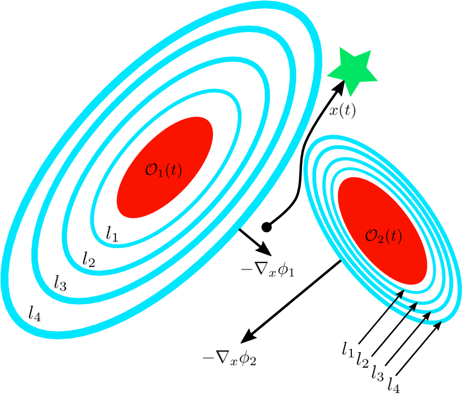
We have then that $H$ defined by (19) solves Problem 1 and is referred to as a C-CBF candidate. Given an arbitrary weight vector $\boldsymbol{w}$, however, it may not be true that $H$ is a valid CBF for (4) with respect to the set $\mathcal{D}(t)$. Without adapting the weights as the system moves through the state space the C-CBF condition (18) may be violated. In what follows we introduce an online parameter adaptation law to enforce (18) and, in doing so, to solve Problem 2.

Consider that in addition to the C-CBF weights $\boldsymbol{w}$ being used to enforce the condition (15), it may be desirable to choose weights that are optimal with respect to some objective function $J:\mathcal{T}\times\R^{c}\times\R^{n}\rightarrow\R$. As such, we propose using a predictor-corrector interior point method for our adaptation law.

Consider the following optimal solution trajectory:

where $J$ is strongly uniformly convex with respect to $\boldsymbol{w}$, twice continuously differentiable in both $\boldsymbol{w}$ and $\boldsymbol{x}$, and piecewise continuously differentiable in $t$. The feasible region is

where the first $c$ constraint functions $b_{j}:\mathcal{T}\times\R^{c}\times\R^{n}\rightarrow\R$ enforce that each $w_{j}$ remains above a user-specified minimum threshold $w_{min}>0$ to ensure that $\boldsymbol{w}(t)\in\R^{c}_{+},\forall t\in\mathcal{T}$, i.e.,

the second $c$ constraint functions $b_{j}:\mathcal{T}\times\R^{c}\times\R^{n}\rightarrow\R$ enforce that each $w_{j}$ remains below a user-specified maximum threshold $w_{max}<\infty$ to ensure that $\boldsymbol{w}(t)$ is well-defined, i.e.,

and the final constraint function $b_{2c+1}:\mathcal{T}\times\R^{c}\times\R^{n}\rightarrow\R$ enforces that the C-CBF condition (15) is satisfied, i.e., namely that

For the moment, let us consider that $b_{2c+1}=\beta$. Recognizing that the optimal solution trajectory (20) is of the form (1), we similarly consider the approximate optimal solution trajectory

where $\Phi$ is analogous to $\Psi$ in (2) and is defined by

for barrier parameter $s>0$. We assume that Assumption 1 holds for $\Phi$ i.e., that there exists $s>0$ rendering $\Phi$ strongly uniformly convex with respect to $\boldsymbol{w}$. As stated previously, this is reasonable in practice given a sufficiently large choice of $s$. We therefore propose to adapt the weights $\boldsymbol{w}$ according to a control-affine dynamical system of the form (3):

where $\mu:\mathcal{T}\times\R^{c}\times\R^{n}\rightarrow\R^{c}$ and $\nu:\mathcal{T}\times\R^{c}\times\R^{n}\rightarrow\R^{c\times m}$ are defined by

for which $\boldsymbol{P}\in\R^{c\times c}$ is a positive-definite gain matrix. Note that $\dot{\boldsymbol{w}}$ given by (27) is affine in $\boldsymbol{u}$ as required in the statement of Problem 2, but, however, that because $\dot{\boldsymbol{w}}$ appears explicitly in (24) (and therefore in (26)) the adaptation law given by (27) with $b_{2c+1}=\beta$ requires solving a partial differential equation (PDE). Rather than attempt to solve this (possibly intractable) PDE, we break the algebraic loop by introducing $\boldsymbol{\mu}^{f}(t)$ and $\boldsymbol{\nu}^{f}(t)$ as filtered versions of $\boldsymbol{\mu}(t)\coloneqq\mu(t,\boldsymbol{w}(t),\boldsymbol{x}(t))$ and $\boldsymbol{\nu}(t)\coloneqq\nu(t,\boldsymbol{w}(t),\boldsymbol{x}(t))$. We assume that these filtered variables track their unfiltered counterparts sufficiently closely, as stated in the following.

The above implicitly define worst-case error bounds $\eta_{\mu}$ and $\eta_{\nu}$ on how the filtered signals $\boldsymbol{\mu}^{f}$ and $\boldsymbol{\nu}^{f}$ affect $\dot{H}$ versus the true signals $\boldsymbol{\mu}$ and $\boldsymbol{\nu}$, and thus the inequality in (24) may be satisfied by using $\boldsymbol{\mu}^{f}$, $\boldsymbol{\nu}^{f}$, $\eta_{\mu}$, and $\eta_{\nu}$ instead of $\boldsymbol{\mu}$ and $\boldsymbol{\nu}$. In practice, (30) and (31) may be satisfied via appropriate filter design. We are now ready to define the final constraint function as

which is directly (24) with the filter variables (and error bounds), specifically

and

with the C-CBF control matrix $\boldsymbol{L}_{g}$ (omitting the dependence on $\boldsymbol{x}$) defined by

and the functions $p_{h}:\R^{c}\times\R^{n}\rightarrow\R^{c}$ and $p_{w}:\R^{c}\times\R^{n}\rightarrow\R^{c}$ given by

These modifications allow us to include $b_{2c+1}$ directly as a function constraining the optimal solution trajectory given by (20) without needing to solve a complicated PDE.

We are now ready to state our main result.

References

- [1] P. Wieland and F. Allgöwer, “Constructive safety using control barrier functions,” IFAC Proceedings Vols., vol. 40, no. 12, pp. 462–467, 2007.
- [2] A. D. Ames, X. Xu, J. W. Grizzle, and P. Tabuada, “Control barrier function based quadratic programs for safety critical systems,” IEEE Trans. on Automatic Control, vol. 62, no. 8, pp. 3861–3876, 2017.
- [3] W. Xiao and C. Belta, “Control barrier functions for systems with high relative degree,” in IEEE 58th Conference on Decision and Control (CDC), 2019, pp. 474–479.
- [4] W. S. Cortez, D. Oetomo, C. Manzie, and P. Choong, “Control barrier functions for mechanical systems: Theory and application to robotic grasping,” in IEEE Trans. on Control Systems Tech., 2019, pp. 1–16.
- [5] Y. Chen, H. Peng, and J. Grizzle, “Obstacle avoidance for low-speed autonomous vehicles with barrier function,” IEEE Transactions on Control Systems Technology, vol. 26, no. 1, pp. 194–206, 2018.
- [6] K. Garg and D. Panagou, “Robust control barrier and control lyapunov functions with fixed-time convergence guarantees,” in 2021 American Control Conference (ACC), 2021, pp. 2292–2297.
- [7] Y. Chen, A. Singletary, and A. D. Ames, “Guaranteed obstacle avoidance for multi-robot operations with limited actuation: A control barrier function approach,” IEEE Control Systems Letters, vol. 5, no. 1, pp. 127–132, 2021.
- [8] M. Jankovic and M. Santillo, “Collision avoidance and liveness of multi-agent systems with cbf-based controllers,” in 2021 60th IEEE Conference on Decision and Control (CDC), 2021, pp. 6822–6828.
- [9] B. Xu and K. Sreenath, “Safe teleoperation of dynamic uavs through control barrier functions,” in 2018 IEEE International Conference on Robotics and Automation (ICRA), 2018, pp. 7848–7855.
- [10] M. Khan, M. Zafar, and A. Chatterjee, “Barrier functions in cascaded controller: Safe quadrotor control,” in 2020 American Control Conference (ACC), 2020, pp. 1737–1742.
- [11] M. Black, M. Jankovic, A. Sharma, and D. Panagou, “Future-focused control barrier functions for autonomous vehicle control,” in 2023 American Control Conference (ACC), to appear, 2023.
- [12] S. Yaghoubi, G. Fainekos, T. Yamaguchi, D. Prokhorov, and B. Hoxha, “Risk-bounded control with kalman filtering and stochastic barrier functions,” in 2021 60th IEEE Conference on Decision and Control (CDC), 2021, pp. 5213–5219.
- [13] L. Wang, D. Han, and M. Egerstedt, “Permissive barrier certificates for safe stabilization using sum-of-squares,” in 2018 Annual American Control Conference (ACC), 2018, pp. 585–590.
- [14] A. Clark, “Verification and synthesis of control barrier functions,” in 60th IEEE Conference on Decision and Control (CDC), 2021, pp. 6105–6112.
- [15] E. Pond and M. Hale, “Fast verification of control barrier functions via linear programming,” arXiv preprint arXiv:2212.00598, 2022.
- [16] J. Breeden and D. Panagou, “High relative degree control barrier functions under input constraints,” in 2021 60th IEEE Conference on Decision and Control (CDC), 2021, pp. 6119–6124.
- [17] W. Xiao, C. Belta, and C. G. Cassandras, “Adaptive control barrier functions,” IEEE Transactions on Automatic Control, vol. 67, no. 5, pp. 2267–2281, 2022.
- [18] K. Garg, E. Arabi, and D. Panagou, “Fixed-time control under spatiotemporal and input constraints: A quadratic programming based approach,” Automatica, vol. 141, p. 110314, 2022.
- [19] K. Garg and D. Panagou, “Control-lyapunov and control-barrier functions based quadratic program for spatio-temporal specifications,” in 58th IEEE Conf. on Decision and Control (CDC), 2019, pp. 1422–1429.
- [20] M. Black, K. Garg, and D. Panagou, “A quadratic program based control synthesis under spatiotemporal constraints and non-vanishing disturbances,” in 2020 59th IEEE Conference on Decision and Control (CDC), 2020, pp. 2726–2731.
- [21] K. Shao, J. Zheng, H. Wang, X. Wang, R. Lu, and Z. Man, “Tracking control of a linear motor positioner based on barrier function adaptive sliding mode,” IEEE Transactions on Industrial Informatics, vol. 17, no. 11, pp. 7479–7488, 2021.
- [22] L. Lindemann and D. V. Dimarogonas, “Control barrier functions for signal temporal logic tasks,” IEEE Control Systems Letters, vol. 3, no. 1, pp. 96–101, 2019.
- [23] G. Yang, C. Belta, and R. Tron, “Continuous-time signal temporal logic planning with control barrier functions,” in 2020 American Control Conference (ACC), 2020, pp. 4612–4618.
- [24] M. Srinivasan and S. Coogan, “Control of mobile robots using barrier functions under temporal logic specifications,” IEEE Transactions on Robotics, vol. 37, no. 2, pp. 363–374, 2021.
- [25] W. S. Cortez, X. Tan, and D. V. Dimarogonas, “A robust, multiple control barrier function framework for input constrained systems,” IEEE Control Systems Letters, vol. 6, pp. 1742–1747, 2022.
- [26] P. Glotfelter, J. Cortes, and M. Egerstedt, “Nonsmooth barrier functions with applications to multi-robot systems,” IEEE Control Systems Letters, vol. 1, pp. 310–315, 10 2017.
- [27] Y. Huang and Y. Chen, “Switched control barrier function with applications to vehicle safety control,” in Dynamic Systems and Control Conference, vol. 84270. American Society of Mechanical Engineers, 2020, p. V001T15A002.
- [28] M. Machida and M. Ichien, “Consensus-based control barrier function for swarm,” in 2021 IEEE International Conference on Robotics and Automation (ICRA), 2021, pp. 8623–8628.
- [29] Z. Cai, H. Cao, W. Lu, L. Zhang, and H. Xiong, “Safe multi-agent reinforcement learning through decentralized multiple control barrier functions,” arXiv preprint arXiv:2103.12553, 2021.
- [30] H. Ma, J. Chen, S. Eben, Z. Lin, Y. Guan, Y. Ren, and S. Zheng, “Model-based constrained reinforcement learning using generalized control barrier function,” in 2021 IEEE/RSJ International Conference on Intelligent Robots and Systems (IROS), 2021, pp. 4552–4559.
- [31] J. Breeden and D. Panagou, “Compositions of multiple control barrier functions under input constraints,” arXiv preprint arXiv:2210.01354, 2022.
- [32] M. Black, E. Arabi, and D. Panagou, “Fixed-time parameter adaptation for safe control synthesis,” arXiv preprint arXiv:2204.10453, 2022.
- [33] B. T. Lopez, J.-J. E. Slotine, and J. P. How, “Robust adaptive control barrier functions: An adaptive and data-driven approach to safety,” IEEE Control Systems Letters, vol. 5, no. 3, pp. 1031–1036, 2021.
- [34] A. J. Taylor and A. D. Ames, “Adaptive safety with control barrier functions,” in 2020 American Control Conference (ACC), 2020, pp. 1399–1405.
- [35] M. Black and D. Panagou, “Adaptation for validation of a consolidated control barrier function based control synthesis,” arXiv preprint arXiv:2209.08170, 2022.
- [36] M. S. Bazaraa, H. D. Sherali, and C. M. Shetty, Nonlinear programming: theory and algorithms. John Wiley & Sons, 2013.
- [37] D. P. Bertsekas, “Convexification procedures and decomposition methods for nonconvex optimization problems,” Journal of Optimization Theory and Applications, vol. 29, no. 2, pp. 169–197, 1979.
- [38] M. Fazlyab, S. Paternain, V. M. Preciado, and A. Ribeiro, “Prediction-correction interior-point method for time-varying convex optimization,” IEEE Trans. on Automatic Control, vol. 63, no. 7, pp. 1973–1986, 2018.
- [39] J. Breeden and D. Panagou, “Robust control barrier functions under high relative degree and input constraints for satellite trajectories,” Automatica, (to be published) 2023.
- [40] Q. Nguyen and K. Sreenath, “Exponential control barrier functions for enforcing high relative-degree safety-critical constraints,” in 2016 American Control Conference (ACC). IEEE, 2016, pp. 322–328.
- [41] M. Jankovic, M. Santillo, and Y. Wang, “Multi-agent systems with cbf-based controllers – collision avoidance and liveness from instability,” arXiv preprint arXiv:2207.04915, 2022.
- [42] W. Xiao, C. A. Belta, and C. G. Cassandras, “Sufficient conditions for feasibility of optimal control problems using control barrier functions,” Automatica, vol. 135, p. 109960, 2022.
- [43] S. Wang, K. Shi, T. Huang et al., “Suboptimal safety-critical control for continuous systems using prediction-correction online optimization,” arXiv preprint arXiv:2203.15305, 2022.
- [44] H. K. Khalil, Nonlinear systems. Prentice hall Upper Saddle River, NJ, 2002, vol. 3.
- [45] R. Rajamani, Vehicle Dynamics and Control. Springer US, 2012.
- [46] W. Xiao and C. Belta, “High-order control barrier functions,” IEEE Transactions on Automatic Control, vol. 67, no. 7, pp. 3655–3662, 2022.
![[Uncaptioned image]](2304.01815v1/Headshot_MitchellBlack.png) |
Mitchell Black (M’20) grew up in Brunswick, Maine, USA. He received his B.S. from Tufts University in 2016 in both Mechanical Engineering and Astrophysics, and his M.S.E. in Aerospace Engineering from the University of Michigan in 2017, where he has been a Ph.D. student in Professor Dimitra Panagou’s Distributed Aerospace Systems and Control Lab since 2020. In the interim (2017-2020), he worked as a Research Scientist at Michigan Aerospace Corporation in Ann Arbor, MI. Mitchell was the 2016 recipient of the National Collegiate Athletic Association’s Walter Byers Postgraduate Scholarship for combined achievement in the classroom and as a member of the Tufts University Track & Field team. He has continued to run throughout graduate school and in 2021 competed at the US Olympic Track & Field Trials in the 800m, where he placed 23rd. |
![[Uncaptioned image]](2304.01815v1/Panagou-v1.png) |
Dimitra Panagou received the Diploma and PhD degrees in Mechanical Engineering from the National Technical University of Athens, Greece, in 2006 and 2012, respectively. In September 2014 she joined the Department of Aerospace Engineering, University of Michigan as an Assistant Professor. Since July 2022 she is an Associate Professor with the newly established Department of Robotics, with a courtesy “dry” appointment with the Department of Aerospace Engineering, University of Michigan. Prior to joining the University of Michigan, she was a postdoctoral research associate with the Coordinated Science Laboratory, University of Illinois, Urbana-Champaign (2012-2014), a visiting research scholar with the GRASP Lab, University of Pennsylvania (June 2013, Fall 2010) and a visiting research scholar with the University of Delaware, Mechanical Engineering Department (Spring 2009). Her research program spans the areas of nonlinear systems and control; multi-agent systems and networks; motion and path planning; human-robot interaction; navigation, guidance, and control of aerospace vehicles. She is particularly interested in the development of provably-correct methods for the safe and secure (resilient) operation of autonomous systems in complex missions, with applications in robot/sensor networks and multi-vehicle systems (ground, marine, aerial, space). She is a recipient of the NASA Early Career Faculty Award, the AFOSR Young Investigator Award, the NSF CAREER Award, and a Senior Member of the IEEE and the AIAA. |