Machine Learning Discovery of Optimal Quadrature Rules for
Isogeometric AnalysisJournal: peer-review
Abstract
We propose the use of machine learning techniques to find optimal quadrature rules for the construction of stiffness and mass matrices in isogeometric analysis (IGA). We initially consider 1D spline spaces of arbitrary degree spanned over uniform and non-uniform knot sequences, and then the generated optimal rules are used for integration over higher-dimensional spaces using tensor product sense. The quadrature rule search is posed as an optimization problem and solved by a machine learning strategy based on gradient-descent. However, since the optimization space is highly non-convex, the success of the search strongly depends on the number of quadrature points and the parameter initialization. Thus, we use a dynamic programming strategy that initializes the parameters from the optimal solution over the spline space with a lower number of knots. With this method, we found optimal quadrature rules for spline spaces when using IGA discretizations with up to 50 uniform elements and polynomial degrees up to 8, showing the generality of the approach in this scenario. For non-uniform partitions, the method also finds an optimal rule in a reasonable number of test cases. We also assess the generated optimal rules in two practical case studies, namely, the eigenvalue problem of the Laplace operator and the eigenfrequency analysis of freeform curved beams, where the latter problem shows the applicability of the method to curved geometries. In particular, the proposed method results in savings with respect to traditional Gaussian integration of up to 44% in 1D, 68% in 2D, and 82% in 3D spaces.
Keywords:
Numerical integration , optimal quadrature rules , machine learning , dynamic programming , isogeometric analysis1 Introduction
Developing efficient and accurate integration methods plays a crucial role in many numerical analysis techniques. In the context of the isogeometric analysis (IGA) [1], a common practical approach for numerical integration is to use an element-wise Gaussian (EWG) quadrature rule when constructing system matrices in the sense of Galerkin discretizations. This follows the classical system construction technique of the finite element analysis (FEA). However, it is known that there exist optimal quadrature rules for spline spaces of higher continuities, thus requiring a significantly fewer number of quadrature points than the classical EWG. For instance, one may consider the fast matrix formation technique by Calabrò et al. 2017, where each row of the system matrices is integrated by its own quadrature rule obtained by a linear system of equations. Bartoň et al. 2020 propose weighted Gaussian quadrature rules for B-splines that require the minimum number of quadrature points while guaranteeing the exactness of integration with respect to the weight function. Other techniques by Bartoň and Calo 2016a, Bartoň and Calo 2016b, Bartoň and Calo 2017 use a polynomial homotopy continuation (PHC), a numerical scheme for solving polynomial systems of equations [7], to generate Gaussian quadrature rules for spline spaces of higher continuities. To generate a Gaussian rule in a target spline space, they built an associated source space with known quadratures (e.g., a union of polynomial Gaussian rules) and transform the rule from the source space to the target space, while preserving the optimality. These rules, in the limit (when the number of elements are very large), converge to the half-point rules of Hughes et al. 2010. More research works on obtaining optimal or nearly optimal quadrature rules for IGA discretizations can be found in, e.g., [9, 10, 11, 12, 13, 14].
On the other hand, the use of machine learning techniques to address numerical integration problems is gaining momentum in recent years. While the practical state-of-the-art for calculating approximate integrals with bounded errors are still Monte Carlo methods [15], kernel-based quadrature approaches have proved interesting convergence properties, making them suitable for high-dimensional problems, or when the integrand function is expensive to evaluate [16, 17]. Another example are Bayesian quadrature methods [18, 19, 20], which aim at providing a statistically accurate integration while minimizing the required number of evaluations of the integrand. Quadrature techniques are also a relevant stage on deep learning-based approximations, for which no proper rules exist (see, e.g., [21]). All of the mentioned approaches try to calculate an approximate value of the integral, while the main contribution of this work lies in providing optimal quadrature rules, in the sense of calculating the exact integral with the minimum possible number of quadrature points.
In order to guarantee the optimality of the discovered rules, we first define the target number of quadrature points according to the half-point rule [8], and then set as trainable parameters the location and weight of each point. The loss function that completes the definition of the machine learning problem is based on the integration error of each individual basis function in the fixed finite dimensional spline space. However, this problem is highly non-convex, and the convergence of the learning process to the global optimum depends fundamentally on the initial value of the parameters [22]. For this reason, and exploiting the regularity of spline spaces with the same degree and continuity, but different numbers of elements, we devise a dynamic programming strategy [23] that initializes the parameters of a given problem from the optimal solution of a simpler problem. The experimental results show that this strategy achieves general convergence on partitions with uniform elements.
The structure of the remainder of this paper is as follows: Section 2 formally defines the target function spaces and the integration problem. In Section 3, we describe the developed optimization method, including the loss function and a dynamic programming strategy for parameter initialization. Then, Section 4 shows the numerical results of the obtained quadrature rules for general spline spaces, their comparison with classical EWG rules, and the computational requirements. In Section 5, we discuss the IGA results of two applied case studies. Finally, Section 6 draws some conclusions and indicates possible directions for future research.
2 Problem formulation
2.1 IGA discretization
For the sake of simplicity, we consider an IGA discretization over the one-dimensional parameter space. The extension to the higher-dimensional spaces is trivial by taking tensor products. Without loss of generality, we introduce the computational domain as a partition of elements in , described by a sequence of non-repeating knots such that . We define the B-spline space of piecewise polynomial functions of degree with continuity at every interior knot in , where . Let us consider the clamped knot vector as
| (2.1) |
where is the multiplicity of interior knots and is the dimension of . We obtain the basis functions of this B-spline space by the Cox–De Boor recursion [24]. For a given parameter , it reads
| (2.2) | ||||
| (2.3) |
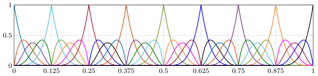
When evaluating basis functions at a desired , we find the corresponding nonzero knot span in (2.2) and efficiently evaluate (2.3) avoiding any division by zero in dealing with repetitive knots. More details are given in [24, Algorithms A2.1 and A2.2] and [25, Algorithms A1 and A2]. Fig. 1 shows an example of B-spline bases characterized by and spanned over a uniform partition with elements.
Remark 1.
We note that admits different basis functions. For example, an alternative set of bases are and . However, they produce excessively large condition numbers that lead to numerical instabilities when searching for the optimal quadrature rules.
2.2 Numerical integration
Without loss of generality, we aim at finding optimal quadrature rules to exactly compute the following integrals when constructing the stiffness and mass matrices arising from the discretization of a partial differential equation (PDE):
| (2.4) | ||||||
| (2.5) |
where the prime denotes the derivative of the basis functions. For the sake of brevity, herein and in the following, we omit the superscript in referring to basis functions. We note that the integrals (2.4) and (2.5) are formed without taking into account the coefficients of the investigated PDE and the problem geometry. This is a common assumption when seeking to compute the optimal quadrature rules (see, e.g., [8, Section 3.2] and [9, Section 2]).
Remark 2.
Let be a spline space used for IGA discretization, the product of basis function derivatives in (2.4) entails integrating the space , while in (2.5), we integrate the space . As a result, the minimal space that contains both stiffness and mass terms is . Furthermore, when using typical maximum-continuity IGA discretizations, is equal to . Thus, for brevity, we consider the space for the integrand, where is equal to , and is up to .
We wish to find quadrature points and weights presuming that a given integral bilinear form is evaluated exactly on . Thus, for any , we have
| (2.6) |
We note, however, that it suffices to produce an appropriate quadrature rule in a larger space for integrals, as we have that if , then in the sense of Remark 2. Thus, we aim to find quadrature rules for integration of the form
| (2.7) |
for all , with the following constraints:
| (2.8) | ||||
When constructing system matrices in IGA, a common practical approach is to use the classical element-wise Gaussian (EWG) quadrature rule that entails a -point rule within each element , , for integrals (2.4) and (2.5). This element-wise rule is optimal only when using a discontinuous space (i.e., with continuity at all elements interfaces), which could be the case in the classical FEA discretizations. Thus, the extra cost of EWG rules in IGA may lead to significant computational overheads, particularly with higher-order discretizations and in higher-dimensional problems. For spline spaces, there always exists an optimal quadrature rule where the number of quadrature points is given by:
| (2.9) |
where is the total number of interior knots, including their multiplicities, i.e., assuming a uniform continuity at all interior knots. If , then , denoting that in the limit, when , the mentioned spline rules converge to the half-point rules of Hughes et al. 2010, which are exact over the domain. Therefore, we consider a quadrature rule to be optimal if is the minimum required number of quadrature points, while guaranteeing the exactness of the integration.
Remark 3.
Based on some combinations of , , and , the left-hand side in (2.9) may become odd; thus, we obtain the optimal number of quadrature points by . In such occasions, one may consider a higher space to have a unique quadrature rule following the idea of integrating over odd-degree spline spaces described in, e.g., [5]. However, this implies the over-integration of system matrices.
3 Optimization method
3.1 Parameter space and loss function
As is a finite-dimensional space, all norms upon it are equivalent, and we consider it to be equipped with the norm. Then, for each fixed , we can view as a linear functional on . In this case, the natural way to quantify the integration error would be using the dual norm defined over . Whilst dual norms are generally difficult to evaluate, as we consider to be the norm on , we have a straightforward numerically tractable expression for the induced dual norm. Specifically, if is the exact integral of , we have
| (3.1) |
Given any basis of , we consider the Gram (a.k.a mass) matrix given by (2.5) and, by utilizing the Hilbert space structure of and its dual space, we define our loss function as:
| (3.2) |
where is the integration error for the basis function, that is for a fixed and :
| (3.3) |
If the basis were orthonormal, then and its inverse would be the identity matrix, and generally is utilized to ensure consistency between the loss and the norm within a general basis.
In general, for a fixed number of quadrature points , there are unknown parameters corresponding to the point locations and weights , and the optimization problem consists of minimizing while respecting the constraints defined in (2.8). Since (3.2) is differentiable, we approach this problem first by setting the optimal number of points to calculate as , c.f. [8], and then by using a standard machine learning strategy based on gradient-descent. However, we observe that the optimization space is highly non-convex, and thus the search usually stagnates at local minima, being highly dependent on and the initial values of and . This is illustrated in Fig. 2, where we show the optimization space for a simple problem (, and ). In this space, is equal to three; but due to the symmetry constraints explained below (3.4), together with the basic constraints in (2.8), the loss is determined by and only. We can see that even in this simple space there are multiple local minima, and the ability of gradient descent to effectively find the solution depends on the starting point for searching.


3.2 Dynamic programming for parameter initialization
Given the relevance of the initial values of the searching parameters for the convergence of the machine learning optimization, we devise a method based on dynamic programming [23] to initialize the parameter values in a fully deterministic way. In short, the initial parameter values for a given problem will be calculated from the optimal quadrature rule of a simpler problem. This allows us to break the solution of a problem into a chain of simpler problems and to solve it recursively. Let us start by discussing how to solve problems with uniform elements, and then, we will build on those results to address more general problems with non-uniform elements.
3.2.1 Uniform elements
We consider a partition to be uniform if the distance between any two consecutive non-repeating knots and , , is constant. In these cases, due to symmetry in the function space around the center, we can impose two additional constraints to our optimal quadrature rule:
| (3.4) | ||||
Thus, the number of parameters to fit is points and weights. Then, given a space , for , the parameter initialization will be done as follows:
| (3.5) | ||||
| (3.6) |
where and are the optimal quadrature points and weights for the space . That is, the initial values when searching for a solution in a partition with elements result from a linear scaling of the optimal solution for a partition with elements. The base case is , in which the initial values for are uniformly distributed in the interval , and all the weights are . This procedure is illustrated in Fig. 3. Even if the number of optimal quadrature points increases with the number of elements (for fixed and ), it holds that , and therefore this procedure can always be applied.
For zero-continuity spaces (i.e., ), a better initialization is achieved as follows:
| (3.7) | ||||
| (3.8) |
The main advantage in this case is that the initialization does not depend on a quadrature rule for a different space, and therefore we can directly run the optimization for an arbitrary number of elements without having to solve the problem for fewer elements.
3.2.2 Non-uniform elements
When our element domain forms a non-uniform partition, we cannot exploit the constraints in (3.4) to reduce the number of optimization parameters because the symmetry of the function space around the center no longer holds. In such occasions, we initialize the values of and from the optimal rule for a space with a uniform partition and the same , and . Thus, given a space with a non-uniform partition (i.e., is not constant), and the corresponding space with a uniform partition and its optimal quadrature rule as , , we calculate the initial parameter values for every as follows:
| (3.9) | ||||
| (3.10) |
Basically, we calculate a length scale given by for each element with respect to the uniform partition, and then linearly apply this scale to the optimal points and weights belonging to that element. Fig. 4 visually shows an example for a space with a random non-uniform partition of 8 elements.
3.3 Optimization loop
Once the initial values are set, we start a regular gradient-descent search using the Yogi optimizer [26]. The only parameter of the optimizer that has to be tuned is the learning rate. We notice that this tuning should be driven by the complexity of the problem represented by , since the larger the number of parameters, the more sensitive the loss function is to small numeric variations, affecting the smoothness of the search space. We also observed that with just an inverse linear scaling, the search occasionally stalls by jumping around the solution, and thus we opt for an inverse log-linear scaling by setting the learning rate as .
On the other hand, since an exact solution is difficult to find in practice through a gradient-descent approach (due to floating-point arithmetic), we consider a quadrature rule to be optimal if . The search stops if either or we reach the limit of 10,000 gradient-descent iterations (a.k.a epochs).
4 Numerical results
4.1 Implementation details
The proposed method has been fully implemented in the Python programming language, relying heavily on the JAX [27] and Optax [28] libraries. All the experiments have been performed in a laptop PC with an Intel(R) Core(TM) i7-1250U CPU, 32 GB of RAM memory and a Linux kernel v5.19. The version of Python in which we ran the experiments was 3.10.
With the aim of supporting reproducible research, the full source code required to reproduce the experimental results described below is provided as open-source software. We also provide a table with the optimal quadrature rules in double precision for spaces up to and arbitrary with uniform partitions of up to elements. All this may be downloaded from https://gitlab.bcamath.org/tteijeiro/spline-integration
4.2 General experiments
The first experiments aim at evaluating the generality of the proposed method, both with uniform and non-uniform partitions. For this, we performed an exhaustive search of optimal quadrature rules for spline spaces with all combinations of and uniform partitions with , corresponding to 6664 cases. For all cases, we succeed in obtaining optimality, so that . Fig. 5 shows the distribution of the number of epochs required to converge to the optimal rule based on the number of elements. Even if the difficulty clearly increases with the number of elements, the scalability shown by the method is really positive, with a global median of 522 required epochs per rule, and with 90% of the rules requiring less than 1700 epochs to meet the stopping criteria of . It is also interesting to see the case of in which the recursive parameter initialization is not applied and the number of required epochs is generally higher, thus indicating the advantage of the proposed initialization technique.
To test the method on non-uniform partitions, we randomly generate 3000 function spaces with the following values of : , and with a variable number of elements . For each combination of , we generate 100 independent partitions by randomly sampling and sorting values from a uniform distribution in the interval . Then, for each of these 3000 function spaces, we initialize and optimize the parameters and according to the method described in Sections 3.2.2 and 3.3. Unlike with uniform partitions, in this case the optimization loop did not converge to an optimal quadrature rule in 100% of the cases. Fig. 6 shows the results for different number of elements. 6(a) depicts the distributions in the number of epochs, which are in general much higher than uniform partitions. Additionally, more than 50% of the spaces reach the limit of 10000 epochs. 6(b) shows the percentage of partitions for which the method was able to find an optimal rule, that is , according to the number of elements. The reduction in the success rate is fundamentally linear, and thus the method cannot be considered of general applicability for . In future work we will focus on characterizing additional constraints that must be satisfied by the partition knots to improve the convergence.
4.3 Computational requirements
To evaluate the computational demands of our method, we assess the time required to find a quadrature rule with respect to the complexity of the rule, measured as the number of quadrature points to optimize () and considering only uniform partitions. However, is determined by the spline space, and there might be two different spaces leading to the same . Thus, we will separately assess the influence of , , and to get a better overview of how the method scales in practice. Fig. 7 shows three graphs of the time required to calculate rules for increasing values of . In 7(a), the number of points increases by increasing the maximum degree of the space , while keeping a fixed number of elements and a fixed continuity for each plotted line. On the other hand, in 7(b) the value of increases by decreasing , keeping the same and a fixed for each line. Finally, 7(c) keeps a fixed degree and continuity for each line, and increases between 4 and 50 to increase . All charts are in logarithmic scale on the time axis.
We can see that, in general, the time requirements grow exponentially with the number of parameters. Still, this growth is much faster when the reason is the complexity of the function space (higher degree or lower continuity) than the case where the reason is an increased number of elements. Indeed, we can observe that for a space with and , the increase is basically linear, and this is due to the fact that, in this space, the initialization method described in Section 3.2.1 already gives an optimal rule, not requiring any gradient descent iterations. From a practical point of view, we can see that the quadrature rule for a realistic space with , and can be calculated in approximately 1 second, while an overly complex space with , and can take up to 36 seconds. We want to reiterate that these experiments were performed in a common laptop CPU, so these times could be significantly reduced by using a more powerful hardware.
4.4 Optimal vs. element-wise Gaussian rules
Herein, we compare the computational cost of numerical integration when using the optimal and classical EWG quadrature rules. For this purpose, we consider the total number of required quadrature points in 1D, 2D, and 3D parameter spaces when constructing the mass and stiffness matrices in the sense of IGA discretization. For 2D and 3D spaces, when the coefficients of the desired PDE are constant along different spatial directions, one may construct the system matrices in 1D and then obtain the matrices in higher dimensions through the tensor product of 1D matrices (see, e.g., [29, 30]). In this case, the cost of numerical integration in higher dimensions is equal to that of 1D spaces. However, when the coefficients are varying through the domain in different directions, which could be the case in problems arising in electromagnetics and geoscience (see, e.g., [31, 32]), we construct the system matrices by integrating higher-dimensional basis functions. Thus, the required number of quadrature points (i.e., the integration cost) grows by the power of the dimension space and the advantage of using the proposed optimal quadrature rules is more tangible. Table 1 shows the specific savings for some relevant spaces in different dimensions when using functions in as the integrand in the sense of Remark 2. The improvements for all tested values of and are illustrated in Fig. 8.
| Dimensionality | Degree | Number of elements | Number of quadrature points | Relative savings when using optimal rules | |
| EWG rule | Optimal rule | ||||
| 1D | 2 | 20 | 60 | 41 | 31.7% |
| 50 | 150 | 101 | 32.7% | ||
| 4 | 20 | 100 | 62 | 38.0% | |
| 50 | 250 | 152 | 39.2% | ||
| 8 | 20 | 180 | 104 | 42.2% | |
| 50 | 450 | 254 | 43.6% | ||
| 2D | 2 | 20 | 3,600 | 1,681 | 53.3% |
| 50 | 22,500 | 10,201 | 54.7% | ||
| 4 | 20 | 10,000 | 3,844 | 61.6% | |
| 50 | 62,500 | 23,104 | 63.0% | ||
| 8 | 20 | 32,400 | 10,816 | 66.7% | |
| 50 | 202,500 | 64,516 | 68.1% | ||
| 3D | 2 | 20 | 216,000 | 68,921 | 68.1% |
| 50 | 3,375,000 | 1,030,301 | 69.5% | ||
| 4 | 20 | 1,000,000 | 238,328 | 76.2% | |
| 50 | 15,625,000 | 3,511,808 | 77.5% | ||
| 8 | 20 | 5,832,000 | 1,124,864 | 80.7% | |
| 50 | 91,125,000 | 16,387,064 | 82.0% | ||
5 Case studies
To study the accuracy of the proposed optimal quadrature rules on spline spaces, we consider two case studies, namely, the eigenproblem of the Laplace operator and the eigenfrequency analysis of a curved beam.
5.1 Eigenvalue problem of the Laplace operator
We consider the eigenproblem of the Laplace operator in 1D. Given as our computational domain with boundary , we write
| (5.1) |
Let us consider gradient-conforming functional space. We define the Sobolev space of functions in that are vanishing on the boundary. Taking as an arbitrary test function, we build the weak form of (5.1) as follows: Find and , such that for all ,
| (5.2) |
where
| (5.3) | ||||
| (5.4) |
Then, by employing an IGA discretization spanned by over the knot sequence with bases , we define the discrete space . Thus, we obtain the discrete eigenproblem: Find and , such that for all ,
| (5.5) |
where and refer to approximated eigenpairs. Equation (5.5) leads to the following generalized eigenproblem in the matrix form:
| (5.6) |
where denotes the eigenvectors. We obtain the stiffness and mass matrices, and , respectively, using integrals (2.4) and (2.5). In the following, we consider the eigensolution of (5.6) when constructing the system matrices using both the proposed optimal and the classical element-wise Gaussian quadrature rules. For the former, we create our rules based on the spline space as the integrand (c.f. Remark 2). In all tests, we show that the optimal quadrature rules have the same order of exactness as the classical EWG rules while constructing matrices with lower computational efforts (see Section 4.4).
5.1.1 Uniform domain
We first consider IGA discretizations with uniform elements and basis functions of polynomial degrees . For every eigenpair, we introduce the eigenvalue error
| (5.7) |
where , , are the analytical eigenvalues, being the total number of degrees of freedom (equal to in this 1D test case). Fig. 9 shows, in logarithmic scale, the eigenvalue error against the normalized mode number when solving (5.6) in a domain with uniform elements. The results show that the spectral approximation obtained by both optimal and EWG rules are identical even in the high-frequency region where the outlier effect deteriorates the quality of the approximation. Since the domain consists of uniform elements, the theoretical convergence rate of is conserved (c.f. [30]).
5.1.2 Uniform domain with a fine mesh
In the next test, we consider finer domains (i.e., with higher number of elements) for which we do not construct any optimal rule. Dealing with fine meshes is a common practice in FEA and IGA when we seek lower approximation errors. In such occasions, we consider one optimal rule from those described in Section 4.2. Then, we subdivide our domain into blocks of macroelements in such a way that the number of elements at each block is equal to the number of elements for which we have the optimal rule. This follows the terminology of the refined isogeometric analysis (rIGA) [33], where we introduce zero-continuity basis functions to split the domain into macroelements. Since the system matrices at each block are constructed separately, we exploit the advantage of using the optimal rules for any given fine mesh with elements. Furthermore, using separators in the mesh helps to reduce the interconnection between degrees of freedom, thus, reducing the solution costs when employing direct solvers for matrix factorization (c.f. [33, 29] for more details). Fig. 10 depicts an example set of cubic basis functions in a domain with elements, that is subdivided into four blocks each containing 16 elements.
To assess how the employment of the rIGA framework affects the results, we consider a uniformly-spaced 128-element domain and investigate the eigensolution accuracy of the eigenproblem of the Laplace operator. Fig. 11 shows the eigenvalue errors against the normalized mode number . We note that an rIGA-discretized system has more degrees of freedom compared to its IGA counterpart. This is because the continuity reduction at separators increases the dimension of the spline space. Thus, to have a true comparison with an IGA-discretized system constructed by EWG quadrature rules, we consider for mode number normalization. Herein, we consider blocks with 16 element and polynomial degrees . The accuracy of the eigensolution for the lower-frequency part of the spectra are identical when using optimal and EWG rules. However, the high-frequency region shows slightly better spectral approximations, particularly for higher degrees, when incorporating the optimal rules into the IGA framework. This improvement is mainly due to the effect that rIGA has on the spectral approximation (see, e.g., [29, 34] for more details).
5.1.3 Non-uniform domain
As a final test, we consider non-uniform elements in the IGA discretization of the eigenproblem (5.1). Let us consider a domain with 20 non-uniform elements (for which our optimization is converged properly to optimal rules). In particular, we consider the solution over the following unevenly-spaced knot sequence:
| (5.8) |
Fig. 12shows the eigenvalue errors considering as the polynomial degree of basis functions. Again, the accuracy of the spectral approximation is identical when using either of the optimal or EWG rules for system construction. However, it is clear that the eigenvalue error plots deviate from the theoretical convergence rates due to the non-uniformity of the domain.
5.2 Eigenfrequency analysis of the Tschirnhausen beam, a curved geometry
In the second case study, we investigate the performance of the proposed optimal quadrature rules when integrating over a curved geometry. For this purpose, we consider the eigenfrequency analysis of the Tschirnhausen beam characterized by a planar freeform geometry with varying curvature.
5.2.1 Geometry representation
Given the parametric domain , we represent the geometry of the beam midline by a B-spline curve with control points , . For any parameter and B-spline bases given by (2.3), it reads
| (5.9) |
Let us consider quadratic bases (i.e., ) spanned over the knot vector . Fig. 13 shows the midline of the Tschirnhausen beam and its corresponding control points listed in Table 2. We use the algebraic formula of the Tschirnhausen curve (see, e.g., [35, 36]) and, then, generate the control points by a curve fitting process [24].
| Control points | |||||||
|---|---|---|---|---|---|---|---|
| -component | 0.0000 | 0.0122 | 0.2121 | 0.4196 | 0.6208 | 0.8099 | 0.9000 |
| -component | 0.0000 | 0.1137 | 0.2065 | 0.1945 | 0.1385 | 0.0519 | 0.0000 |
5.2.2 Eigenfrequency analysis
We use the Timoshenko curved beams formulation; but details are omitted for the sake of brevity (see, e.g., [37, 38] for complete formulation). In this context, each nodal component of the beam has three degrees of freedom, namely, tangential and normal displacements of the midline, and , respectively, and transverse rotation of the cross section . We assume our computational domain as a mapping from the rectilinear parameter domain onto the curved geometry. Let us introduce with as the vector of degrees of freedom, and as our test space. We write the eigenproblem associated with the frequency analysis of curved beams in the weak form as follows: Find and , such that for all ,
| (5.10) |
where is the eigenfrequency. We define the bilinear forms
| (5.11) | ||||
| (5.12) |
with
| (5.13) | ||||
| (5.14) | ||||
| (5.15) |
where is the curvature of the midline, is the material density, and are the elastic and shear modulus of the material of the beam, is cross-section area, is the second moment of inertia of cross-section, and is the shear correction factor.
In the IGA framework, it is a common practice to use the same basis functions that define the geometry to discretize the solution fields , , and . Let us introduce as our discrete spaces in the parametric domain. We define the discrete space in the physical domain
| (5.16) |
where is the pullback mapping to the parameter space (see, e.g., [31]). Thus, we write the discrete form of the eigenproblem (5.10) as follows: Find and , such that for all ,
| (5.17) |
that results in the same matrix form as (5.6), while the total number of degrees of freedom is increased to . When constructing the stiffness and mass matrices given by the bilinear forms (5.11) and (5.12), we integrate over the curved domain noting that the derivatives in (5.13) are also expressed in the curvilinear coordinate system. Let
| (5.18) |
be the Jacobian, which is the Euclidean norm of the derivative of the geometry, we write and to compute the derivatives and integrals in the rectilinear parameter domain . In this notation, we compute the curvature of the geometry as follows:
| (5.19) |
In the following, we compare the eigenvalue errors of the Tschirnhausen curved beam when constructing the system matrices using the optimal and EWG quadrature rules (see Fig. 14). We consider uniform elements and polynomial degrees to discretize the respective eigenproblem. The difference between results of the optimal and EWG rules is because of the variation of the curvature and the inclusion of the geometric terms in integrals (5.11) and (5.12). Nevertheless, neither of these rules are exact in this case because they are constructed based on (2.4) and (2.5) without taking into account the geometric terms in the integration (c.f. [8, Section 3.2] and [9, Section 2]). Finally, we note that the low-frequency region of the spectrum of this curved beam shows relatively high frequency errors under the employment of typical IGA discretizations (see, e.g., [36, 39]).
6 Conclusions
We have developed and validated a novel machine-learning method for finding optimal quadrature rules on B-spline spaces. This method has shown general convergence to the optimal rule on uniform elements with arbitrary degrees and continuities, with a good computational scalability. We have also employed the method to construct system matrices for practical IGA problems to assess its accuracy. In particular, we solved the eigenproblem of the Laplace operator and eigenfrequency problem of a planar curved beam. We showed that the results are equivalent to element-wise Gaussian integration, but requiring up to 44% fewer integration points. These savings are magnified when performing integrals over high-dimensional basis functions, reaching 68% in 2D spaces, and up to 82% in 3D spaces. Finally, even if we have demonstrated that the method works for some partitions with non-uniform elements, as a future line of research we will pursue a strategy that is generally applicable in this scenario.
Acknowledgements
This work has been funded by the Euskampus Foundation through the ORLEG-IA project in the Misiones Euskampus 2.0 program, the “BCAM Severo Ochoa” accreditation of excellence CEX2021-001142-S / MICIN / AEI / 10.13039/501100011033, the projects of the Spanish Ministry of Science and Innovation PID2019-108111RB-I00, PDC2021-121093-I00, TED2021-132783B-I00, and the Basque Government through the BERC 2022-2025 program and the Consolidated Research Group MATHMODE (IT1456-22) given by the Department of Education. T. Teijeiro is supported by the grant RYC2021-032853-I funded by MCIN/AEI/ 10.13039/501100011033 and by the EU NextGenerationEU/PRTR.
References
- Hughes et al. [2005] T. J. R. Hughes, J. A. Cottrell, Y. Bazilevs, Isogeometric analysis: CAD, finite elements, NURBS, exact geometry and mesh refinement, Computer Methods in Applied Mechanics and Engineering 194 (2005) 4135–4195. doi:10.1016/j.cma.2004.10.008.
- Calabrò et al. [2017] F. Calabrò, G. Sangalli, M. Tani, Fast formation of isogeometric Galerkin matrices by weighted quadrature, Computer Methods in Applied Mechanics and Engineering 316 (2017) 606–622. doi:10.1016/j.cma.2016.09.013.
- Bartoň et al. [2020] M. Bartoň, V. Puzyrev, Q. Deng, V. Calo, Efficient mass and stiffness matrix assembly via weighted Gaussian quadrature rules for B-splines, Journal of Computational and Applied Mathematics 371 (2020) 112626. doi:10.1016/j.cam.2019.112626.
- Bartoň and Calo [2016a] M. Bartoň, V. M. Calo, Gaussian quadrature for splines via homotopy continuation: Rules for cubic splines, Journal of Computational and Applied Mathematics 296 (2016a) 709–723. doi:10.1016/j.cam.2015.09.036.
- Bartoň and Calo [2016b] M. Bartoň, V. M. Calo, Optimal quadrature rules for odd-degree spline spaces and their application to tensor-product-based isogeometric analysis, Computer Methods in Applied Mechanics and Engineering 305 (2016b) 217–240. doi:10.1016/j.cma.2016.02.034.
- Bartoň and Calo [2017] M. Bartoň, V. M. Calo, Gauss–Galerkin quadrature rules for quadratic and cubic spline spaces and their application to isogeometric analysis, Computer-Aided Design 82 (2017) 57–67. doi:10.1016/j.cad.2016.07.003.
- Sommese and Wampler [2005] A. J. Sommese, C. W. Wampler, The Numerical Solution of Systems of Polynomials Arising in Engineering and Science, World Scientific, Singapore, 2005.
- Hughes et al. [2010] T. J. R. Hughes, A. Reali, G. Sangalli, Efficient quadrature for NURBS-based isogeometric analysis, Computer Methods in Applied Mechanics and Engineering 199 (2010) 301–313. doi:10.1016/j.cma.2008.12.004.
- Auricchio et al. [2012] F. Auricchio, F. Calabrò, T. J. R. Hughes, A. Reali, G. Sangalli, A simple algorithm for obtaining nearly optimal quadrature rules for NURBS-based isogeometric analysis, Computer Methods in Applied Mechanics and Engineering 249-252 (2012) 15–27. doi:10.1016/j.cma.2012.04.014.
- Schillinger et al. [2014] D. Schillinger, S. J. Hossain, T. J. R. Hughes, Reduced bézier element quadrature rules for quadratic and cubic splines in isogeometric analysis, Computer Methods in Applied Mechanics and Engineering 277 (2014) 1–45. doi:10.1016/j.cma.2014.04.008.
- Hiemstra et al. [2017] R. R. Hiemstra, F. Calabrò, D. Schillinger, T. J. R. Hughes, Optimal and reduced quadrature rules for tensor product and hierarchically refined splines in isogeometric analysis, Computer Methods in Applied Mechanics and Engineering 316 (2017) 966–1004. doi:10.1016/j.cma.2016.10.049.
- Barendrecht et al. [2018] P. J. Barendrecht, M. Bartoň, J. Kosinka, Efficient quadrature rules for subdivision surfaces in isogeometric analysis, Computer Methods in Applied Mechanics and Engineering 340 (2018) 1–23. doi:10.1016/j.cma.2018.05.017.
- Zou et al. [2021] Z. Zou, T. J. R. Hughes, M. A. Scott, R. A. Sauer, E. J. Savitha, Galerkin formulations of isogeometric shell analysis: Alleviating locking with Greville quadratures and higher-order elements, Computer Methods in Applied Mechanics and Engineering 380 (2021) 113757. doi:10.1016/j.cma.2021.113757.
- Giannelli et al. [2022] C. Giannelli, T. Kanduč, M. Martinelli, G. Sangalli, M. Tani, Weighted quadrature for hierarchical B-splines, Computer Methods in Applied Mechanics and Engineering 400 (2022) 115465. doi:10.1016/j.cma.2022.115465.
- Mon [2004] Monte Carlo integration I, in: Physically Based Rendering, Elsevier, 2004, pp. 631–660. doi:10.1016/B978-012553180-1/50016-8.
- Kanagawa et al. [2016] M. Kanagawa, B. K. Sriperumbudur, K. Fukumizu, Convergence guarantees for kernel-based quadrature rules in misspecified settings, in: D. Lee, M. Sugiyama, U. Luxburg, I. Guyon, R. Garnett (Eds.), Advances in Neural Information Processing Systems, volume 29, Curran Associates, Inc., 2016. doi:10.5555/3157382.3157466.
- Munkhoeva et al. [2018] M. Munkhoeva, Y. Kapushev, E. Burnaev, I. Oseledets, Quadrature-based features for kernel approximation, in: S. Bengio, H. Wallach, H. Larochelle, K. Grauman, N. Cesa-Bianchi, R. Garnett (Eds.), Advances in Neural Information Processing Systems, volume 31, Curran Associates, Inc., 2018. doi:10.5555/3327546.3327589.
- O’Hagan [1991] A. O’Hagan, Bayes–Hermite quadrature, Journal of Statistical Planning and Inference 29 (1991) 245–260. doi:10.1016/0378-3758(91)90002-V.
- Karvonen and Sarkka [2017] T. Karvonen, S. Sarkka, Classical quadrature rules via Gaussian processes, in: 2017 IEEE 27th International Workshop on Machine Learning for Signal Processing (MLSP), IEEE, Tokyo, 2017, pp. 1–6. doi:10.1109/MLSP.2017.8168195.
- Kanagawa and Hennig [2019] M. Kanagawa, P. Hennig, Convergence guarantees for adaptive bayesian quadrature methods, in: H. Wallach, H. Larochelle, A. Beygelzimer, F. d'Alché-Buc, E. Fox, R. Garnett (Eds.), Advances in Neural Information Processing Systems, volume 32, Curran Associates, Inc., 2019. doi:10.5555/3454287.3454847.
- Rivera et al. [2022] J. A. Rivera, J. M. Taylor, Á. J. Omella, D. Pardo, On quadrature rules for solving Partial Differential Equations using Neural Networks, Computer Methods in Applied Mechanics and Engineering 393 (2022) 114710. doi:10.1016/j.cma.2022.114710.
- Narkhede et al. [2022] M. V. Narkhede, P. P. Bartakke, M. S. Sutaone, A review on weight initialization strategies for neural networks, Artificial Intelligence Review 55 (2022) 291–322. doi:10.1007/s10462-021-10033-z.
- Bellman [1966] R. Bellman, Dynamic Programming, Science 153 (1966) 34–37. doi:10.1126/science.153.3731.34.
- Piegl and Tiller [1996] L. Piegl, W. Tiller, The NURBS book, Springer-Verlag, 1996.
- Hashemian et al. [2022] A. Hashemian, D. Garcia, D. Pardo, V. M. Calo, Refined isogeometric analysis of quadratic eigenvalue problems, Computer Methods in Applied Mechanics and Engineering 399 (2022) 115327. doi:10.1016/j.cma.2022.115327.
- Zaheer et al. [2018] M. Zaheer, S. Reddi, D. Sachan, S. Kale, S. Kumar, Adaptive methods for nonconvex optimization, in: S. Bengio, H. Wallach, H. Larochelle, K. Grauman, N. Cesa-Bianchi, R. Garnett (Eds.), Advances in Neural Information Processing Systems, volume 31, Curran Associates, Inc., 2018.
- Bradbury et al. [2018] J. Bradbury, R. Frostig, P. Hawkins, M. J. Johnson, C. Leary, D. Maclaurin, G. Necula, A. Paszke, J. VanderPlas, S. Wanderman-Milne, Q. Zhang, JAX: composable transformations of Python+NumPy programs, 2018. URL: http://github.com/google/jax.
- Babuschkin et al. [2020] I. Babuschkin, K. Baumli, A. Bell, S. Bhupatiraju, J. Bruce, P. Buchlovsky, D. Budden, T. Cai, A. Clark, I. Danihelka, A. Dedieu, C. Fantacci, J. Godwin, C. Jones, R. Hemsley, T. Hennigan, M. Hessel, S. Hou, S. Kapturowski, T. Keck, I. Kemaev, M. King, M. Kunesch, L. Martens, H. Merzic, V. Mikulik, T. Norman, G. Papamakarios, J. Quan, R. Ring, F. Ruiz, A. Sanchez, R. Schneider, E. Sezener, S. Spencer, S. Srinivasan, W. Stokowiec, L. Wang, G. Zhou, F. Viola, The DeepMind JAX Ecosystem, 2020. URL: http://github.com/deepmind.
- Hashemian et al. [2021] A. Hashemian, D. Pardo, V. M. Calo, Refined isogeometric analysis for generalized Hermitian eigenproblems, Computer Methods in Applied Mechanics and Engineering 381 (2021) 113823. doi:10.1016/j.cma.2021.113823.
- Puzyrev et al. [2017] V. Puzyrev, Q. Deng, V. Calo, Dispersion-optimized quadrature rules for isogeometric analysis: Modified inner products, their dispersion properties, and optimally blended schemes, Computer Methods in Applied Mechanics and Engineering 320 (2017) 421–443. doi:10.1016/j.cma.2017.03.029.
- Garcia et al. [2019] D. Garcia, D. Pardo, V. M. Calo, Refined isogeometric analysis for fluid mechanics and electromagnetics, Computer Methods in Applied Mechanics and Engineering 356 (2019) 598–628. doi:10.1016/j.cma.2019.06.011.
- Hashemian et al. [2021] A. Hashemian, D. Garcia, J. A. Rivera, D. Pardo, Massive database generation for 2.5D borehole electromagnetic measurements using refined isogeometric analysis, Computers & Geosciences 155 (2021) 104808. doi:10.1016/j.cageo.2021.104808.
- Garcia et al. [2017] D. Garcia, D. Pardo, L. Dalcin, M. Paszyński, N. Collier, V. M. Calo, The value of continuity: Refined isogeometric analysis and fast direct solvers, Computer Methods in Applied Mechanics and Engineering 316 (2017) 586–605. doi:10.1016/j.cma.2016.08.017.
- Puzyrev et al. [2018] V. Puzyrev, Q. Deng, V. Calo, Spectral approximation properties of isogeometric analysis with variable continuity, Computer Methods in Applied Mechanics and Engineering 334 (2018) 22–39. doi:10.1016/j.cma.2018.01.042.
- Farouki [2008] R. T. Farouki, Pythagorean-Hodograph Curves: Algebra and Geometry Inseparable, Springer Berlin Heidelberg, 2008.
- Hosseini et al. [2018] S. F. Hosseini, A. Hashemian, A. Reali, On the application of curve reparameterization in isogeometric vibration analysis of free-from curved beams, Computers & Structures 209 (2018) 117–129. doi:10.1016/j.compstruc.2018.08.009.
- Luu et al. [2014] A.-T. Luu, N.-I. Kim, J. Lee, Isogeometric vibration analysis of free-form Timoshenko curved beams, Meccanica 50 (2014) 169–187. doi:10.1007/s11012-014-0062-3.
- Hosseini et al. [2018] S. F. Hosseini, A. Hashemian, B. Moetakef-Imani, S. Hadidimoud, Isogeometric analysis of free-form Timoshenko curved beams including the nonlinear effects of large deformations, Acta Mechanica Sinica 34 (2018) 728–743. doi:10.1007/s10409-018-0753-4.
- Hosseini et al. [2020] S. F. Hosseini, A. Hashemian, A. Reali, Studies on knot placement techniques for the geometry construction and the accurate simulation of isogeometric spatial curved beams, Computer Methods in Applied Mechanics and Engineering 360 (2020) 112705. doi:10.1016/j.cma.2019.112705.