Twisting instabilities in elastic ribbons with inhomogeneous pre-stress:
a macroscopic analog of thermodynamic phase transitionJournal: Journal of the Mechanics and Physics of Solids
Abstract
We study elastic ribbons subject to large, tensile pre-stress confined to a central region within the cross-section. These ribbons can buckle spontaneously to form helical shapes, featuring regions of alternating chirality (phases) that are separated by so-called perversions (phase boundaries). This instability cannot be described by classical rod theory, which incorporates pre-stress through effective natural curvature and twist; these are both zero due to the mirror symmetry of the pre-stress. Using dimension reduction, we derive a one-dimensional (1D) ‘rod-like’ model from a plate theory, which accounts for inhomogeneous pre-stress as well as finite rotations. The 1D model successfully captures the qualitative features of torsional buckling under a prescribed end-to-end displacement and rotation, including the co-existence of buckled phases possessing opposite twist, and is in good quantitative agreement with the results of numerical (finite-element) simulations and model experiments on elastomeric samples. Our model system provides a macroscopic analog of phase separation and pressure-volume-temperature state diagrams, as described by the classical thermodynamic theory of phase transitions.
Keywords:
Elastic ribbon , Pre-stress , Torsional buckling , Phase separation , Dimension reduction1 Introduction
In many physical and biological settings, slender elastic filaments (rods or ribbons) possess internal structure: the material or geometric properties of the filament vary significantly over its cross-section, or non-uniform residual stresses arise due to active processes such as thermal expansion, swelling, or growth. For example, in biology, the tendrils of climbing plants coil upon contact with a support, yielding a spring-like attachment that supports the growing stem (Goriely and Tabor 1998; Gerbode et al. 2012; Wan et al. 2018). At smaller scales, structured rods may arise from molecular assembly: the bacterial flagellar filament is formed by the polymerization of the protein flagellin into ‘protofilaments’, whose conformations govern distinct helical forms (Calladine 1975; Kamiya et al. 1980). In engineering, the microscopic structure of architectured materials can be designed a priori to yield filaments with a desired global response. Examples include flexible porous strips whose drag coefficient may be tuned via the pattern of perforations (Guttag et al. 2018; Jin et al. 2020; Pezzulla et al. 2020), and soft pneumatic actuators consisting of hollow elastomeric rods that coil upon inflation (Jones et al. 2021; Becker et al. 2022).
Just as one curls a ribbon of cloth by irreversibly stretching its outer layer over a sharp blade (Prior et al. 2016), structured filaments can exhibit dramatic shape changes that may be central to their function. This motivates understanding how the microscopic structure determines the global behavior. The canonical example is the bimetallic strip of Timoshenko (Timoshenko 1925), in which differential thermal expansion generates spontaneous curvature along the strip; engineering applications include clocks, thermostats, and circuit breakers (Wahl 1944; Timoshenko and Gere 1961). Many variations of this classic bilayer system have subsequently been studied. For example, differential swelling has been achieved in elastomeric bilayer shells (Pezzulla et al. 2016; Pezzulla et al. 2018; Lee et al. 2019), photothermal hydrogels (Hauser et al. 2015), polymer films via spatially-patterned crosslinking (Jamal et al. 2011; Kim et al. 2012a; Kim et al. 2012b), and poroelastic sheets using directed fluid transport (Reyssat and Mahadevan 2011). Other examples include differential hygroscopic expansion in pine cone scales and artificial bilayers (Dawson et al. 1997; Reyssat and Mahadevan 2009; Poppinga et al. 2018), and artificial muscles based on differential Maxwell stresses in dielectric elastomers (Shian et al. 2015); see also the reviews by Chen et al. 2016 and van Manen et al. 2018.
In this paper, we focus on elastic filaments whose complex, global shapes arise from non-uniform pre-stress. For such filaments, it is generally challenging to predict their global behavior based on the distribution of pre-stress, except in some special cases. For a slender filament subject to small pre-stress, it is well known that the system can be modeled as an Euler–Bernoulli rod with effective natural curvature and twist (Aharoni et al. 2012; Moulton et al. 2020). Indeed, several studies have shown convergence (in a rigorous mathematical sense) of three-dimensional (3D) elasticity to a one-dimensional (1D) rod-like model, whose precise form depends on the assumed scalings for the elastic energy and external loading (Kupferman and Solomon 2014; Freddi et al. 2016; Cicalese et al. 2017; Agostiniani et al. 2017; Kohn and O’Brien 2018).
For large pre-stress, however, the filament can undergo an elastic instability on the scale of its cross-section dimensions. Thus, the kinematic assumptions underlying classical rod models do not apply. A notable example is an elastic bi-strip formed by gluing a uniaxially pre-stretched strip to a second strip that is initially unstressed (Huang et al. 2012; Liu et al. 2014); the resulting distribution of pre-stress resembles a step function. This configuration is a variation of the classic bilayer system in which the strip’s thickness is comparable to its width, so that complex bending and twisting deformations are observed. In particular, depending sensitively on the cross-section geometry and the magnitude of the pre-strain, Huang et al. 2012 and Liu et al. 2014 demonstrated that the bi-strip either buckles globally to adopt a helical shape, or it forms a ‘hemihelix’ characterized by a series of helices with alternating chiralities. As discussed by Lestringant and Audoly 2017, Euler-Bernoulli rod theory cannot predict the wavelength selection of the experimental hemihelical shapes, since the theory fails to capture the cross-section deformations associated with this small-wavelength instability. The goal of the present work is to derive a 1D model that can capture helical buckling in a similar, albeit simpler, system, by applying dimension reduction to a more general modeling framework that does not make ad hoc kinematic assumptions about how cross-sections deform.
Broadly, the aim of dimension reduction methods, starting from a general description of an elastic continuum, is to systematically exploit the slenderness of the structure (in one or more dimensions) to derive a lower-dimension model. Usually, this procedure yields an energy density along an effective centerline or mid-surface. The resulting models have the benefit of being simpler to analyze while retaining the salient features of the full system; such features include multi-stability of equilibrium states and their associated bifurcations. These methods have been applied successfully to a wide range of mechanical systems, including tensile necking in prismatic solids (Coleman and Newman 1988; Audoly and Hutchinson 2016), elastocapillary necking of cylindrical gels (Lestringant and Audoly 2020), bulges in hyperelastic membranes (Lestringant and Audoly 2018; Yu and Fu 2023), and morpho-elastic rods (Lessinnes et al. 2017; Moulton et al. 2020; Kaczmarski et al. 2022).
Ribbon models are at the forefront of dimension-reduction methods for slender structures. Unlike an elastic rod — whose thickness and width are of comparable size and much smaller than the length — a ribbon is characterized by a ‘flattened’ cross-section with both small thickness-to-width and width-to-length ratios. As a result, ribbons exhibit mechanical behavior between that of a plate and a rod (Levin et al. 2021): as well as undergoing large, global displacements akin to a rod, their extended width leads to a strong coupling between geometry and mechanics, in which Poisson effects, isometric transformations, and stress localization may play a key role. Building on early work by Sadowsky 1930 and Wunderlich 1962 on uniform, rectangular ribbons undergoing inextensible deformations, recent studies have considered the effects of variable width, natural curvature, mid-surface extensibility, and strain gradients (Starostin and van der Heijden 2015; Dias and Audoly 2015; Efrati 2015; Taffetani et al. 2019; Brunetti et al. 2020; Audoly and Neukirch 2021; Levin et al. 2021; Kumar et al. 2023).
Here, we study pre-stressed ribbons as a model system to develop and test reduced-dimension models when classical theories do not apply. Specifically, we consider the symmetric version of the bi-strip studied by Huang et al. 2012 and Liu et al. 2014: an elastic ribbon formed by bonding a pre-stretched strip to two identical strips that are initially unstressed. This system, referred to as a ‘trilayer’, has been briefly discussed by Kohn and O’Brien 2018 in the thin-rod limit (i.e., for a comparable thickness and width), who noted that the effective curvature and twist are zero due to the mirror symmetry of the pre-stress; the same conclusion holds for ribbons (Freddi et al. 2016). Nevertheless, twisting instabilities have been observed in systems where a similar distribution of pre-stress arises, including the ruffled blades of kelp (Koehl et al. 2008), baromorph elastomers (Siéfert et al. 2019) and patterned fabric sheets (Gao et al. 2020; Siéfert et al. 2020). The common feature of these systems is that the pre-stress is large; in being limited to small pre-stress, the classical theory evidently cannot capture these kind of twisting instabilities. We note that large residual stress has been incorporated into a 1D morpho-elastic theory by Moulton et al. 2020, though their analysis is limited to the thin-rod limit. We will derive a 1D model for ribbons that carefully accounts for large, inhomogeneous pre-stress, by extending the extensible ribbon model recently developed by Audoly and Neukirch 2021. While the twist has a single preferred value in classical theories, we demonstrate that the pre-stress triggers an instability associated with two competing values, which govern a nonlinear effective behavior not covered by existing reduction methods.
Our manuscript is organized as follows. In §2, we define the ribbon system under consideration, including the two loading scenarios (end-shortening and end-rotation) investigated. In §3, we derive the reduced ribbon model and discuss its analogy with the classical theory of thermodynamic phase transitions. We then discuss the numerical and experimental methods we used to quantify the behavior of pre-stressed ribbons in §4. In §5, we present results of loading by end-shortening and end-rotation. In each scenario, we compare the results of numerical simulations, experiments on elastomeric ribbons, and the predictions of the ribbon model. In §6, we consider the limitations of the ribbon model. Finally, in §7, we discuss our findings and conclude.
2 Definition of the problem
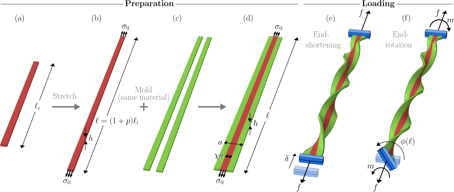
We investigate the model system shown schematically in Fig. 1: an elastic ribbon with a discontinuous distribution of pre-stress in the cross-section, prepared as follows. Starting with an elastic strip with a uniform and rectangular cross-section (Fig. 1a), we apply a uniaxial strain so that its length becomes multiplied by a factor (Fig. 1b); the corresponding stress is . The stretched strip is subsequently bonded along its outer, lateral edges to two identical strips (Fig. 1c). Composed of the same material, the thickness and length of these additional strips exactly match those of the pre-stretched strip when they are unstressed (Fig. 1d). Hence, after bonding, the strips form a ribbon of (constant) thickness , width , and length , in which the pre-stress is non-zero (and tensile) only in an ‘inner’ region of width ; here is the dimensionless area fraction. The inner region lies symmetrically in the cross-section so that the overall distribution of pre-stress is also symmetric. We refer to the configuration in Fig. 1d — in which the outer region (green) is unstressed — as the ‘fully-unrelaxed’ shape. Furthermore, we refer to the system as a ribbon rather than a rod or a plate, owing to its small thickness-to-width and width-to-length ratios: throughout, we consider .
We will explore the mechanical behavior of the ribbon under two loading scenarios.
- 1.
Firstly, starting in the fully-unrelaxed configuration, we allow its ends to shorten by a distance (referred to as the end-shortening) while simultaneously clamping the ends to prevent transverse displacement and rotation; see Fig. 1e. The end-shortening effectively controls the average axial strain in the ribbon, which serves as a control parameter. In general, the ribbon remains planar for small end-shortenings: with symmetric pre-stress, the ribbon cannot relax the pre-stress by developing spontaneous curvature (as occurs with the classical bimetallic strip). Instead, we will show that, above a critical end-shortening, the ribbon undergoes torsional buckling: it deforms significantly out of plane, forming helicoidal-like shapes in which the cross-section twists about the ribbon centerline at a well-defined spatial rate. Broadly speaking, twisting allows the ribbon to relieve some compressive stress in the outer region while the inner region remains under tension.
- 2.
In the second loading scenario (Fig. 1f), we rotate one clamp by an angle about the ribbon axis (which serves as an alternate control parameter) while fixing the end-shortening.
In both loading scenarios, we consider the axial force, , and moment, , exerted on the clamps.
We seek to understand when torsional buckling occurs and how the resulting twisting influences the overall, macroscopic behavior of the ribbon. Specifically, using a 1D ‘rod-like’ model and simulations based on the finite element method (FEM), we characterize the local twist rate (i.e., the rate at which cross-sections rotate about the ribbon centerline) as a function of the applied end-shortening , end-rotation , pre-strain and area fraction . We quantify the macroscopic behavior of the ribbon using the axial force, , and moment, (Figs. 1e–f). We will compare our analytical and numerical results with our experiments on elastomeric samples.
Furthermore, a key feature of the torsional buckling exhibited by our ribbons is that the helicoidal shapes generally exist in regions of alternating chirality (Figs. 1e–f). These regions can be regarded as distinct thermodynamic phases in which the twist rate acts as an order parameter. The phase boundaries between neighboring regions, where the twist rate rapidly changes sign according to the chiralities of the regions, are similar to the perversions observed in elastic rods with intrinsic curvature (Goriely and Tabor 1998; McMillen and Goriely 2002). Following Huang et al. 2012, we also refer to them here as perversions, even though the ribbon has zero intrinsic curvature. The torsional buckling can then be viewed as a phase separation process, in which the planar, homogeneous state becomes unstable to distinct buckled phases that co-exist in equilibrium. In addition to developing a quantitative understanding of the instability, we aim to substantiate this thermodynamic analogy through the analytical insight afforded by the 1D model.
3 Ribbon model of inhomogeneously pre-stressed ribbons
In this section, we develop a theoretical model for an elastic ribbon subject to inhomogeneous pre-stress (as shown in Fig. 1). In particular, we seek a simplified model to gain analytical understanding of the torsional instability. To understand the behavior beyond the onset of buckling, our model needs to account for extensibility of the ribbon mid-surface and finite rotations of its cross-section with respect to the laboratory frame. While a geometrically-exact shell theory may be an obvious candidate, the complexity of the governing equations means that analytical progress is generally not possible. Recently, Audoly and Neukirch 2021 have demonstrated that an extensible ribbon model, accounting for finite rotations, can be systematically derived from a geometrically-nonlinear plate model, using a dimension reduction that is asymptotically valid in the slenderness limit characteristic of ribbons. The result is a 1D ‘rod-like’ model, in which the strain energy is expressed solely in terms of ‘macroscopic’ strains (stretching, bending, twisting) attached to the ribbon centerline.
We adapt the extensible ribbon model of Audoly and Neukirch 2021 to incorporate inhomogeneous, uniaxial pre-stress. Because our derivation up to §3.3 closely follows that proposed by these authors, we do not present all details of the dimension reduction; instead, we outline the main steps of the method and highlight the elements that are different here. Throughout, we will focus on steady deformations, i.e., we suppose that the end-shortening and end-rotation are applied quasi-statically. For simplicity, we assume that both inner and outer regions (Fig. 1d) are composed of the same isotropic, homogeneous material. In addition to the slenderness assumption , we assume a small pre-strain, , as well as small strains during end-shortening and end-rotation; this requires and (see Figs. 1e–f). Hence, a linearly elastic constitutive law is appropriate, with Young’s modulus and Poisson ratio . Furthermore, because we are primarily interested in a twisting instability, for which the centerline remains approximately straight (Figs. 1e–f), we limit attention to the case of combined stretching and twisting: we only seek solutions with straight centerline (zero bending strains). Together, these assumptions allow us to make significant analytical progress. Later, we will compare our predictions with numerical simulations and experiments for which the strains are not necessarily small, demonstrating good quantitative agreement despite the ribbon model being formally valid only for small strains.
3.1 Kinematic description of the ribbon
To facilitate the dimension reduction, we describe the ribbon kinematics using a centerline and a set of orthogonal directors (Fig. 2). Throughout this section, we take our reference state to be the fully-unrelaxed configuration shown in Figs. 1d and 2a, i.e., we define displacements and strains relative to this configuration. We take Cartesian coordinates in the laboratory frame such that the reference mid-surface lies in the plane, with the -axis parallel to the ribbon centerline (Fig. 2a); the ribbon ends correspond to and . The corresponding unit vectors in Cartesian coordinates are . We also define material coordinates along the longitudinal and transverse directions, respectively, where and (thus, in the reference configuration, we can identify and ). The reference configuration has a resultant pre-stress (defined as the bulk stress integrated over thickness) that is uniaxial in the longitudinal direction, denoted . This has the form (Fig. 2a):
| (1) |
where, under the assumption of linear elasticity, .

In the deformed configuration, we denote the centerline of the ribbon (defined to be the centroid of the cross-section for each ) by ; see Fig. 2b. Under the assumption of zero centerline bending, the tangent vector is everywhere parallel to the -axis:
| (2) |
where is the macroscopic axial strain relative to the reference configuration, controlled (indirectly) by the imposed end-shortening.
To complete the description of the local orientation of the ribbon, we introduce the vectors and (referred to as directors in the Kirchhoff theory of rods) such that forms a right-handed orthonormal basis for each . In the absence of centerline bending, and are simply a rotation of the Cartesian unit vectors and , respectively, about the -axis (Fig. 2). Denoting the angle of rotation by , we have
| (3) |
The twisting strain (spatial rate of twist), denoted , is
| (4) |
To characterize how the ribbon deforms within each cross-section, we introduce the displacement components in the director basis, , such that the deformed position of the point with material coordinates is
| (5) |
The ‘macroscopic’ strains and — characterizing the average deformation of each cross-section — together with the ‘microscopic’ displacements complete the kinematic description of the ribbon. It is also necessary to include the following kinematic constraints. Because we define the centerline to be the centroid of each cross-section, we must impose that the displacements have zero mean over the interval :
| (6) |
An additional constraint is needed to remove any indeterminacy in the definition of and ; from Eq. (3), this is equivalent to uniquely specifying the twist angle for each . We require that indeed corresponds to an ‘average’ twist angle of the cross-section about the -axis, in the sense that the first moment of the out-of-plane displacement is zero:
| (7) |
Before proceeding, we determine the orders of magnitude of the macroscopic strains in terms of the ribbon parameters. These scalings inform which terms to retain in a weakly-nonlinear plate model of the ribbon, before any dimension reduction is applied. Following Audoly and Neukirch 2021, we perform a scaling analysis in the limit under consideration, assuming that (i) the stretching and twisting contributions to the elastic energy all balance at leading order; and (ii) the in-plane strain can be estimated from twisting over a lengthscale comparable to the plate width . This yields11 1 The scalings in Eq. (8) are equivalent to those in Audoly and Neukirch 2021, up to coefficients of order 1.
| (8) |
3.2 Elastic energy of homogeneous solutions
We denote the in-plane (membrane) strain components by and the bending strains by ; here and throughout, Greek indices are limited to the in-plane directions, . By first calculating the deformation gradient associated with in Eq. (5), then expanding terms using the scalings in Eq. (8), the dominant contributions to the strains in the limit were calculated by Audoly and Neukirch 2021. These strains are geometrically nonlinear and account for gradients in both the macroscopic strains and microscopic displacements along the ribbon centerline. In our following analysis, we neglect gradient effects along the centerline by limiting attention to ‘homogeneous solutions’, independent of the longitudinal coordinate :
| (9) |
Given the separation of lengthscales inherent to the ribbon geometry, this simplification is asymptotically valid when are no longer independent of but vary on a lengthscale much larger than the ribbon width . More precisely, the minimizers of the resulting elastic energy (subject to appropriate boundary conditions) are the dominant contribution when the solution of the full system is expanded in the limit (Hodges 2006; Audoly and Lestringant 2021). The gradient terms involving -derivatives of only enter the expansion at higher order.
Considering homogeneous solutions of the form (9) with zero centerline bending, the strain components simplify to (primes now denoting derivatives)
| (10) |
In the absence of the macroscopic strains and , the above equations reduce to the usual (weakly-nonlinear) von Kármán strain-displacement relations for plates, as expressed in a Cartesian frame. Note that the longitudinal strain is the macroscopic strain plus a contribution depending on the transverse coordinate , which captures the fact that, in the presence of twisting, fibers initially parallel to the centerline are deformed into helices with helical radius . Thus, twisting induces longitudinal extension that is more pronounced on the edges of the ribbon, where is larger. This explains why helical buckling can effectively relax compressive pre-stress that is localized along the edges of the ribbon.
Owing to the small thickness , the elastic energy and constitutive relations are now calculated in the framework of classical thin-plate theory. The total strain energy associated with homogeneous solutions is , where is the strain energy per unit length. In the presence of uniaxial pre-stress , we can write as (using Einstein notation for summation over repeated indices)
| (11) |
where is the stiffness tensor ( is the Kronecker delta):
The constitutive laws for the resultant membrane stresses, , are then derived from Eq. (11) as
| (12) |
and similarly for the resultant bending stresses, :
| (13) |
These expressions resemble the standard constitutive relations for thin (non pre-stressed) plates, with an additional term arising from the uniaxial pre-stress .
3.3 Dimension reduction via relaxation of microscopic displacements
Substituting the expressions in Eq. (10) for the strain components, the strain energy in Eq. (11) can be written as a functional of the microscopic displacements and macroscopic strains:
For each combination of (constant) strains , the displacements are determined by the condition that is stationary subject to the kinematic constraints in Eqs. (6)–(7). This ‘relaxation’ procedure allows us to eliminate in favor of , leading to a 1D rod-like theory with energy density along the ribbon centerline.
The relaxation procedure is presented in AppendixA. The key result is that, as in the case without pre-stress considered by Audoly and Neukirch 2021, it is possible to reduce the Euler-Lagrange equations for to a fourth-order boundary-value problem for the out-of-plane component, . The solution is unique and is given by for all : with zero centerline bending, cross-sections rotate about the straight centerline and remain straight. Note that they can still stretch or contract by a Poisson effect, as in general. The solution is considerably more involved when centerline bending or strain gradients are considered.
After applying the relaxation procedure, the strain energy in Eq. (11) reduces to (see AppendixA)
| (14) |
Here and are (constant) strains that depend on the distribution of pre-stress in Eq. (1):
| (15) |
where here, and in later equations, and denote averages over the ribbon width and length, respectively:
As discussed in §2, we subject the ribbon to global constraints via the end-shortening and end-rotation . These constraints impose, respectively, an average axial strain and twist strain along the ribbon centerline, . Therefore, we have
| (16) |
3.4 Interpretation of the pre-stress coefficients and
To interpret the quantity , we consider the longitudinal force (tension) in the absence of twisting ():
In the fully-unrelaxed configuration, the longitudinal force is tensile, , as by Eq. (15). We also have , implying that is the (negative, hence contractile) overall strain at which the tension goes from positive to negative when the ribbon is allowed to shorten. For a very long ribbon, , the condition of Euler buckling is precisely that the longitudinal force goes through zero; the buckling threshold is therefore
| (17) |
recalling that . This is consistent with the fact that is defined in Eq. (15) as proportional to the average pre-stress.
Next, we consider the term in square brackets in Eq. (14). Appearing in a factor of , it can be interpreted as an incremental (scaled) twisting modulus, and we anticipate that torsional buckling occurs when this quantity vanishes, i.e., when where
| (18) |
In the right-hand side, the term captures the stabilizing effect of the plate’s bending modulus (the larger , the more negative the critical strain ), the term captures the stabilizing effect of the longitudinal force (overall tension), and the term captures the effect of the pre-stress inhomogeneity on the twisting rigidity, as can be seen from its definition in Eq. (15). The pre-stress is more compressive on the sides of the ribbon (larger ) than near the centerline (smaller ), causing to be negative; hence the term in Eq. (14) points to a destabilizing effect of the pre-stress inhomogeneity on torsional buckling.
3.5 Non-dimensionalization
Before proceeding to solve the 1D model, we non-dimensionalize by setting
| (19) |
where we have introduced the slenderness parameter
| (20) |
We note that, using the scaling behavior , the scales used to non-dimensionalize and are precisely those reported earlier in Eq. (8). We also emphasize the minus sign used to non-dimensionalize the end-shortening , in agreement with the usual convention that a contractile strain is counted negative: both and are negative for compression (when ), and become more negative as the end-shortening increases.
Using the definition of in Eq. (18), and applying the above re-scalings, the strain energy in Eq. (14) becomes
| (21) |
where , , and are the re-scaled axial strain, pre-strain, critical strain for torsional buckling, and twisting strain, respectively, and is the area fraction occupied by the inner (pre-stressed) region. After substituting the expressions in Eq. (15) for and , the critical strain in Eq. (18) becomes, in re-scaled form,
| (22) |
The constraints in Eq. (16) are equivalent to
| (23) |
i.e., the average values of and along the ribbon must match the target values and imposed by the clamps.
3.6 Convexification and constitutive laws of the 1D model
The dimensionless energy landscape as a function of the strain variables and is shown in Fig. 3a. This landscape is symmetric as , as required by Eq. (21). We observe two valleys (solid blue curves) where , which emerge from the point on the surface where (labeled ). Using Eq. (21), these valleys are given by
| (24) |
Hence, as the axial strain quasi-statically decreases from zero (i.e., as the end-shortening increases), equilibrium solutions with non-zero twist are first observed at (where from Eq. (22)). Furthermore, as suggested by Fig. 3a, the planar, untwisted solution, , is a local energy minimum as varies (for fixed ) when (solid blue curve above point ), and a local energy maximum when (dashed blue curve). The point corresponds to a supercritical pitchfork bifurcation, in which the planar solution becomes unstable to the pair of stable, buckled solutions with opposite chiralities, .

Because we control only the average axial strain and twist rate via the end-shortening and end-rotation, we must account for possible co-existence of buckled phases along the ribbon length. This is achieved by a convexification of the energy landscape in Fig. 3a, the result of which is shown in Fig. 3b. The non-convex part of energy surface, bounded by the curves , is replaced by a ruled surface (shaded blue). This ruled surface is swept by the line segments that join points and for each .
Physically, the energy convexification may be interpreted as follows. For specified and , one possible solution is the homogeneous buckled configuration with and everywhere along the ribbon. Now suppose that the point lies inside the non-convex region, as represented by the point in Fig. 3a. After convexification (Fig. 3b), the point is projected onto the point lying on the ruled surface: the homogeneous solution is not the global energy minimum, and the system adopts a lower energy state by forming a mixture of buckled phases while conserving the average twist rate22 2 Here we consider only global energy minima. We ignore metastable homogeneous solutions (with and everywhere along the ribbon), which exist in the region bounded by the coexistence curves and the spinodal curves that emerge from the point (defined as the locus of inflection points where ) (Jones 2002); using Eq. (21), this region is . Because we always start with zero average twist () before quasi-statically increasing/decreasing in simulations and experiments, these metastable states are not observed.. Because generators of the ruled surface are evidently parallel to the -axis, the buckled phases in the mixture (corresponding to the points ) everywhere have
| (25) |
The reduced ribbon energy (21) therefore predicts the existence of buckled phases that possess opposite chiralities, but, without higher-order gradient terms, cannot describe perversions (phase boundaries). However, if the point instead lies outside the non-convex region, this conclusion does not hold: since , it is not possible to satisfy point-wise while conserving the average value (as required by Eq. (23)). Thus, in this latter case, phase separation does not occur and the system instead adopts the homogeneous phase .
Using Eqs. (21) and (25), the convexified strain energy, labeled , can be written in terms of the average strains and as
| (26) | |||||
The corresponding effective constitutive laws for the dimensionless equilibrium force, , and moment, , are
| (27) |
| (28) |
We refer to these constitutive laws as ‘effective’ because, in being derived from the convexified strain energy, they account for a mixture of buckled phases inside the non-convex region.
In Fig. 4, we use these expressions to construct surface plots of the force and moment as a function of and . More precisely, in panel (c) we plot the negative moment, , as this quantity turns out to be the analog of pressure in the classical theory of first-order phase transitions (see §3.7 below). To help interpret each of these plots, in Fig. 4d we show example shapes of the ribbon corresponding to the points – on Fig. 4c; these shapes were generated using the FEM simulations discussed in §4.1. (We only draw the shapes for positive applied twist, ; due to symmetry, the shapes for negative twist are found by simply inverting the chiralities.) These shapes are colored red/blue according to the sign of the local chirality, with green regions corresponding to places where the twist rate is approximately zero.

3.7 Thermodynamic analogy: torsional buckling as a phase separation process
The torsional buckling predicted by the ribbon model has many features in common with other critical phenomena described by the classical theory of thermodynamic phase transitions (Sears and Salinger 1975; Selinger 2016). For example, the mixture of buckled phases observed for is analogous to the phase separation of a real gas into its liquid and vapor phases when the temperature is lowered below the critical point, as described by van der Waals theory (Sears and Salinger 1975). In fact, Fig. 4c may be directly compared to the standard pressure-volume-temperature (or “--”) diagrams for the liquid-gas transition in real substances (ignoring solid phases). Therefore, we have the correspondence:
In particular, the average twist rate (as controlled by end-rotation) changes the relative proportion of the two chiralities, similarly to how the system volume determines the relative proportion of liquid and vapor phases. The level curves along which is constant (black curves in Figs. 4a and 4c) can be viewed as isotherms; the bifurcation point is analogous to the critical point, with the critical temperature.
As the system moves quasi-statically between the points – in Fig. 4c, the ribbon shapes in Fig. 4d also highlight a phenomenon that is well known in the theory of thermodynamic phase transitions: depending on the path taken, it is possible to move between two given points with or without phase separation occurring (for example, compare the paths and ).
4 Methodology: numerical and physical experiments
To test the predictions of the extensible ribbon model developed in the previous section, and explore its limits of validity, we also performed computer simulations and desktop-scale experiments. In this section, we begin with a discussion of the numerical simulations in §4.1 and then move on to discuss experimental methodology in §4.2. We delay a discussion of the corresponding results until §5.
4.1 Finite element simulations of pre-stressed ribbons
We conducted simulations based on the finite element method (FEM) using the commercial package Abaqus (Dassault Systèmes, Simulia Corp.). The ribbon was meshed using 3D solid elements with quadratic interpolation order (isoparametric, hexahedral elements with reduced integration; type C3D20R in Abaqus with default element controls). We found that using regular, cuboidal elements of side length (i.e., four elements through the thickness) was sufficient to obtain a converged mesh. The values of physical parameters were chosen to exactly match their experimental counterparts (provided below in Eq. (30)), and were expressed in the millimeter-tonne-second variant of SI units. The discretization comprised elements in each cross-section and elements along the longitudinal direction (86400 total elements).
Material constitutive behavior
To compare our simulations to experiments on elastomeric ribbons (described in §4.2), we implemented an isotropic, nearly-incompressible neo-Hookean material model (Poisson ratio ). (Volumetric locking was avoided by using reduced-integration elements.) While several compressible formulations of the neo-Hookean model have been proposed (Pence and Gou 2015), we used the default form in Abaqus; this formulation arises as a special case of the more general Mooney-Rivlin solid (Bower 2009) and has been successfully used to simulate the behavior of elastomers (Zhao et al. 2019; Yan et al. 2023). In terms of the principal stretches (), the strain energy density (i.e., energy per unit of reference volume) is
| (29) |
where and are the shear and bulk modulus, respectively, and is the volume ratio.

Numerical protocols
Instead of explicitly simulating the two-stage stretching and bonding process used to prepare the ribbons (Figs. 1a–d and experimental fabrication in §4.2), we directly constructed the fully-unrelaxed configuration in our simulations; see Fig. 5a. This step was achieved by first defining the inner and outer regions of the ribbon separately, before merging them so that the mesh naturally retained the internal boundary between the regions. In this way, the pre-stress could be imposed in the inner region as a pre-defined field (via the *FIELD option in Abaqus). For a specified pre-strain , the corresponding uniaxial pre-stress, , was derived from the neo-Hookean energy density (29); for details see AppendixB.
Once the fully-unrelaxed configuration was defined, we conducted FEM analyses under end-shortening and end-rotation. In both loading scenarios, one extremity of the ribbon was clamped by imposing zero displacements at all nodes on the face. At the other extremity, the end-shortening and end-rotation were imposed via a kinematic coupling (Abaqus option *COUPLING) between nodes on the face and a reference point. Throughout, we considered quasi-static loading conditions, using the Abaqus/Standard solver (activating the NLgeom option to incorporate geometric nonlinearities). In addition to the shapes presented earlier in Fig. 4d, Fig. 5b shows an example buckled shape with the numerical mesh superimposed; here we specified the parameter values in Eq. (30) with , , and .
To avoid convergence issues at the buckling onset, we seeded the buckling instability using shape imperfections. To obtain the shape imperfections for each pre-strain , we performed a preliminary eigenvalue buckling analysis under incremental changes to the end-shortening, using the planar, unbuckled solution as the base state. The corresponding node displacements for the first ten eigenmodes were then superimposed onto the fully-unrelaxed configuration (*IMPERFECTION option in Abaqus); the modes were scaled to have amplitudes that geometrically decreased with mode number, with the largest amplitude (first buckling mode) having a maximum displacement component equal to of the ribbon thickness. Furthermore, to obtain reliable results that are insensitive to small changes in mesh size and other numerical parameters, it was necessary to include numerical stabilization to deal with the rapid variation in displacements upon buckling (we used adaptive automatic stabilization in Abaqus with default parameter values). By smoothly ramping the rate at which the end-shortening or end-rotation was applied (from zero to the constant value used throughout each loading step), we ensured that the ratio of viscous dissipation energy to the total strain energy always remained less than ; thus the loading was approximately quasi-static.
Post-processing of numerical data
We extracted the raw simulation data output from Abaqus for post-processing in MATLAB, using the toolbox Abaqus2Matlab (Papazafeiropoulos et al. 2017). The components of the force and moment resultants were readily obtained from the force and moment exerted on the reference point that was coupled kinematically to one extremity of the ribbon. To obtain the twist rate for each material coordinate , we first calculated the local director frame using the raw data of node positions along the ribbon mid-surface; this procedure is detailed in AppendixC. Figure 5c shows a typical twist profile determined with this approach (plotted as a function of deformed arclength for comparison), corresponding to the buckled shape shown in Fig. 5b. By determining the director frame, we can also (i) compute the bending strains and, hence, verify that torsional buckling generally occurs with negligible centerline bending, as was assumed in the ribbon model; and (ii) analyze the behavior in regimes where a bending instability occurs (discussed in §5). Once the local twist rate was determined, we computed its root mean square (RMS), ; as in §3, denotes the average over the ribbon length, .
4.2 Experimental methods
We performed precision desktop-scale experiments on ribbons composed of vinyl polysiloxane (VPS, Elite Double 32, Zhermack) — a silicone-based elastomer whose behavior has been shown to be well approximated, up to strains of around , by a neo-Hookean constitutive law with Young’s modulus and Poisson ratio (Baek et al. 2021; Johanns et al. 2021; Grandgeorge et al. 2021; Grandgeorge et al. 2022). We first describe the procedure used to fabricate the ribbons, before discussing the apparatus and methods we employed in the loading tests.

Fabrication of elastomeric ribbons
To fabricate VPS ribbons with inhomogeneous, uniaxial pre-stress and specified geometric parameters (given below in Eq. (30)), we implemented the two-stage fabrication process summarized earlier in Figs. 1a–d. We custom-made molds from acrylic plates (thickness ; TroGlass Clear Cast, Trotec) that were cut to shape using a laser cutter (Trotec Speedy 400) and bonded together (Acrifix, PLEXIGLAS). For each fabrication stage, a mixture of VPS base and catalyst, in a 1:1 ratio by weight, was placed in a centrifugal mixer (THINKY ARE-250) for a total of seconds ( at rpm clockwise, at 2200 rpm counterclockwise). To minimize imperfections due to air bubbles, the mixture was degassed in a vacuum chamber before being injected into the mold using a syringe (Sano et al. 2022). Curing of the polymer mixture took place at room temperature.
The mold for the first fabrication stage featured a uniform rectangular channel with additional end pieces, to cast the inner strip with ‘clamping blocks’ at its ends. The geometry of this channel had to be tailored to each pre-strain to ensure that the inner strip had the specified thickness , width , and length after uniaxial stretching (specifically, the channel thickness , width and length with Poisson ratio , which compensated for the transverse contraction due to Poisson effects). We added a small amount (less than by weight) of red silicone pigment (Silc Pig, Smooth-On) to the VPS mixture before curing the inner strip so that the pre-stressed region could be visualized in the finished ribbon. For the second fabrication stage, a second mold held the inner strip under the specified uniaxial strain, using the clamping blocks to place it symmetrically in the center of a wider channel (width ) while the outer strips cured around it. This ensured, in turn, that the distribution of pre-stress in the finished ribbons was sufficiently symmetric that they did not develop spontaneous curvature after the mold and clamping blocks were removed. We note that cross-linking of the VPS polymer, at the interface between the inner and outer strips, effectively bonded the strips during the second curing stage without the need for gluing. Each finished sample was left for at least hours before being used for loading tests.
Apparatus and protocols used for loading tests
Analogously to the FEM simulations, we conducted the two types of mechanical tests (end-shortening and end-rotation; see Figs. 1e–f) on our experimental samples. A photograph of the apparatus is shown in Fig. 6. Each ribbon was initially clamped in its fully-unrelaxed configuration to a universal testing machine (Instron 5943). The sample was clamped with the ribbon’s width parallel to the direction of gravity, to minimize sagging due to self-weight. During loading, a torsional load cell (Instron; force capacity , torque capacity ) simultaneously measured the axial force and torque. We also recorded the shape of the ribbon using a digital camera (Nikon D850).
4.3 Parameter values used in the present study
The values of geometric parameters (defined in §2) used throughout this paper are
| (30) |
For each combination of pre-strain and area fraction , we varied the end-shortening in the range (for ) and (for ); larger end-shortenings were required to buckle the ribbon for larger . In both simulations and experiments, we used a loading rate of (for ) and (for ). For the end-rotation tests, we varied the rotation angle in the range (simulations) and (experiments) at a constant angular velocity . In both loading tests, there were no noticeable oscillations of the ribbon, and we verified that changing the rate of loading did not change the results, indicating that the conditions can be regarded as quasi-static. The choice of the above loading rates represents a balance between ensuring quasi-static conditions (in particular, minimizing the viscous dissipation used in the numerical stabilization), while avoiding excessive simulation or experimental times.
5 Results of inhomogeneously pre-stressed ribbons under end loads
In this section, we show that our FEM simulations are able to reproduce the main qualitative features of the torsional buckling exhibited by experimental samples, despite differences in the detailed post-buckled shape. We will also demonstrate that a quantitative agreement can be obtained between the results of FEM simulations and experiments when we consider global quantities that are insensitive to the microscopic buckling pattern. By their nature, these quantities do not rely on finite-length (gradient) effects and so can also be predicted by the ribbon model developed in §3, thus enabling a direct comparison between all three types of analysis. We begin by presenting the results for loading by end-shortening in §5.1, and then for end-rotation in §5.2.
5.1 Torsional buckling under end-shortening
In a first test to validate the FEM simulations against experiments, in Figs. 7a–b we compare the sequence of ribbon shapes obtained under end-shortening for a pre-strain and area fraction . We find excellent qualitative agreement between some features of the simulations and experiments, especially regarding the onset of torsional buckling and subsequent separation into distinct buckled phases. However, we also note differences in the precise buckling pattern that is obtained, including the location and number of perversions: two perversions arise in the experiments as opposed to four in the simulations. We attribute these differences in the buckling pattern to experimental imperfections, as discussed further in §6.

To quantitatively examine the buckling behavior, we consider the twist rate, , along the ribbon centerline. In Fig. 7c, we present a density plot of as a function of end-shortening and material coordinate (undeformed arclength) for the same simulation used to generate the shapes in Fig. 7b. This plot was obtained using the post-processing procedure described in §4.1 so that each vertical slice through the plot (i.e., a line of constant ) corresponds to a twist profile akin to that of Fig. 5c (though now plotted as a function of ). Compared with the numerical shapes (Fig. 7b), the onset of torsional buckling at and phase separation is now more clearly visible. As expected, the magnitude of the twist rate associated with each phase grows as the end-shortening increases. For end-shortenings well beyond the onset of buckling, the twist rate is approximately constant throughout each buckled phase, only varying significantly in the narrow perversions that separate neighboring phases and at the clamped extremities of the ribbon.
While the density plot, , in Fig. 7c helps visualize the twist distribution along the ribbon, it cannot be directly compared to the ribbon model. To enable such a comparison, we consider the root mean square (RMS) of the twist rate, . Because perversions are confined to regions whose length is comparable to the ribbon width (), the RMS twist rate should provide a good approximation to the magnitude of the preferred twist in the buckled phases (this magnitude is equal in both phases due to the symmetry of the system as ). This is shown in Fig. 7d (solid curve) using the simulation data from Fig. 7c. We observe excellent agreement with the equilibrium twist predicted by the ribbon model (dashed curve): recalling the non-dimensionalization in Eq. (19), the dimensional prediction is , where is defined in Eq. (24). The sudden growth in the twist rate at buckling closely follows the behavior expected from Eq. (24), namely near the critical end-shortening . While the numerical curve varies smoothly from the planar, untwisted configuration due to the presence of shape imperfections in our FEM implementation (discussed in §4.1), it is helpful to define an empirical buckling onset for FEM simulations — hereon, we consider the first value of the end-shortening at which the dimensionless RMS twist rate, , exceeds , yielding the points represented by the star symbols in Figs. 7d–e.
Furthermore, the buckling behavior can be quantified by the axial force in the ribbon. In Fig. 7e, we plot the axial force for the same simulation used for Figs. 7b–d (solid curve). We have also superimposed experimental results (circles) and the model prediction (dashed curve), where was given by Eq. (27) (setting in the absence of end-rotation). We obtain good agreement between all three sets of data. The change in slope upon torsional buckling, as predicted from the ribbon model (Eq. (27) and Fig. 4b), is clearly evident in the numerical and experimental curves.
Other values of the pre-strain
In Figs. 8a–d, we show the RMS twist rate and dimensionless axial force, , during end-shortening for a range of pre-strains and area fractions . These plots are presented in dimensionless form, using the non-dimensionalization (19) introduced in §3.

Results for a smaller area fraction () are shown in Figs. 8a–b.
- 1.
In terms of the RMS twist rate (Fig. 8a), we generally obtain excellent agreement between the results from FEM simulations (solid curves) and the ribbon model (dashed curves), despite the model being formally valid only for small strains, . For clarity, however, here (and in Fig. 8c) we have reduced the line thickness of each numerical curve once the axial force becomes negative, indicating that the ribbon is under net compression: soon after this point, the ribbon centerline bends to form an arch shape, similar to classical Euler buckling of a compressed column. The numerical curve then abruptly deviates from the theoretical prediction since the model assumes zero centerline bending.
- 2.
The force-displacement curves from FEM simulations (Fig. 8b) generally agree well with the theoretical prediction in Eq. (27), though we observe a systematic discrepancy for larger pre-strain . Because this discrepancy becomes more significant as increases, it is likely due to the nonlinear elastic response in the neo-Hookean material model (29) used in FEM simulations (the ribbon model assumes a linear constitutive relation). For each pre-strain , the numerical curve displays a clear change in slope at the onset of torsional buckling (stars), which matches up well with the theoretical prediction (given by the red dashed-dotted curve as varies). A typical shape of the ribbon after torsional buckling (corresponding to the point labeled (e)) is shown in Fig. 8e. However, for the smallest pre-strain, , the numerical curve crosses (black dotted line) before any significant change in slope is observed; the ribbon shape in this case confirms that a bending instability occurs before torsional buckling (see Fig. 8f).
- 3.
In addition, Fig. 8b displays experimental data for the pre-strains and (circles). These generally agree well with the analytical and numerical results except when the axial force becomes very small, when we observed significant sagging of the ribbon due to gravitational forces in experiments.
Results for a larger area fraction () are shown in Figs. 8c–d.
- 1.
When the pre-strain , we again observe good agreement between theory and FEM simulations in terms of the RMS twist rate (Fig. 8c) and axial force (Fig. 8d). In particular, the empirically-determined onset of torsional buckling (stars) is well approximated by (defined in Eq. (22)) for each of these pre-strains (red dashed-dotted curve in Fig. 8d). Similar to the case, as the end-shortening is increased further, the numerical curves suddenly deviate from the theory soon after the point where the axial force crosses zero (indicated by a reduced line thickness) and a bending instability occurs (Euler buckling).
- 2.
However, a different picture is obtained for larger pre-strains : along these numerical curves, torsional buckling sets in much earlier than what is predicted by the ribbon model (Fig. 8d), leading to significant discrepancies throughout the entire range of end-shortening. By comparing a typical ribbon shape in this regime (Fig. 8g with the corresponding shape for (Fig. 8e), we find that the buckling mode is qualitatively different, being microscopic in nature for : the wavelength is comparable to the ribbon width, , leading to a large number of perversions (typically or more). Furthermore, for even larger (not shown here), the buckling shifts to being microscopic and of bending type, resembling a wrinkling instability. As discussed in §6, both types of microscopic buckling lie outside the validity limit of the ribbon model.
In summary, we have a competition between macroscopic helical buckling and Euler buckling for a smaller area fraction (), and a competition between these two modes plus microscopic buckling for larger area fraction ().
5.2 Behavior of pre- and post-buckled ribbons under end-rotation
Next, we consider how the relative proportion of the buckled phases depends on the average applied twist. As in the case of end-shortening, we make a first comparison between experiments and FEM simulations during end-rotation by analyzing the sequence of ribbon shapes; see Figs. 9a–b. As in Fig. 7, here we have taken and , though now we fix the end-shortening at . We obtain a similar picture: the simulations capture the key qualitative features of the experimental system despite differences in the detailed buckling pattern. As the end-rotation increases, we observe the propagation and annihilation of perversions in both the experiment and simulation, with the system eventually reaching a homogeneous state characterized by a single chirality.

For the numerical simulation shown in Fig. 9b, the density plot of the twist rate (with end-rotation now being the second variable, in addition to the material coordinate ) is shown in Fig. 9c. This plot shows how the four perversions that are initially present propagate and abruptly disappear as they collide with the clamped boundaries and each other. Note that remote parts of the ribbon, including other perversions, undergo sudden re-arrangements after such events. After the system reaches a single, global chirality for large rotations, the associated twist rate becomes uniform along the ribbon (except near the extremities due to boundary effects).
In Fig. 9d, we plot the corresponding FEM-computed axial moment, (solid curve), as a function of end-rotation, together with experimental results (circles) and the prediction from the ribbon model (dashed curve), where is evaluated using Eq. (28). Here, we obtain larger quantitative differences compared to the analogous load-displacement curve during end-shortening (Fig. 7e). Nevertheless, the three data sets exhibit the same qualitative features, including the plateau where for small rotations and subsequent stiffening for .
Other values of the pre-strains
The negative axial moment during end-rotation for several end-shortenings is shown in Fig. 10 (plotting dimensionless quantities as defined in Eq. (19)), for an area fraction and pre-strain (Fig. 10a) and (Fig. 10b). These plots are similar to the theoretical surface presented in Fig. 4c. In particular, the predicted plateau in the convexified region (highlighted blue) is evident in the numerical and experimental results. For each end-shortening, the value of at which the moment starts to increase rapidly generally matches up well with the coexistence curves (blue curves). However, for values , the ribbon model systematically underestimates the numerical data when large twisting strains are encountered; similar to the discrepancy observed in the axial force for larger pre-strains in Figs. 8b and 8d, we expect that the discrepancy observed at large twist is due to nonlinear terms in the neo-Hookean constitutive law that are neglected by the ribbon model.

6 Limitations of our ribbon model
In comparing the quantitative predictions of the ribbon model with FEM simulations and experiments in §5, we generally found good agreement with macroscopic quantities that are insensitive to the precise buckling pattern — such as the RMS twist rate and axial force — except in two regimes. First, a macroscopic instability occurs when the axial force transitions from tensile to compressive, which is characterized by significant centerline bending (Euler buckling). This bending instability is generally encountered as the end-shortening is increased beyond the onset of torsional buckling, but, for sufficiently small pre-strain , centerline bending occurs before torsional buckling (Fig. 8f); in the latter case, no twisting instability is observed, even as the end-shortening is increased further. In the second regime, generally encountered for larger and large pre-strain , the initial instability is microscopic (see Fig. 8g): the buckling wavelength instead of , being associated with a large number of perversions (or wrinkles for even larger , when the microscopic instability shifts to being of bending type) that persist upon further end-shortening.
The two regimes mentioned above cannot be described by our ribbon model due to two assumptions made in §3: (i) centerline bending is negligible, and (ii) variations in the strains occur on lengthscales much larger than the ribbon width. While it would be possible to incorporate centerline bending into the ribbon model (recall the discussion at the start of §3), the assumption (ii) lies at the heart of the dimension reduction and cannot be relaxed. Indeed, as well being unable to predict microscopic instabilities, the ribbon model cannot describe deformations in the vicinity of perversions nor finite-length effects such as the number/location of perversions. In future work, we will try to account for the microscopic instabilities by returning to the plate model used as a starting point for the dimension reduction.
6.1 Competition between torsional and Euler buckling
Equations (17) and (18) yield the critical strain for Euler versus torsional buckling, respectively. These two values are mutually exclusive as they both characterize the stability of the same flat configuration: we should limit attention to whichever instability occurs first during end-shorting. Specifically, torsional buckling occurs before Euler buckling when (recall that both quantities are negative), which corresponds to
| (31) |
Physically, this states that the destabilizing effect of non-uniform pre-stress (as encapsulated in ) outweighs the stabilizing effect of bending stiffness.
For the particular distribution of pre-stress considered in this paper, i.e., Eq. (1), we have and the above condition can be re-arranged to
| (32) |
In dimensionless terms, it follows from Eq. (27) that this is precisely the statement , i.e., the axial force is positive (tensile) at the onset of torsional buckling when ; here the critical value is as defined in Eq. (22).
6.2 Phase diagram of buckling
Combining the above discussion with our numerical results from §5, we can construct a phase diagram of the initial instability that occurs as the end-shortening is quasi-statically increased (starting in the fully-unrelaxed configuration); this is shown on the -plane in Fig. 11a, where is the area fraction occupied by the pre-stressed region and is the re-scaled pre-strain (with as defined in Eq. (20)). Here, we have plotted points corresponding to the values of and used in the FEM simulations (reported in Eq. (30)), with symbols corresponding to the type of instability observed in §5.1: these are macroscopic bending (Euler-type) in region I (squares), macroscopic twisting-type in region II (circles), and microscopic twisting/bending-type in region III (triangles). In addition, we have included the boundary of regions I and II predicted by the 1D model (black curve), given by , using the expression for in Eq. (32). The square symbols at the bottom of the each stack of symbols, corresponding to , both fall below this boundary, in region I. This is consistent with our observation in §5.1 of an Euler instability for this value of .

To help interpret the diagram, in Fig. 11b we show typical force-displacement curves, obtained from FEM, for each of the regions I–III (these are reproduced from Fig. 8d for and various pre-strains , , ). Figure 11c also displays representative buckling modes. Euler buckling (I) occurs when the force-displacement curve (dark blue curve in the lower left corner of Fig. 8d) reaches (black dotted line) before it intersects the critical strain for torsional buckling (red dashed-dotted curve). The ribbon model can predict the onset of Euler buckling, Eq. (17), though a description of the post-buckled shape would require centerline bending to be incorporated into the model. In region II, macroscopic torsional buckling takes place at the critical strain predicted by the ribbon model (intersection of the light blue and red dashed-dotted curves); the model is also valid in the post-buckled regime, provided a secondary bending instability does not occur. As discussed in §6 above, the onset of microscopic buckling (III) (nor the post-buckled behavior) cannot be predicted by the 1D model (green star symbol lying above the red dashed-dotted curve).
In addition, for illustrative purposes, we have plotted a speculative boundary between regions II and III on Fig. 11a, as well as a guess of the locus of critical points at which microscopic buckling occurs on Fig. 11b (gray dashed curves). Together, these form the limit of validity of the ribbon model. We emphasize that these boundaries are freehand guesses. We expect that their precise form may be determined by a linear stability analysis of the Föppl-von-Kármán plate model, which will be considered in a future publication.
7 Discussion and conclusions
7.1 Summary of findings
In this paper, we have studied elastic ribbons subject to uniaxial pre-stress that is inhomogeneous in the cross-section. In our experiments (discussed in §4.2), we fabricated these ribbons using a stretch-and-bond procedure (cf. Figs. 1a–d) to yield a pre-stress that is non-zero only in a central region of relative area . More broadly, a similar distribution of pre-stress could equally arise in an initially unstressed ribbon, in which the inner region contracts relative to the outer region due to active changes such as growth or inflation (Koehl et al. 2008; Siéfert et al. 2019; Gao et al. 2020; Siéfert et al. 2020; Moulton et al. 2020).
Because the pre-stress is mirror-symmetric about the ribbon centerline, classical 1D models predict zero spontaneous curvature and twist and so are unable to describe the torsional instability. Therefore, the ribbon serves as a model system to test and apply novel dimension-reduction tools when standard theories do not apply. In §3 we adapted the extensible ribbon model recently developed by Audoly and Neukirch 2021 to incorporate pre-stress. This model successfully captures the salient features of the system observed in experiments and numerical simulations: these include when buckled phases co-exist under a controlled end-to-end displacement and rotation, and the preferred values of the twist rate (away from boundaries and perversions). As well as neglecting strain gradients (and hence microscopic instabilities) and describing only solutions with zero centerline bending, a key assumption of the ribbon model is that the strains are small; in particular, the pre-strain satisfies . While the assumption may appear to be overly restrictive, we obtained good quantitative agreement with experiments and FEM simulations for pre-strains up to . In addition, the non-dimensionalization introduced in Eq. (19) indicates that the system depends on only via the re-scaled pre-strain , where is the slenderness parameter defined in Eq. (20). It is for this reason that the phase diagram in Fig. 11a is plotted with on the vertical axis, and the minimum pre-strain for torsional buckling to occur before Euler buckling, , scales as (recall Eq. (32)). It follows that the torsional instability can be observed with arbitrarily small pre-strain by using a strip with sufficiently small thickness-to-width ratio, .
Our ribbon system provides a desktop-scale elastic analog to classical thermodynamic phase separation (e.g., of a real gas into its liquid and vapor phases). Specifically, the mixture of buckled phases occurring for sufficiently negative axial strain (as applied via end-shortening) is analogous to lowering the temperature below the critical point. The average twist rate (applied via end-rotation) changes the relative proportion of the two phases, similarly to how the system volume determines the relative proportion of liquid and vapor phases; the negative axial moment, , which is the conjugate thermodynamic variable to the twist rate, is then analogous to the pressure. Thus, the moment-twist-strain plots, as predicted by the ribbon model (Fig. 4c) and obtained from numerical and experimental data (Fig. 10), are analogous to standard pressure-volume-temperature (“--”) diagrams (Sears and Salinger 1975). We also note that the convexification of the strain energy (Fig. 3b) is similar to the Maxwell construction (also referred to as the equal-area rule) (Clerk-Maxwell 1875). Similar constructions have been used in other problems in elasticity involving co-existing phases in a spatially-extended system, such as bulges in a hyperelastic cylindrical membrane (Chater and Hutchinson 1984); see also Siéfert and Roman 2020 and references therein.
We found that our FEM simulations are able to reproduce the main qualitative features of the experimental system (recall Figs. 7a–b and 9a–b), despite differences in the precise buckling pattern. We attribute these differences to the presence of imperfections in the experiments, both in the ribbon samples and in the clamping conditions. Generally, we expect that the system becomes highly sensitive to imperfections near the onset of buckling. Because the incipient buckling mode is known to control the location of perversions in the related bi-strip studied by Huang et al. 2012 and Lestringant and Audoly 2017, this sensitivity should persist throughout the entire loading history. The sensitivity is also exacerbated by the fact that perversions can move and interact with little energetic cost, as is easily observable experimentally by twisting or poking the ribbon by hand in the vicinity of perversions. As discussed in §3, perversions are associated with higher-order gradient terms in the strain energy, which are asymptotically small compared to the energy associated with longitudinal stretching in the slender limit .
7.2 Discussion and outlook
The phase diagram presented in Fig. 11a provides insight into torsional instabilities observed in other elastic ribbons. While Fig. 11a is only valid for the precise distribution of pre-stress considered here, i.e. Eq. (1), we expect that a similar diagram is obtained whenever the pre-stress (with respect to a suitable reference configuration) is symmetric and more compressive towards the edges than around the centerline. For example, Siéfert et al. 2020, and Gao et al. 2020 were able to program such a stress profile in a patterned fabric strip, which spontaneously adopted a helicoidal shape upon inflation. Similarly, in kelp blades, the growth rate is known to increase with distance from the blade center, and different buckling morphologies of kelp blades have been studied by Koehl et al. 2008. Narrow blades tend to buckle globally to helicoidal shapes, while wide blades buckle microscopically to form ruffled edges. This can be interpreted as moving between regions II and III on Fig. 11a, noting that, for a fixed pre-strain , increasing the width decreases and hence increases the re-scaled pre-strain .
Our system can be useful in understanding torsional instabilities driven by residual stress in other prismatic solids. An example is the ‘twisters’ studied by Turcaud et al. 2011; Turcaud et al. 2020, which are rods composed of two elastic phases with contrasting expansion coefficients (when heated, for example). In numerical simulations, the rods were observed to spontaneously twist by an amount that depends sensitively on the cross-section geometry; in particular, Turcaud et al. 2011 could only obtain significant twisting by connecting flattened ‘wings’ of the high-expansion phase to a compact inner region composed of the low-expansion phase. Noting that the high and low-expansion phases are, respectively, analogous to the outer (initially unstressed) and inner (pre-stretched) regions in our ribbon system, this observation is consistent with the result of Eq. (31): twisting is only observed if the destabilizing effect of non-uniform pre-stress is sufficient to overcome the energy penalty of bending. Due to the flattened cross-section of the ribbon, the outer region naturally resembles the winged geometry of Turcaud et al. 2011.
Finally, our ribbon model can also be useful in developing a quantitative understanding of other torsional instabilities. The 1D energy density that we derived in Eq. (14) can, in principle, be generalized to other cross-section geometries. Provided that there is sufficient symmetry so that the straight, untwisted configuration is always an equilibrium solution, our analysis suggests that only uniaxial twisting and stretching about a straight centerline need to be considered. From this simple kinematic restriction, a similar energy may then readily be derived, which, in turn, should lead to a condition for instability in terms of the geometric parameters for a general cross-section shape. This approach opens up several directions for further study: for example, it can be used as the basis to design rods that become unstable at a pre-programmed threshold. When combined with other types of actuation such as inflation (Siéfert et al. 2019; Siéfert et al. 2020; Jones et al. 2021; Becker et al. 2022), it can potentially be used to develop soft actuators whose deformation in three dimensions can be repeatedly re-programmed during deformation.
Appendix AppendixA Relaxation of microscopic displacements in the ribbon model
In this Appendix, we detail the relaxation procedure used to eliminate the dependence of the strain energy on the microscopic displacements , and hence obtain the reduced energy density reported in Eq. (14). Our analysis follows Appendix A.2 in Audoly and Neukirch 2021, which we modify by (i) incorporating a uniaxial pre-stress and (ii) neglecting centerline bending. We note that the calculation below holds for any distribution of pre-stress, .
Starting with the strain energy (per unit length) defined in Eq. (11), we impose the kinematic constraints in Eqs. (6)–(7) by introducing the four scalar Lagrange multipliers and forming the augmented energy:
Inserting the expression in Eq. (11) for gives
where we define
| (33) | |||||
Substituting the expressions in Eq. (10) for the membrane and bending strains, can be written as an explicit function of , , , and ; however, it is convenient to keep the strains unevaluated for now.
We then perturb the displacements and compute the first variation . Because the membrane and bending strains depend only on the first derivatives of and , the first variation is
where
| (34) |
Integrating by parts over the width to remove all derivatives on the perturbed quantities , the first variation of the functional is
| (35) | |||||
Requiring that the first variation is zero for all admissible , we obtain the Euler-Lagrange equations:
| (36) |
and the natural boundary conditions
| (37) |
Using the expressions in Eq. (34), these simplify to
These correspond to zero transverse membrane stress, shear stress, transverse bending stress and shear force at the ribbon boundaries.
It is possible to reduce Eqs. (36)–(37) to a boundary-value problem for the out-of-plane displacement, . To this end, we integrate the first two Euler-Lagrange equations across the width, and make use of the first two natural boundary conditions in Eq. (37) to yield
Returning to Eq. (36), we see that and are constant. Again using the boundary conditions in Eq. (37), we obtain
i.e., the transverse membrane stress and shear stress are everywhere zero. The remaining partial derivatives in Eq. (34) simplify to
Substituting for and using Eq. (10), the final Euler-Lagrange equation in Eq. (36) becomes
| (38) |
to be solved with the remaining natural boundary conditions in Eq. (37) and the kinematic conditions for in Eqs. (6)–(7):
| (39) |
Furthermore, we can eliminate the Lagrange multipliers and as follows. Integrating Eq. (38) over the width and using gives
Similarly, if we multiply Eq. (38) by before integrating (using parts to integrate the final term), the boundary conditions give
Returning to Eqs. (38)–(39), the boundary-value problem for reduces to
The unique solution is simply ; the equations can then be integrated with the other kinematic conditions in Eqs. (6)–(7) to determine the in-plane displacements as and .
In summary, we have shown that, as a result of relaxation of the microscopic displacements with respect to the macroscopic strains , we have
The strains in Eq. (10) associated with homogeneous solutions then reduce to
| (40) |
The only non-zero components that remain are (i) the longitudinal strain resulting from the macroscopic strain and the stretching that arises due to twist; (ii) the transverse in-plane strain that arises due to Poisson effects; and (iii) the shear strain associated with twisting.
Appendix AppendixB Determining the pre-stress using the neo-Hookean material model
To implement the pre-stress in the framework of the neo-Hookean material model, we identify the principal direction with the longitudinal direction along the fully-unrelaxed ribbon, and the , directions with the transverse directions. Under the applied pre-strain , the principal stretches in the inner region are then
| (41) |
where the volume ratio is to be determined. The Cauchy (true) stresses are derived from the strain energy in Eq. (29) as
| (42) |
After substituting the principal stretches (41), we obtain
| (43) |
Because the pre-stretched strip is initially unconstrained transversely (Fig. 1b), we have , yielding:
| (44) |
Once this equation is solved (using a standard root-finding algorithm) for , the pre-stress can be evaluated using Eq. (43).
We note that in the small-strain limit , ignoring terms of , we have and (making use of the expressions and ), thus recovering the expression for used in the ribbon model (Eq. (1)).
Appendix AppendixC Determining the bending and twisting strains along the ribbon centerline
Here, we describe our method to determine the bending and twisting strains along the ribbon centerline, for each loading step in our numerical (FEM) simulations. Our approach computes the twist angle by averaging data from all mid-surface nodes in a given cross-section, accounting for possible bending of the centerline (associated with rotation of the unit tangent vector). It is therefore robust to warping of the cross-section and distortion of mesh elements. We found that characterizing the twist using a single off-centerline node often gave noisy and inaccurate results.
Starting from the raw data of node positions along the ribbon mid-surface, we first determined the orthonormal director basis ; here is the unit tangent vector (we assumed in the ribbon model derived in §3), and and span the cross-section perpendicular to . Firstly, we obtained the coordinates of all nodes on the centerline, sorted in order of increasing material coordinate (the existence of node points exactly on the material centerline was guaranteed from the symmetry of the mesh). Using centered finite differences on the interior centerline nodes, we then calculated the unit tangent vector, (for the edge nodes, the tangent was unchanged from due to the clamped boundary conditions). Next, we calculated the directors and at each using the coordinate data of all mid-surface nodes in that cross-section. Specifically, we first computed the displacement vectors from the deformed centerline to all mid-surface nodes (components with respect to the global Cartesian frame), which were projected into the plane normal to . This enabled us to calculate ‘trial’ directors and , for example by aligning with the displacement vector to the nearest off-centerline node, and setting . We then computed the plane-polar coordinates of the projected nodes in the trial frame, and defined the average twist angle of the cross-section to be the second (polar) moment of the angular coordinates. This definition is the discrete analog of the kinematic condition (recall Eq. (7)) used to uniquely define the twist angle in the ribbon model. Finally, the directors and were found by rotating the trial directors such that aligned with the average twist angle.
In general, under the requirement of orthonormality, the evolution of the directors along the centerline (parameterized by the material coordinate ) is described by the Darboux vector where
| (45) |
Writing in terms of components in the director basis, i.e., , we can interpret , as the bending strains and as the twisting strain (the rate of twist along ). Thus, with the directors determined on the numerical mesh, the bending and twisting strains were calculated using the following equations, which immediately follow from Eq. (45):
In these expressions, the derivatives were evaluated using centered finite differences on the numerical mesh.
References
- Agostiniani et al. (2017) Agostiniani, V., DeSimone, A., Koumatos, K., 2017. Shape programming for narrow ribbons of nematic elastomers. J. Elast. 127, 1–24.
- Aharoni et al. (2012) Aharoni, H., Abraham, Y., Elbaum, R., Sharon, E., Kupferman, R., 2012. Emergence of spontaneous twist and curvature in non-Euclidean rods: application to Erodium plant cells. Phys. Rev. Lett. 108, 238106.
- Audoly and Hutchinson (2016) Audoly, B., Hutchinson, J.W., 2016. Analysis of necking based on a one-dimensional model. J. Mech. Phys. Solids 97, 68–91.
- Audoly and Lestringant (2021) Audoly, B., Lestringant, C., 2021. Asymptotic derivation of high-order rod models from non-linear 3D elasticity. J. Mech. Phys. Solids 148, 104264.
- Audoly and Neukirch (2021) Audoly, B., Neukirch, S., 2021. A one-dimensional model for elastic ribbons: A little stretching makes a big difference. J. Mech. Phys. Solids 153, 104457.
- Baek et al. (2021) Baek, C., Johanns, P., Sano, T.G., Grandgeorge, P., Reis, P.M., 2021. Finite element modeling of tight elastic knots. J. Appl. Mech. 88, 024501.
- Becker et al. (2022) Becker, K., Teeple, C., Charles, N., Jung, Y., Baum, D., Weaver, J.C., Mahadevan, L., Wood, R., 2022. Active entanglement enables stochastic, topological grasping. Proc. Natl. Acad. Sci. U.S.A. 119, e2209819119.
- Bower (2009) Bower, A.F., 2009. Applied mechanics of solids. CRC press, Boca Raton, FL.
- Brunetti et al. (2020) Brunetti, M., Favata, A., Vidoli, S., 2020. Enhanced models for the nonlinear bending of planar rods: localization phenomena and multistability. Proc. R. Soc. A 476, 20200455.
- Calladine (1975) Calladine, C.R., 1975. Construction of bacterial flagella. Nature 255, 121–124.
- Chater and Hutchinson (1984) Chater, E., Hutchinson, J.W., 1984. On the propagation of bulges and buckles. J. Appl. Mech. 51, 269–277.
- Chen et al. (2016) Chen, Z., Huang, G., Trase, I., Han, X., Mei, Y., 2016. Mechanical self-assembly of a strain-engineered flexible layer: wrinkling, rolling, and twisting. Phys. Rev. Appl. 5, 017001.
- Cicalese et al. (2017) Cicalese, M., Ruf, M., Solombrino, F., 2017. On global and local minimizers of prestrained thin elastic rods. Calc. Var. 56, 1–34.
- Clerk-Maxwell (1875) Clerk-Maxwell, J., 1875. On the dynamical evidence of the molecular constitution of bodies. Nature 11, 357–359.
- Coleman and Newman (1988) Coleman, B.D., Newman, D.C., 1988. On the rheology of cold drawing. I. Elastic materials. J. Polym. Sci. B: Polym. Phys. 26, 1801–1822.
- Dawson et al. (1997) Dawson, C., Vincent, J.F.V., Rocca, A.M., 1997. How pine cones open. Nature 390, 668–668.
- Dias and Audoly (2015) Dias, M.A., Audoly, B., 2015. “Wunderlich, meet Kirchhoff”: A general and unified description of elastic ribbons and thin rods. J. Elast. 119, 49–66.
- Efrati (2015) Efrati, E., 2015. Non-Euclidean ribbons: generalized Sadowsky functionals for incompatible ribbons. J. Elast. 119, 251–261.
- Freddi et al. (2016) Freddi, L., Hornung, P., Mora, M.G., Paroni, R., 2016. A variational model for anisotropic and naturally twisted ribbons. SIAM J. Math. Anal. 48, 3883–3906.
- Gao et al. (2020) Gao, T., Siéfert, E., DeSimone, A., Roman, B., 2020. Shape programming by modulating actuation over hierarchical length scales. Adv. Mater. 32, 2004515.
- Gerbode et al. (2012) Gerbode, S.J., Puzey, J.R., McCormick, A.G., Mahadevan, L., 2012. How the cucumber tendril coils and overwinds. Science 337, 1087–1091.
- Goriely and Tabor (1998) Goriely, A., Tabor, M., 1998. Spontaneous helix hand reversal and tendril perversion in climbing plants. Phys. Rev. Lett. 80, 1564.
- Grandgeorge et al. (2021) Grandgeorge, P., Baek, C., Singh, H., Johanns, P., Sano, T.G., Flynn, A., Maddocks, J.H., Reis, P.M., 2021. Mechanics of two filaments in tight orthogonal contact. Proc. Natl. Acad. Sci. U.S.A. 118, e2021684118.
- Grandgeorge et al. (2022) Grandgeorge, P., Sano, T.G., Reis, P.M., 2022. An elastic rod in frictional contact with a rigid cylinder. J. Mech. Phys. Solids 164, 104885.
- Guttag et al. (2018) Guttag, M., Karimi, H.H., Falcón, C., Reis, P.M., 2018. Aeroelastic deformation of a perforated strip. Phys. Rev. Fluids 3, 014003.
- Hauser et al. (2015) Hauser, A.W., Evans, A.A., Na, J.H., Hayward, R.C., 2015. Photothermally reprogrammable buckling of nanocomposite gel sheets. Angew. Chem. Int. Ed. 127, 5524–5527.
- Hodges (2006) Hodges, D.H., 2006. Nonlinear Composite Beam Theory. American Institute of Aeronautics and Astronautics, Reston, VA.
- Huang et al. (2012) Huang, J., Liu, J., Kroll, B., Bertoldi, K., Clarke, D.R., 2012. Spontaneous and deterministic three-dimensional curling of pre-strained elastomeric bi-strips. Soft Matter 8, 6291–6300.
- Jamal et al. (2011) Jamal, M., Zarafshar, A.M., Gracias, D.H., 2011. Differentially photo-crosslinked polymers enable self-assembling microfluidics. Nat. Commun. 2, 1–6.
- Jin et al. (2020) Jin, Y., Kim, J.T., Cheng, S., Barry, O., Chamorro, L.P., 2020. On the distinct drag, reconfiguration and wake of perforated structures. J. Fluid Mech. 890, A1.
- Johanns et al. (2021) Johanns, P., Grandgeorge, P., Baek, C., Sano, T.G., Maddocks, J.H., Reis, P.M., 2021. The shapes of physical trefoil knots. Extreme Mech. Lett. 43, 101172.
- Jones (2002) Jones, R.A.L., 2002. Soft Condensed Matter. Oxford University Press, Oxford, UK.
- Jones et al. (2021) Jones, T.J., Jambon-Puillet, E., Marthelot, J., Brun, P.T., 2021. Bubble casting soft robotics. Nature 599, 229–233.
- Kaczmarski et al. (2022) Kaczmarski, B., Moulton, D.E., Kuhl, E., Goriely, A., 2022. Active filaments I: Curvature and torsion generation. J. Mech. Phys. Solids 164, 104918.
- Kamiya et al. (1980) Kamiya, R., Asakura, S., Yamaguchi, S., 1980. Formation of helical filaments by copolymerization of two types of ‘straight’ flagellins. Nature 286, 628–630.
- Kim et al. (2012a) Kim, J., Hanna, J.A., Byun, M., Santangelo, C.D., Hayward, R.C., 2012a. Designing responsive buckled surfaces by halftone gel lithography. Science 335, 1201–1205.
- Kim et al. (2012b) Kim, J., Hanna, J.A., Hayward, R.C., Santangelo, C.D., 2012b. Thermally responsive rolling of thin gel strips with discrete variations in swelling. Soft Matter 8, 2375–2381.
- Koehl et al. (2008) Koehl, M.A.R., Silk, W.K., Liang, H., Mahadevan, L., 2008. How kelp produce blade shapes suited to different flow regimes: a new wrinkle. Integr. Comp. Biol. 48, 834–851.
- Kohn and O’Brien (2018) Kohn, R.V., O’Brien, E., 2018. On the bending and twisting of rods with misfit. J. Elast. 130, 115–143.
- Kumar et al. (2023) Kumar, A., Audoly, B., Lestringant, C., 2023. Asymptotic derivation of a higher-order one-dimensional model for tape springs. Philos. Trans. Royal Soc. A 381, 20220028.
- Kupferman and Solomon (2014) Kupferman, R., Solomon, J.P., 2014. A Riemannian approach to reduced plate, shell, and rod theories. J. Funct. Anal. 266, 2989–3039.
- Lee et al. (2019) Lee, A., Yan, D., Pezzulla, M., Holmes, D.P., Reis, P.M., 2019. Evolution of critical buckling conditions in imperfect bilayer shells through residual swelling. Soft Matter 15, 6134–6144.
- Lessinnes et al. (2017) Lessinnes, T., Moulton, D.E., Goriely, A., 2017. Morphoelastic rods part II: Growing birods. J. Mech. Phys. Solids 100, 147–196.
- Lestringant and Audoly (2017) Lestringant, C., Audoly, B., 2017. Elastic rods with incompatible strain: Macroscopic versus microscopic buckling. J. Mech. Phys. Solids 103, 40–71.
- Lestringant and Audoly (2018) Lestringant, C., Audoly, B., 2018. A diffuse interface model for the analysis of propagating bulges in cylindrical balloons. Proc. R. Soc. A 474, 20180333.
- Lestringant and Audoly (2020) Lestringant, C., Audoly, B., 2020. A one-dimensional model for elasto-capillary necking. Proc. R. Soc. A 476, 20200337.
- Levin et al. (2021) Levin, I., Siéfert, E., Sharon, E., Maor, C., 2021. Hierarchy of geometrical frustration in elastic ribbons: Shape-transitions and energy scaling obtained from a general asymptotic theory. J. Mech. Phys. Solids 156, 104579.
- Liu et al. (2014) Liu, J., Huang, J., Su, T., Bertoldi, K., Clarke, D.R., 2014. Structural transition from helices to hemihelices. PLoS ONE 9, e93183.
- van Manen et al. (2018) van Manen, T., Janbaz, S., Zadpoor, A.A., 2018. Programming the shape-shifting of flat soft matter. Mater. Today 21, 144–163.
- McMillen and Goriely (2002) McMillen, T., Goriely, A., 2002. Tendril perversion in intrinsically curved rods. J. Nonlinear Sci. 12, 241–281.
- Moulton et al. (2020) Moulton, D.E., Lessinnes, T., Goriely, A., 2020. Morphoelastic rods III: Differential growth and curvature generation in elastic filaments. J. Mech. Phys. Solids 142, 104022.
- Papazafeiropoulos et al. (2017) Papazafeiropoulos, G., Muñiz-Calvente, M., Martínez-Pañeda, E., 2017. Abaqus2Matlab: A suitable tool for finite element post-processing. Adv. Eng. Softw. 105, 9–16.
- Pence and Gou (2015) Pence, T.J., Gou, K., 2015. On compressible versions of the incompressible neo-Hookean material. Math. Mech. Solids 20, 157–182.
- Pezzulla et al. (2016) Pezzulla, M., Smith, G.P., Nardinocchi, P., Holmes, D.P., 2016. Geometry and mechanics of thin growing bilayers. Soft Matter 12, 4435–4442.
- Pezzulla et al. (2018) Pezzulla, M., Stoop, N., Steranka, M.P., Bade, A.J., Holmes, D.P., 2018. Curvature-induced instabilities of shells. Phys. Rev. Lett. 120, 048002.
- Pezzulla et al. (2020) Pezzulla, M., Strong, E.F., Gallaire, F., Reis, P.M., 2020. Deformation of porous flexible strip in low and moderate Reynolds number flows. Phys. Rev. Fluids 5, 084103.
- Poppinga et al. (2018) Poppinga, S., Zollfrank, C., Prucker, O., Rühe, J., Menges, A., Cheng, T., Speck, T., 2018. Toward a new generation of smart biomimetic actuators for architecture. Advanced Materials 30, 1703653.
- Prior et al. (2016) Prior, C., Moussou, J., Chakrabarti, B., Jensen, O.E., Juel, A., 2016. Ribbon curling via stress relaxation in thin polymer films. Proc. Natl. Acad. Sci. U.S.A. 113, 1719–1724.
- Reyssat and Mahadevan (2009) Reyssat, E., Mahadevan, L., 2009. Hygromorphs: from pine cones to biomimetic bilayers. J. R. Soc. Interface 6, 951–957.
- Reyssat and Mahadevan (2011) Reyssat, E., Mahadevan, L., 2011. How wet paper curls. EPL 93, 54001.
- Sadowsky (1930) Sadowsky, M., 1930. Ein elementarer Beweis für die Existenz eines abwickelbaren Möbiusschen Bandes und Zurückführung des geometrischen Problems auf ein Variationsproblem.
- Sano et al. (2022) Sano, T.G., Pezzulla, M., Reis, P.M., 2022. A Kirchhoff-like theory for hard magnetic rods under geometrically nonlinear deformation in three dimensions. J. Mech. Phys. Solids 160, 104739.
- Sears and Salinger (1975) Sears, F.W., Salinger, G.L., 1975. Thermodynamics, Kinetic Theory, and Statistical Thermodynamics. Addison-Wesley, Reading, MA.
- Selinger (2016) Selinger, J.V., 2016. Introduction to the Theory of Soft Matter: From Ideal Gases to Liquid Crystals. Springer International Publishing AG, Cham, Switzerland.
- Shian et al. (2015) Shian, S., Bertoldi, K., Clarke, D.R., 2015. Dielectric elastomer based “grippers” for soft robotics. Adv. Mater. 27, 6814–6819.
- Siéfert et al. (2019) Siéfert, E., Reyssat, E., Bico, J., Roman, B., 2019. Bio-inspired pneumatic shape-morphing elastomers. Nat. Mater. 18, 24–28.
- Siéfert et al. (2020) Siéfert, E., Reyssat, E., Bico, J., Roman, B., 2020. Programming stiff inflatable shells from planar patterned fabrics. Soft Matter 16, 7898–7903.
- Siéfert and Roman (2020) Siéfert, E., Roman, B., 2020. Morphogenesis through elastic phase separation in a pneumatic surface. C. R. Mécanique 348, 649–657.
- Starostin and van der Heijden (2015) Starostin, E.L., van der Heijden, G.H.M., 2015. Equilibrium shapes with stress localisation for inextensible elastic Möbius and other strips. J. Elast. 119, 67–112.
- Taffetani et al. (2019) Taffetani, M., Box, F., Neveu, A., Vella, D., 2019. Limitations of curvature-induced rigidity: How a curved strip buckles under gravity. EPL 127, 14001.
- Timoshenko (1925) Timoshenko, S., 1925. Analysis of bi-metal thermostats. J. Opt. Soc. Am. 11, 233–255.
- Timoshenko and Gere (1961) Timoshenko, S.P., Gere, J.M., 1961. Theory of elastic stability. McGraw-Hill, New York, NY.
- Turcaud et al. (2011) Turcaud, S., Guiducci, L., Fratzl, P., Bréchet, Y.J.M., Dunlop, J.W.C., 2011. An excursion into the design space of biomimetic architectured biphasic actuators. Int. J. Mat. Res. 102, 607–612.
- Turcaud et al. (2020) Turcaud, S., Thorin, A., Bréchet, Y., Fratzl, P., Dunlop, J.W.C., 2020. Twisters: an analogy of bilayers for twisting. J. Mech. Phys. Solids 134, 103742.
- Wahl (1944) Wahl, A.M., 1944. Analysis of the Valverde thermostat. J. Appl. Mech. 11, 183–189.
- Wan et al. (2018) Wan, G., Jin, C., Trase, I., Zhao, S., Chen, Z., 2018. Helical structures mimicking chiral seedpod opening and tendril coiling. Sensors 18, 2973.
- Wunderlich (1962) Wunderlich, W., 1962. Über ein abwickelbares Möbiusband. Monatshefte Math. 66, 276–289.
- Yan et al. (2023) Yan, D., Aymon, B.F.G., Reis, P.M., 2023. A reduced-order, rotation-based model for thin hard-magnetic plates. J. Mech. Phys. Solids 170, 105095.
- Yu and Fu (2023) Yu, X., Fu, Y., 2023. A one-dimensional model for axisymmetric deformations of an inflated hyperelastic tube of finite wall thickness. J. Mech. Phys. Solids .
- Zhao et al. (2019) Zhao, R., Kim, Y., Chester, S.A., Sharma, P., Zhao, X., 2019. Mechanics of hard-magnetic soft materials. J. Mech. Phys. Solids 124, 244–263.