Optimizing Data Shapley Interaction Calculation from $\mathcal{O}(2^{n})$ to $\mathcal{O}(tn^{2})$ for KNN models

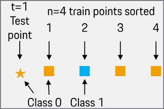
Consider a KNN model with parameter $k=3$, $t=1$ test point denoted $y_{test}$, $n=4$ train points sorted starting from the closest to the test point, $N=\{1,2,3,4\}$, See Figure 1.

$v(N)=2/3$

The calculation of the Shapley values requires training and testing the model with various training sets. In the following examples, we illustrate the calculation of the valuation function for alternative training sets: $u_{y_{test}}(\{1\})=1/3$
$u_{y_{test}}(\{2\})=0/3$
$u_{y_{test}}(\{1,3,4\})=3/3$

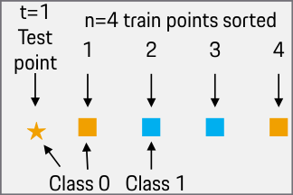
Consider the simple dataset in Figure 2. Let $k=2$ and $N=\{1,2,3,4\}$. To calculate $\phi_{1,2}$, the interaction between $i=1$ and $j=2$, we consider all subsets $S\subseteq N\setminus\{i,j\}$ and calculate the term $\phi_{i,j}$
$v(S\cup\{i,j\})-v(S\cup\{i\})-v(S\cup\{j\})$
For $S=\{3,4\}$:
$v(S\cup\{i,j\})-v(S\cup\{i\})-v(S\cup\{j\})+v(S)=1/2-1/2-0+1/2=1/2$
For $S=\{3\}$: $I=1/2-0-1/2+0=0$
For $S=\{4\}$: $I=1/2-1/2-2/2+1/2=1/2$
For $S=\emptyset$: $I=1/2-0-1/2+0=0$
Finally, $\phi_{ij}(v)=\frac{2}{n}\sum_{S\subseteq N\setminus\{i,j\}}{\frac{1}{\binom{n-1}{s}}(v(S\cup\{i,j\})-v(S\cup\{i\})-v(S\cup\{j\})+v(S))}$ $\phi_{1,2}(v)=\frac{2}{4}(\frac{1}{\binom{4-1}{2}}\frac{1}{2}+0+\frac{1}{\binom{4-1}{1}}\frac{1}{2}+0)=1/6$

The Calculation of the matrix of interactions $\phi_{ij}$, $i\neq j$ is challenging because Equation 3 requires $\mathcal{O}(2^{n})$ trainings of the model, each time over a subset $S\subseteq N$. Therefore, there are no real-world applications at this level [6]. We propose to simplify $\phi_{ij}$ for a specific $v(S)$.

The calculation of the main terms $\phi_{ii}$ can be done in polynomial time and does not represent an issue. For this reason, the focus of this paper is the interaction term $\phi_{ij}$.

Equation 1 involves a linearity relative to the test set: $\phi_{ij}(v)=\frac{1}{t}\sum_{y_{test}\in T}\phi_{ij}(u_{y_{test}})$. Moreover, Equation 2 is linear for train sets of size $s\leq k$, which would allow simplifying the Shapley Interaction equation.

In the following sections, we will use $u_{y_{test}}(S)$ with only a singleton. Therefore, we simplify the notation by discarding the curved parenthesis. Note that in this specific case, the sum is discarded and the function returns only 0 or $1/k$ to express weather train point $i$ has the same label as test point $y_{test}$.

Consider the valuation function of KNN models defined in Equations 1 and 2. The Shapley-Taylor Interaction index ($\phi_{ij}$) can be calculated recursively using Algorithm 1.

The interaction $\phi_{ij}(u_{y_{test}})$ is independent of point $i$ in the case of one test point (demonstrated in Equation 8). This is explained by the fact that KNN does not consider each point individually, but it considers only the order in which the train points come. Nevertheless, once we average over multiple test points, $\phi_{ij}$ becomes dependent on both $i$ and $j$.

Choosing to work with KNN as a surrogate model did speed up the computation. But, on the other hand, it did introduce another parameter: $k$. We prove that, in practice, $k$ does not change the overall shape of the interaction matrix. We conduct an empirical experiment based on 16 simple datasets described in Appendix 0.C. We consider the following range for the $k$ parameters: $3\leq k\leq 20$. For each $k_{1},k_{2}$ in the selected range, we find that the Pearson’s correlation between the two STI-KNN matrices is each time higher than $0.99$. This involves an insignificant change between pair-interaction matrices. Moreover, visual comparison of the matrices does not reveal any difference, see Appendix 0.B.

$n$ is the training set size. $t$ is the testing set size. The complexity of the function STI-KNN-one-test (1), is $\mathcal{O}(n^{2})$ because, first, it sorts the training points in $\mathcal{O}(n\log{}n)$ (2), second, it calculates recursively the super-diagonal in $\mathcal{O}(n)$(4), and third it repeats the values in $\mathcal{O}(n^{2})$. The main script loop through the testing set and apply the function in $\mathcal{O}(tn^{2})$ (18), then it averages over the list of matrices by reducing the dimensions from (n,n,t) to (n,n) which costs $\mathcal{O}(tn^{2})$ (21). Thus, the complexity is $\mathcal{O}(tn^{2})$.

i.e., $mean(\{\phi_{ij}\})\approx 0$

The obtained result for STI could be applied to SII [4], a similar pair interaction algorithm. The only difference would be in the coefficient. For example for SII: $\phi_{n-1,n}(u_{y_{test}})=-\frac{1}{n-1}u_{y_{test}}(\alpha_{n})$.

We further discuss the visual interpretation of the STI-KNN matrix in Section 4.

References

- [1] Gholamy, A., Kreinovich, V., Kosheleva, O.: Why 70/30 or 80/20 relation between training and testing sets: A pedagogical explanation (2018)
- [2] Ghorbani, A., Abid, A., Zou, J.: Interpretation of neural networks is fragile. In: Proceedings of the AAAI conference on artificial intelligence. vol. 33, pp. 3681–3688 (2019)
- [3] Ghorbani, A., Zou, J.: Data shapley: Equitable valuation of data for machine learning. In: International Conference on Machine Learning. pp. 2242–2251. PMLR (2019)
- [4] Grabisch, M., Roubens, M.: An axiomatic approach to the concept of interaction among players in cooperative games. International Journal of game theory 28, 547–565 (1999)
- [5] Jia, R., Dao, D., Wang, B., Hubis, F.A., Gurel, N.M., Li, B., Zhang, C., Spanos, C.J., Song, D.: Efficient task-specific data valuation for nearest neighbor algorithms. arXiv preprint arXiv:1908.08619 (2019)
- [6] Jia, R., Wu, F., Sun, X., Xu, J., Dao, D., Kailkhura, B., Zhang, C., Li, B., Song, D.: Scalability vs. utility: Do we have to sacrifice one for the other in data importance quantification? In: Proceedings of the IEEE/CVF Conference on Computer Vision and Pattern Recognition. pp. 8239–8247 (2021)
- [7] Kwon, Y., Zou, J.: Beta shapley: a unified and noise-reduced data valuation framework for machine learning. arXiv preprint arXiv:2110.14049 (2021)
- [8] Pedregosa, F., Varoquaux, G., Gramfort, A., Michel, V., Thirion, B., Grisel, O., Blondel, M., Prettenhofer, P., Weiss, R., Dubourg, V., et al.: Scikit-learn: Machine learning in python. the Journal of machine Learning research 12, 2825–2830 (2011)
- [9] Shapley, L.: Quota solutions op n-person games1. Edited by Emil Artin and Marston Morse p. 343 (1953)
- [10] Sundararajan, M., Dhamdhere, K., Agarwal, A.: The shapley taylor interaction index. In: International conference on machine learning. pp. 9259–9268. PMLR (2020)
- [11] Xiao, H., Rasul, K., Vollgraf, R.: Fashion-mnist: a novel image dataset for benchmarking machine learning algorithms. arXiv preprint arXiv:1708.07747 (2017)
- [12] Yoon, J., Arik, S., Pfister, T.: Data valuation using reinforcement learning. In: International Conference on Machine Learning. pp. 10842–10851. PMLR (2020)
Appendix 0.A Lemmas and Proof of Section 3.1
Algorithm 1 is composed of three main equations (Equations 6, 7 and 8). The proof is divided into three subsections demonstrating each of these three main equations. Figure 6 summarizes the flow of the proofs involving all lemmas and equations.
Simplify notations
In the following, we simplify unions between sets by writing for example rather than . Without loss of generality, we suppose that train data points are sorted starting from the closest to . Sorted train data points were denoted . But we simplify the notation to . Finally, since in all demonstrations, we will work with the function from Equation 5, we simplify its notation to .
0.A.1 Proof of the last term
The proof of Algorithm 1 starts with the Proof of Equation 10.
Lemma 1 (STI Equation with restricted double sum)