Real-time 6K Image Rescaling with Rate-distortion Optimization
Abstract
Contemporary image rescaling aims at embedding a high-resolution (HR) image into a low-resolution (LR) thumbnail image that contains embedded information for HR image reconstruction. Unlike traditional image super-resolution, this enables high-fidelity HR image restoration faithful to the original one, given the embedded information in the LR thumbnail. However, state-of-the-art image rescaling methods do not optimize the LR image file size for efficient sharing and fall short of real-time performance for ultra-high-resolution (e.g., 6K) image reconstruction. To address these two challenges, we propose a novel framework (HyperThumbnail) for real-time 6K rate-distortion-aware image rescaling. Our framework first embeds an HR image into a JPEG LR thumbnail by an encoder with our proposed quantization prediction module, which minimizes the file size of the embedding LR JPEG thumbnail while maximizing HR reconstruction quality. Then, an efficient frequency-aware decoder reconstructs a high-fidelity HR image from the LR one in real time. Extensive experiments demonstrate that our framework outperforms previous image rescaling baselines in rate-distortion performance and can perform 6K image reconstruction in real time.
1 Introduction

| Method | (a) Downsampled JPEG + super-resolution lim2017enhanced | (b) Flow-based rescaling xiao2020invertible; liang2021hierarchical | (c) Ours |
|---|---|---|---|
| Architecture | |||
| Reconstruction fidelity | ✗ | ✓ | ✓ |
| Rate-distortion optimization | ✗ | ✗ | ✓ |
| Real-time 6K reconstruction | – | ✗ | ✓ |
With an increasing number of high-resolution (HR) images being produced and shared by users on the internet, a new challenge has arisen: how can we store and transfer HR images efficiently? Storing HR images on the cloud, such as iCloud, is becoming a widely adopted solution that saves storage on a user’s mobile device (e.g., smartphones) as only their low-resolution (LR) counterparts are stored on the mobile device for an instant preview. However, when a user wants to obtain the full-resolution image, the entire HR image must be downloaded on the fly from the cloud, which can result in a poor user experience when the internet connection is unstable or not available.
Real-time image rescaling can serve as a competitive solution to improving the user experience of cloud photo storage, as shown in Fig. 1. Such a solution can first embed an HR image (on the cloud) into an LR JPEG thumbnail (on the mobile device) by an encoder, and the thumbnail provides an instant preview with little storage. When the user wants to zoom in on the thumbnail, the HR image with fine details can be reconstructed locally in real time. In addition, image rescaling has other applications in image sharing, as it can “bypass” the resolution limitation of some platforms (e.g., WhatsApp) to reconstruct a high-quality HR image from an LR one xing2022scalearbitrary. While modern smartphones and cameras can capture ultra-high-resolution images in 4K (iPhone 13) or even 6K (Blackmagic camera), we are interested in designing a real-time image rescaling framework for ultra-high-resolution images (e.g., 4K or 6K), which minimizes LR file size while maximizing HR and LR image quality.
However, existing image rescaling methods have their own flaws in practice, as shown in Table 1 where we compare different image rescaling methods in terms of their properties. One potential solution is to upsample the downsampled thumbnail with super-resolution (SR) methods dong2016image; lim2017enhanced; zhang2018residual; zhang2018image; dai2019second; liang2021swinir (Table 1(a)). However, such a framework applies a simple downsampling strategy (e.g., Bilinear, Bicubic) to the HR image so that high-frequency details are basically lost in the LR thumbnail. Also, SR methods only focus on HR reconstruction, which leads to a sub-optimal image rescaling performance. Instead, dedicated image rescaling approaches aim to embed information into a visually pleasing LR image and then reconstruct the HR image with an upsampling module. Recently, state-of-the-art image rescaling works utilize normalizing flow xiao2020invertible; liang2021hierarchical; huang2021video; xing2022scalearbitrary show impressive image embedding and reconstruction capability that outperforms SR approaches, in terms of the reconstructed HR image quality. However, there are still some great challenges to apply these flow-based rescaling frameworks in real-world applications, as shown in Table 1(b). First, the file size of the LR thumbnail is not optimized. Second, the reconstruction stage of these image rescaling methods is computationally expensive due to their invertible network architecture with extensive use of dense blocks huang2017densely: IRN xiao2020invertible costs about a second to reconstruct a 4K image with 4x rescaling on a modern GPU, which is far from real time (Table 2).
In this work, we propose the HyperThumbnail, a rate-distortion-aware framework for 6K real-time image rescaling, as shown in Table 1(c). In this framework, we embed an HR image into a low-bitrate JPEG thumbnail by an encoder and a quantization table predictor, as JPEG is a dominant image compression format today JPEGUsageStatistics. Then the JPEG thumbnail can be upscaled to its high-fidelity HR counterpart with our efficient decoder in real time. We leverage an asymmetric encoder-decoder architecture, where most computation is put in the encoder to keep the decoder lightweight. This makes it possible for our decoder to upscale a thumbnail to 6K in real time, significantly faster than previous flow-based image rescaling methods xiao2020invertible; liang2021hierarchical.
Meanwhile, the Rate-Distortion (RD) performance is an important and practical metric rarely studied in prior rescaling works. In this paper, we define the rate as the ratio between the thumbnail file size and the number of pixels in the HR image, also known as the bits-per-pixel (bpp). The distortion consists of two parts: the perceptual quality of the thumbnail (LR distortion) and the fidelity of the restored HR image (HR distortion). The rate-distortion performance evaluates an image rescaling framework in both storage cost and visual quality. Without explicit RD constraints, recent works in image rescaling xiao2020invertible; liang2021hierarchical do not consider RD performance in their models. While some works wu2021embedding; xing2021invertible; jiang2018end; son2022enhanced; xiao2023invertible leverage the rate constraint by embedding extra information in JPEG, they simply utilize a fixed differentiable JPEG module, which we argue is sub-optimal for image rescaling. Because such a process deteriorates the information in the embedding images without considering their local distribution. Moreover, the quantization process of JPEG introduces noise in the frequency domain and introduces well-known JPEG artifacts, which brings great challenges to information restoration.
To remedy these issues, our image rescaling framework is designed to jointly optimize image quality and bpp with entropy models. Instead of using fixed quantization tables in conventional JPEG (Sec. 3.1), we propose a novel quantization prediction module (QPM) that predicts image-adaptive quantization tables, which can optimize RD performance. We further adopt a frequency-aware decoder which alleviates JPEG artifacts in the thumbnails and improves HR reconstruction. Moreover, our asymmetric encoder-decoder framework can be extended to optimization-based compression.
Our contributions are summarized as follows:
- •
We propose a 6K real-time rescaling framework with an asymmetric encoder-decoder architecture, named HyperThumbnail, which embeds a high-resolution image into a JPEG thumbnail that can be viewed in popular browsers. The decoder utilizes both spatial and frequency information to reconstruct high-fidelity images in real time for 6K image upsampling.
- •
We introduce a new quantization prediction module (QPM) that improves the RD performance in the encoding stage of our framework. Furthermore, we adopt rate-distortion-aware loss functions along with QPM to optimize the RD performance.
- •
Experiments show that our framework outperforms state-of-the-art image rescaling methods with higher LR and HR image quality and faster reconstruction speed at similar file size.
2 Related Work
2.1 Image Super-resolution
Image super-resolution (SR) targets at restoring HR images from LR images. Pioneering works on SR such as SRCNN dong2016image, EDSR lim2017enhanced, and other successors zhang2018residual; zhang2018image; dai2019second; li2020lapar; li2022mulut exploit deep neural networks to solve the challenges in image SR. Recently, Liang liang2021swinir propose a Swin Transformer-based framework with state-of-the-art image SR performance. In addition, Wang wang2018esrgan; wang2021real extend SRGAN ledig2017srgan and demonstrate the potential of producing perceptually pleasing HR images with a GAN-based generator. Despite great recent progress, most of these methods assume a simple deterministic downsampling process (e.g., Bicubic downsampling mitchell1988reconstruction), which limits the reconstruction quality of high-frequency details in image SR.
2.2 Image Rescaling
Different from SR, image rescaling aims to downsample the given HR image into a visually satisfying LR image with embedded information, and then reconstruct the HR image with high fidelity. A straightforward solution is downscaling using detail-preserving methods kopf2013content and upscaling with heavy SR networks lim2017enhanced; dai2019second; liang2021swinir. Recently, efforts have been made to apply invertible neural network (INN) to image rescaling. INN dinh2015nice; dinh2017density; kingma2018glow; kumar2019videoflow; grathwohl2019ffjord; behrmann2019invertible; chen2019residual; ouyang2022restorable provides direct access to the inverse mapping of the forward function, making it a popular framework for image rescaling xiao2020invertible; liang2021hierarchical; cheng2021iicnet. Xiao xiao2020invertible make the first attempt to model image downscaling and upscaling using invertible transformation. Liang liang2021hierarchical further formulate the high-frequency components in INNs as a conditional distribution on LR image. However, the equivalence in the computational cost of the encoding and decoding process of INN makes it almost impossible to optimize the backward inference time independently, which limits its practicality in latency-aware scenarios. Besides, the file size of the embedding LR image in existing rescaling frameworks is yet to be studied. In this paper, we leverage the RD metric to evaluate the rescaling methods from a real-world perspective and compare our framework with existing image rescaling models in terms of their bpp and restored HR fidelity.
2.3 Image Compression
Instead of only shrinking the image size spatially, image compression approaches optimize the RD performance by first producing a compact bitstream, then decoding HR from the bitstream. Recently, learning-based methods balle2017end; rippel2017real; balle2018variational; agustsson2019generative; minnen2018joint; toderici2017full; xie2021enhanced; kim2022joint; he2022elic; lee2022dpict have improved RD performance by a large margin with neural encoders and decoders. However, these methods have not been widely adopted on the internet due to issues related to software compatibility or runtime efficiency. If users of neural compression need a thumbnail for easier manipulation and preview, they need to save another redundant file besides the bitstream, which is inconvenient and takes extra storage. Thus, traditional compression algorithms (e.g., JPEG wallace1991jpeg) are still popular on most social media platforms JPEGUsageStatistics.
In this work, we embed HR images into LR JPEG thumbnails and restore HR images with a 6K real-time decoder. Training neural networks with the non-differentiable JPEG algorithm is challenging. Previous works approximate JPEG either with the iterative optimization jiang2018end or the differentiable degradation simulator son2022enhanced; zhao2019learning during training, and revert to the conventional JPEG algorithm at test time. However, these methods do not optimize the RD performance in their models. In a concurrent work, Xiao xiao2023invertible extend IRN with a fixed JPEG compression module and an extra JPEG artifact removal module. However, they have not considered the bpp and the reconstruction quality as a joint optimization problem. In this work, we propose a novel differentiable JPEG process with the QPM guided by a bitrate loss for RD performance optimization. Moreover, our real-time decoder reconstructs the HR image from both the spatial and frequency domains of a thumbnail and further improves the reconstruction quality.
3 Method
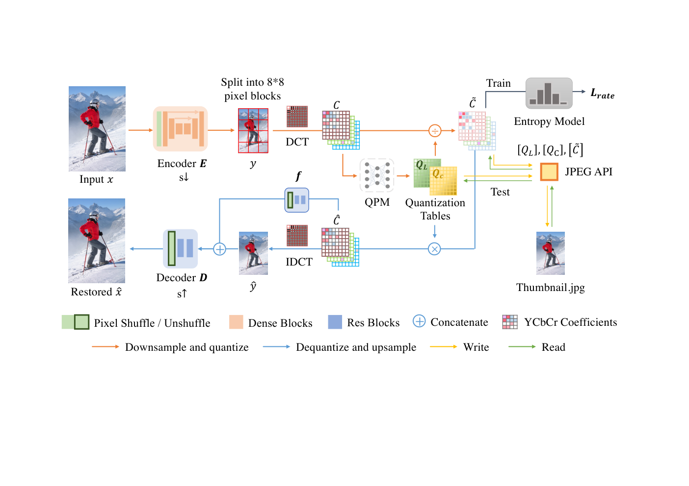 |
3.1 JPEG Preliminary
As our solution involves optimizing the rate-distortion (RD) performance of the JPEG thumbnail, we briefly summarize the JPEG algorithm wallace1991jpeg in this section. The JPEG algorithm compresses an image in three steps. First, given an RGB image , the algorithm converts into the luma-chroma color space (YCbCr). Second, the converted image is divided into pixel blocks as , where . Then, is transformed to its corresponding Discrete-Cosine-Transform (DCT) coefficients :
| (1) |
Third, the luma coefficient and chroma coefficient are quantized separately by two quantization tables and :
| (2) |
where represents the rounding and truncation function. Unlike the original JPEG algorithm which applies a set of image-invariant quantization tables, our work predicts the and with the QPM (Sec. 3.3) for different images. As shown in the bottom-right of Fig. 2, the quantization tables and quantized DCT coefficients are encoded into a JPEG file. At the decoding phase, the JPEG decoder can extract from the JPEG file for image reconstruction with inverted operations of above steps:
| (3) |
and , where IDCT is the inverse operation of DCT, and is the abbreviation of .
3.2 Overview of HyperThumbnail
Inspired by recent progress in high-fidelity efficient restoration through an efficient MLP muller2022instant or a small transformer he2022masked, we adopt an asymmetric encoder-decoder framework, which enables real-time reconstruction. Fig. 2 illustrates the overview of our framework. Given an HR input image , we first generate its LR representation through our encoder , where the is the rescaling factor and our encoder is an U-Net ronneberger2015unet with dense blocks huang2017densely. To further decrease the file size, we transform to DCT coefficients . Then, we quantize with image-specific quantization tables (Sec. 3.3). During the test time, we encode and decode with off-the-shelf JPEG API, and then retrieve with Eqn. (3). In the upsampling stage, we reconstruct the high-fidelity HR with our efficient frequency-aware decoder in real time (Sec. 3.4).
3.3 Quantization Prediction Module
As JPEG wallace1991jpeg is a widely adopted compression algorithm, some previous methods son2022enhanced; jiang2018end; zhao2019learning; xing2021invertible in image embedding also introduce JPEG (Sec. 3.1) to compress their encoded image. However, JPEG degrades the embedded information in the encoded image and leads to a performance drop in the decoding stage (Sec. 5). JPEG uses fixed quantization tables with constant values wallace1991jpeg, which we believe is suboptimal since different images have different frequency distribution. Hence, besides encoding HR images to LR thumbnails, we also predict the quantization tables for each thumbnail with the quantization prediction module (QPM), which boosts the RD performance of our framework significantly. The QPM is implemented as two separate 8-layer multilayer perceptron (MLPs): the luma predictor and the chroma predictor . For block , we vectorize into a 1D vector and produce its quantization table with QPM. Thus we have
| (4) |
where denotes the block counts. To facilitate the conventional JPEG codec, we take the average as the quantization table for the whole image. Following the training stage of learned compression balle2018variational, we adopt the additive uniform noise where each element follows to approximate the non-differentiable quantization noise introduced in Eqn. (2):
| (5) |
In the testing stage, we switch back to the standard quantization function in Eqn. (2) to fit the JPEG API. Experiments show that our QPM predicts better quantization tables so that it improves the RD performance of our framework (Sec. 5). Our experiments in the supplement also show that our QPM improves the standard JPEG algorithm.
3.4 Frequency-aware Decoder
As mentioned in Sec. 3.1, the JPEG quantization is applied on the DCT domain coefficients and leads to the well-known quantization noise. Previous works wu2021embedding; xing2021invertible; son2022enhanced usually decode the embedded information from the RGB domain of the JPEG image. However, we note that quantization noise can be approximated by simple independent uniform noise balle2017end in the DCT domain, but it is nonlinear and more complex to model in the RGB domain after IDCT.
Inspired by recent works in JPEG artifact removal ehrlich2020quantization; wang2016d3; zhang2018dmcnn; guo2016building and image generation nash2021generating, we further propose a novel plug-in named frequency feature extractor for additional frequency domain perception. We first reshape the dequantized DCT coefficients into a sparse representation nash2021generating. Then, we extract features and concatenate with the RGB image . The concatenated features are fed into the decoder to reconstruct the HR image :
| (6) |
where is the concatenation operator along the channel dimension. Since is of in the spatial resolution, takes negligible computational overhead. In this way, our decoder is lightweight enough to reconstruct 6K HR images in real time (Fig. 5). improves our RD performance and is more efficient than increasing the decoder capacity. Please refer to our supplement for more details of our architecture.
3.5 Training Objectives
Bitrate loss To optimize the RD performance of our framework, it is critical to estimate the code length (bitrate) of the quantized coefficients at the training stage. Inspired by Ballé balle2017end, the rate of is estimated with differentiable fully-factorized entropy models:
| (7) |
where and are two fully-factorized entropy models for luma and chroma coefficient maps, respectively. In our work, we reshape to , and assume the value of each pixel in to be independent following Ballé balle2017end. For accurate rate estimation, we train and to model the 64-channel probability density functions of and by minimizing an auxiliary loss balle2018variational. The bpp of the restored image is calculated by
| (8) |
More details of auxiliary loss is provided in the supplement.
Reconstruction and guidance loss Thanks to the fully differentiable pipeline (Fig. 2), it is possible for us to train our encoder, QPM and decoder with similar loss terms used in previous works xiao2020invertible; liang2021hierarchical. Following IRN xiao2020invertible, we employ on the reconstructed and a guidance loss on the JPEG thumbnail :
| (9) | |||||
| (10) |
where is a guidance image downsampled from with bicubic interpolation mitchell1988reconstruction. Altogether, we train our framework by minimizing the total loss :
| (11) |
Empirically, we set . The target bpp of our framework could be adjusted by a loss scaling factor , which we set to for most experiments. The total loss is adopted to optimize the parameters of the encoder, the decoder, and QPM.
| Method | Bitrate-Distortion KodakDataset | Upscaling Efficiency | Reconstructed HR PSNR | |||||||||
|---|---|---|---|---|---|---|---|---|---|---|---|---|
| Down & Degradation & Up | bpp | PSNR | Time (ms) | GMacs | Set5 | Set14 | BSD100 | Urban100 | DIV2K | FiveK-6k | ||
| Bicubic & JPEG & Bicubic | 0.29 | 25.18 | – | – | 25.14 | 23.49 | 24.02 | 21.05 | 25.70 | 26.90 | ||
| Bicubic & JPEG & EDSR lim2017enhanced | 0.29 | 26.77 | 91.0 | 1007.5 | 28.34 | 25.73 | 25.60 | 23.58 | 27.83 | 27.23 | ||
| Bicubic & JPEG & SwinIR liang2021swinir | 0.29 | 26.93 | 4012.6 | 6208.7 | 28.56 | 25.99 | 25.72 | 24.09 | 28.07 | 27.44 | ||
| ComCNN & RecCNN jiang2018end | 0.32 | 27.02 | 469.7 | 6014.7 | 28.29 | 25.84 | 25.78 | 23.70 | 27.99 | 27.40 | ||
| IRN xiao2020invertible & JPEG | 0.31 | 28.48 | 977.8 | 4751.7 | 30.00 | 27.23 | 26.91 | 25.72 | 29.54 | 27.96 | ||
| HCFlow liang2021hierarchical & JPEG | 0.30 | 28.76 | 1025.9 | 4626.0 | 29.98 | 27.41 | 27.05 | 26.19 | 29.71 | 28.01 | ||
| Ours-full | 0.30 | 29.67 | 247.9 | 1277.5 | 30.48 | 28.21 | 27.93 | 27.35 | 30.49 | 28.51 | ||
| Ours | 0.30 | 29.42 | 37.8 | 156.2 | 30.22 | 27.87 | 27.66 | 26.62 | 30.15 | 28.15 | ||
| Ground Truth | IRN xiao2020invertible & JPEG q=96 | HCFlow liang2021hierarchical & JPEG q=90 | Ours | Ours-full |
| \begin{overpic}[figures/section4_experiment/Visual_Comparison/4xresults/0848_GT_cr.png] \put(69.55957,-2.84526){ \includegraphics[width]{figures/section4_experiment/Visual_Comparison/4xlrs/0848LR.png} } \put(79.51802,4.2679){ \includegraphics[width]{figures/section4_experiment/Visual_Comparison/bbox.png}} \end{overpic} | \begin{overpic}[figures/section4_experiment/Visual_Comparison/4xresults/0848IRN_cr.png] \put(69.55957,-2.84526){ \includegraphics[width]{figures/section4_experiment/Visual_Comparison/4xlrs/0848IRN.png}} \put(79.51802,4.2679){ \includegraphics[width]{figures/section4_experiment/Visual_Comparison/bbox.png}} \end{overpic} | \begin{overpic}[figures/section4_experiment/Visual_Comparison/4xresults/0848HCFlow_cr.png] \put(69.55957,-2.84526){ \includegraphics[width]{figures/section4_experiment/Visual_Comparison/4xlrs/0848HCFlow.jpg}} \put(79.51802,4.2679){ \includegraphics[width]{figures/section4_experiment/Visual_Comparison/bbox.png}} \end{overpic} | \begin{overpic}[figures/section4_experiment/Visual_Comparison/4xresults/0848Fast_cr.png] \put(69.55957,-2.84526){ \includegraphics[width]{figures/section4_experiment/Visual_Comparison/4xlrs/0848Fast.jpg}} \put(79.51802,4.2679){ \includegraphics[width]{figures/section4_experiment/Visual_Comparison/bbox.png}} \end{overpic} | \begin{overpic}[figures/section4_experiment/Visual_Comparison/4xresults/0848Full_cr.png] \put(69.55957,-2.84526){ \includegraphics[width]{figures/section4_experiment/Visual_Comparison/4xlrs/0848Full.jpg}} \put(79.51802,4.2679){ \includegraphics[width]{figures/section4_experiment/Visual_Comparison/bbox.png}} \end{overpic} |
| bpp / PSNR(RGB) | 0.324 / 22.82 | 0.296 / 22.47 | 0.240 / 24.32 | 0.238 / 24.78 |
| \begin{overpic}[figures/section4_experiment/Visual_Comparison/4xresults/0888_GT_cr.png] \put(69.55957,-2.84526){ \includegraphics[width]{figures/section4_experiment/Visual_Comparison/4xlrs/0888LR.png}} \put(83.50139,6.54413){ \includegraphics[width]{figures/section4_experiment/Visual_Comparison/bbox.png}} \end{overpic} | \begin{overpic}[figures/section4_experiment/Visual_Comparison/4xresults/0888IRN_cr.png] \put(69.55957,-2.84526){ \includegraphics[width]{figures/section4_experiment/Visual_Comparison/4xlrs/0888IRN.png}} \put(83.50139,6.54413){ \includegraphics[width]{figures/section4_experiment/Visual_Comparison/bbox.png}} \end{overpic} | \begin{overpic}[figures/section4_experiment/Visual_Comparison/4xresults/0888HCFlow_cr.png] \put(69.55957,-2.84526){ \includegraphics[width]{figures/section4_experiment/Visual_Comparison/4xlrs/0888HCFlow.jpg}} \put(83.50139,6.54413){ \includegraphics[width]{figures/section4_experiment/Visual_Comparison/bbox.png}} \end{overpic} | \begin{overpic}[figures/section4_experiment/Visual_Comparison/4xresults/0888Fast_cr.png] \put(69.55957,-2.84526){ \includegraphics[width]{figures/section4_experiment/Visual_Comparison/4xlrs/0888Fast.jpg}} \put(83.50139,6.54413){ \includegraphics[width,trim,clip]{figures/section4_experiment/Visual_Comparison/bbox.png}} \end{overpic} | \begin{overpic}[figures/section4_experiment/Visual_Comparison/4xresults/0888Full_cr.png] \put(69.55957,-2.84526){ \includegraphics[width]{figures/section4_experiment/Visual_Comparison/4xlrs/0888Full.jpg}} \put(83.50139,6.54413){ \includegraphics[width,trim,clip]{figures/section4_experiment/Visual_Comparison/bbox.png}} \end{overpic} |
| bpp / PSNR(RGB) | 0.350 / 25.45 | 0.304 / 25.11 | 0.272 / 25.69 | 0.271 / 26.03 |
4 Experiments
4.1 Experimental Setup
Evaluation metrics We evaluate our upscaling efficiency using running time and multiply-accumulation operations (MACs). We evaluate the quality of our reconstructed and embedding images using the PSNR on RGB channels.
Rescaling methods are developed to embed an HR image into an LR one to reduce file size. However, there is no existing comprehensive evaluation of bitrate for these methods. Following previous compression approaches balle2017end; balle2018variational; xie2021enhanced, we evaluate the RD performance with the HR reconstruction PSNR against bits-per-pixel. Instead of estimating the bitrate from the entropy encoder (Eqn. (7)) during training, we use the real file size of JPEG thumbnails for evaluating the bitrate:
| (12) |
Since there exists a trade-off between image bitrate and fidelity, we visualize the rate-distortion curve of different models during our ablation study.
Datasets We train our model with the widely-used DIV2K agustsson2017ntire image dataset, which contains 800 2K-resolution images in the training set and 100 more in the validation set. From the perspective of rescaling, we test our model on 4 conventional datasets: the Set5 bevilacqua2012low, Set14 zeyde2010single, BSD100 martin2001database, and Urban100 huang2015single. To reveal our real-world performance, we collect first 20 images above 6K resolution (ranked by their bpp) from MIT-Adobe FiveK bychkovsky2011learning as another test set FiveK-6k. In addition, we evaluate the RD performance on Kodak dataset KodakDataset, which is widely adopted in image compression researches begaint2020compressai. The details of the training strategy are provided in the supplement.
4.2 Compare with Baselines
We consider three categories of reconstruction methods as our baselines: (1) downscaling with Bicubic interpolation, compressing with standard JPEG codec, and upscaling with state-of-the-art SR models lim2017enhanced; liang2021swinir; (2) autoencoder using standard JPEG transmission format jiang2018end; (3) rescaling using symmetric invertible neural network xiao2020invertible; liang2021hierarchical and compressing the LR image using standard JPEG codec. For fair evaluation, we improve the RD performance of baselines using standard JPEG compression. We retrain SR models lim2017enhanced; liang2021swinir on LR JPEG compressed images to restore HR images. Besides, we retrain INN baselines xiao2020invertible; liang2021hierarchical and encoder-decoder baselines jiang2018end with a differentiable JPEG module shin2017jpeg. To compare our RD performance against baselines, we constrain their bpp on Kodak dataset to be around 0.3 by adjusting the quality factor of JPEG compression in all baselines. In our supplement, we provide an additional comparison with image compression (e.g., the original JPEG) and rescaling baselines using their original transmission format (e.g., lossless PNG), where our advantage is even larger.
Upscaling efficiency and HR fidelity Table 2 presents the upscaling efficiency of all methods and reconstruction fidelity at around 0.3 bpp. We measure the running time and GMacs of upscaling a 960 540 resolution LR image to a 3840 2160 HR image on an Nvidia RTX 3090 GPU. We use PyTorch implementation with 16 bits floating-point precision for a fair comparison. As shown in Table 2, “Ours” model only costs of the GMacs and of upscaling time compared to HCFlow liang2021hierarchical. We still improve the reconstructed RGB PSNR by 0.61 dB on BSD100 test set with a significantly lower computation.
In addition, we train the “Ours-full” model with a larger decoder. “Ours-full” model achieves higher PSNR that outperforms HCFlow liang2021hierarchical and IRN xiao2020invertible for more than 1.16 dB on Urban100 test set with only of upscaling time. Fig. 3 provides the visual comparison of restored images. From left to right, we show perceptual differences from ground truth, rescaling results of the baselines xiao2020invertible; liang2021hierarchical with JPEG, and our framework. For the first row, our models restore more textures of the glass and the pot lid. Similarly, among all reconstructions in the second row, only our model can recover the details on hair and earmuffs. Besides, the JPEG compression breaks the invertibility of the INN-based rescaling methods liang2021hierarchical; xiao2020invertible, they failed to restore sharp and accurate high-frequency textures in the HR images.
| Bicubic | IRNxiao2020invertible | HCFlowliang2021hierarchical | Ours | Ours-full |
| & JPEG q=96 | & JPEG q=90 | |||
| \begin{overpic}[figures/section4_experiment/Visual_Comparison/4xlrs/comic_LR.png] \put(29.81015,29.81015){ \includegraphics[width,trim,clip]{figures/section4_experiment/Visual_Comparison/bbox.png}} \end{overpic} | \begin{overpic}[figures/section4_experiment/Visual_Comparison/4xlrs/comic_IRN.png] \put(29.81015,29.81015){ \includegraphics[width,trim,clip]{figures/section4_experiment/Visual_Comparison/bbox.png}} \end{overpic} | \begin{overpic}[figures/section4_experiment/Visual_Comparison/4xlrs/comic_HCFlow.jpg] \put(29.81015,29.81015){ \includegraphics[width,trim,clip]{figures/section4_experiment/Visual_Comparison/bbox.png}} \end{overpic} | \begin{overpic}[figures/section4_experiment/Visual_Comparison/4xlrs/comic_Fast.jpg] \put(29.81015,29.81015){ \includegraphics[width,trim,clip]{figures/section4_experiment/Visual_Comparison/bbox.png}} \end{overpic} | \begin{overpic}[figures/section4_experiment/Visual_Comparison/4xlrs/comic_Full.png] \put(29.81015,29.81015){ \includegraphics[width,trim,clip]{figures/section4_experiment/Visual_Comparison/bbox.png}} \end{overpic} |
 |
 |
 |
 |
|
| bpp /PSNR | 0.510 / 26.67 | 0.468 / 17.47 | 0.430 / 27.99 | 0.446 / 27.90 |
| Method | LR thumbnail PSNR | ||||||
|---|---|---|---|---|---|---|---|
| Down & Degradation | Kodak | Set5 | Set14 | BSD100 | Urb100 | DIV2K | FiveK-6k |
| Bicubic & JPEG | 37.72 | 34.41 | 35.79 | 37.43 | 36.64 | 37.14 | 35.14 |
| IRN xiao2020invertible & JPEG | 30.95 | 30.00 | 27.23 | 26.91 | 25.72 | 29.54 | 31.25 |
| ComCNN & RecCNN jiang2018end | 28.00 | 26.76 | 26.47 | 27.47 | 25.57 | 28.15 | 28.99 |
| HCFlow liang2021hierarchical & JPEG | 19.88 | 20.08 | 19.42 | 19.65 | 18.96 | 20.52 | 20.31 |
| Ours-full | 33.21 | 31.86 | 31.76 | 32.44 | 31.01 | 33.32 | 33.99 |
| Ours | 33.55 | 31.96 | 31.93 | 32.90 | 31.16 | 33.62 | 34.24 |
| (a) Encoder | (b) Decoder |
|---|---|
LR qualitative evaluation The visual quality of the LR thumbnails is also important because users preview them directly. Table 3 presents the average LR PSNR of corresponding models, we have the best LR PSNR against INN-based methods. In Fig. 4, we qualitatively compare the visual quality of the thumbnails encoded by rescaling methods. Our method generates LR thumbnails with significantly fewer artifacts without compromising much HR reconstruction quality, please see more analysis in Sec. 5.
4.3 Real-time Inference on 6K Images
Fig. 5 shows our evaluation of the downscaling and upscaling runtime of our framework at multiple resolutions. Noted that we conduct the profiling in half-precision (FP16) mode. Besides, we also converted the trained decoder model from PyTorch to FP16 TensorRT model with torch2trt torch2trt API to further reduce the upscaling time without performance drop in HR reconstruction. As shown in Fig. 5(b), our efficient decoder can upscale an LR thumbnail by in real time at 4K () 70.8 FPS, 5K () 38.8 FPS, or 6K () 31.2 FPS on an RTX 3090 GPU.
| kodim04 / kodim09 | (a) Ours with Fixed JPEG tables, q=85 | (b) Ours with Optimized tables | (c) Ours with QPM kodim04 | (d) Ours with QPM kodim09 |
|---|---|---|---|---|
  |
  |
  |
  |
  |
| bpp / LR / HR: kodim09 | 0.263 / 26.91 / 30.54 | 0.289 / 29.10 / 30.93 | - | 0.246 / 31.03 / 34.34 |
| bpp / LR / HR: kodim04 | 0.251 / 26.96 / 31.35 | 0.276 / 29.17 / 31.71 | 0.240 / 34.38 / 32.03 | - |
4.4 Extension for Optimization-based Rescaling
Since the ground truth HR images are available for downscaling during the test stage, we may further optimize our encoder , QPM, and Entropy model, while fixing the pretrained decoder and feature extractor on the user’s device. As shown in the Table 4, optimization-based rescaling improves the restoration PSNR 0.22dB with a lower bitrate on Set14 dataset.
| Method | Optimization | bpp / HR PSNR | ||
|---|---|---|---|---|
| Architecture | iteration | Kodak | Set5 | Set14 |
| Ours | 0 | 0.301 / 29.42 | 0.379 / 30.23 | 0.359 / 27.74 |
| 100 | 0.307 / 29.55 | 0.377 / 30.36 | 0.347 / 27.96 | |
5 Ablation Study
In this section, we study the effectiveness of our proposed Quantization Prediction Module, designed training loss and architectures on “Ours” model.
Quantization prediction module To examine the effectiveness of our QPM, in Fig. 7, we quantitatively evaluate the RD performance on both the restored HR and the LR JPEG thumbnails of different quantization approaches. For “fixed tables” and “optimized tables”, we initialize the quantization tables following the default JPEG. Particularly, for “optimized tables,” we also optimize the quantization tables at the training stage. We illustrate the curve for each model by adjusting the global quality factor on the quantization tables following JPEG as The target bitrate goes lower when increases. In Fig. 6, we also visualize the quantization tables of different settings. We notice that compared to the corresponding value in the fixed or optimized table, the high-frequency quantization steps in the QPM predicted tables are much smaller and are image-specific, which may introduce less compression on the embedding pattern that is important for HR reconstruction. Consequently, compared to settings with image-invariant quantization, “Ours” model achieves the best quality on the reconstructed and introduces significantly fewer artifacts on the LR thumbnail , which also lowers the filesize of the thumbnails. To further investigate the effectiveness of QPM, we also leverage QPM to improve the RD performance of standard JPEG (without the downscaling and upscaling). Please refer to our supplement for more details.
| (a) RD curve of restored HR image | (b) RD curve of LR thumbnail |
|---|---|
Guidance loss In Fig. 7, we also present the RD curve of the “Ours w/o guidance loss” model trained with . At around 0.4 bpp, removing guidance loss raises the HR PSNR by 0.09dB. However, the PSNR of LR thumbnail drops significantly from 34.1 dB to 13.06 dB. It is unacceptable for user-viewable thumbnails.
Encoder decoder architecture As we study some variants of “Ours” model, we find that improves the quality of both encoded LR thumbnail (0.29 dB) and restored HR image (0.10 dB). Also, adopting is more effective than simply increasing the decoder capacity. Moreover, our study of the encoder capacity reveals that our framework does benefit from a larger encoder. More details are in our supplement.
6 Conclusion
In this paper, we propose a new HyperThumbnail framework that can perform real-time 6K image reconstruction from an LR JPEG thumbnail. We utilize an asymmetric encoder-decoder architecture where the encoder takes most of the computation while the decoder is relatively lightweight for real-time performance. A new quantization prediction module is proposed to optimize the RD performance for image rescaling, which is not studied in prior work. Our framework benefits image sharing and transfer in real-world latency-sensitive applications, such as cloud photo storage and retrieval.
Acknowledgement We express our sincere gratitude to our friends and domain experts, Junming Chen, Yue Wu, and Yu Wang for their invaluable contributions to the design of our project. Additionally, we extend our appreciation to Xiaogang Xu and Xilin Zhang for reviewing and revising the writing.
References
- (1) Kodak lossless true color image suite. http://r0k.us/graphics/kodak/. Accessed: 2022-03-01.
- (2) torch2trt. https://github.com/NVIDIA-AI-IOT/torch2trt. Accessed: 2022-09-19.
- (3) Usage statistics of JPEG for websites. https://w3techs.com/technologies/details/im-jpeg. Accessed: 2022-03-01.
- (4) Eirikur Agustsson and Radu Timofte. NTIRE 2017 challenge on single image super-resolution: Dataset and study. In Proceedings of CVPR Workshops, 2017.
- (5) Eirikur Agustsson, Michael Tschannen, Fabian Mentzer, Radu Timofte, and Luc Van Gool. Generative adversarial networks for extreme learned image compression. In Proceedings of ICCV, 2019.
- (6) Johannes Ballé, Valero Laparra, and Eero P. Simoncelli. End-to-end optimized image compression. In Proceedings of ICLR, 2017.
- (7) Johannes Ballé, David Minnen, Saurabh Singh, Sung Jin Hwang, and Nick Johnston. Variational image compression with a scale hyperprior. In Proceedings of ICLR, 2018.
- (8) Jean Bégaint, Fabien Racapé, Simon Feltman, and Akshay Pushparaja. Compressai: a pytorch library and evaluation platform for end-to-end compression research. arXiv:2011.03029, 2020.
- (9) Jens Behrmann, Will Grathwohl, Ricky T. Q. Chen, David Duvenaud, and Jörn-Henrik Jacobsen. Invertible residual networks. In Proceedings of ICML, 2019.
- (10) Marco Bevilacqua, Aline Roumy, Christine Guillemot, and Marie-Line Alberi-Morel. Low-complexity single-image super-resolution based on nonnegative neighbor embedding. In Proceedings of BMVC, 2012.
- (11) Vladimir Bychkovsky, Sylvain Paris, Eric Chan, and Frédo Durand. Learning photographic global tonal adjustment with a database of input / output image pairs. In Proceedings of CVPR, 2011.
- (12) Tian Qi Chen, Jens Behrmann, David Duvenaud, and Jörn-Henrik Jacobsen. Residual flows for invertible generative modeling. In Advances in NeurIPS, 2019.
- (13) Ka Leong Cheng, Yueqi Xie, and Qifeng Chen. IICNet: A generic framework for reversible image conversion. In Proceedings of ICCV, 2021.
- (14) Tao Dai, Jianrui Cai, Yongbing Zhang, Shu-Tao Xia, and Lei Zhang. Second-order attention network for single image super-resolution. In Proceedings of CVPR, 2019.
- (15) Laurent Dinh, David Krueger, and Yoshua Bengio. NICE: non-linear independent components estimation. In Proceedings of ICLR Workshops, 2015.
- (16) Laurent Dinh, Jascha Sohl-Dickstein, and Samy Bengio. Density estimation using real NVP. In Proceedings of ICLR, 2017.
- (17) Chao Dong, Chen Change Loy, Kaiming He, and Xiaoou Tang. Image super-resolution using deep convolutional networks. IEEE Trans. Pattern Anal. Mach. Intell., 38(2):295–307, 2016.
- (18) Max Ehrlich, Larry Davis, Ser-Nam Lim, and Abhinav Shrivastava. Quantization guided JPEG artifact correction. In Proceedings of ECCV, 2020.
- (19) Will Grathwohl, Ricky T. Q. Chen, Jesse Bettencourt, Ilya Sutskever, and David Duvenaud. FFJORD: free-form continuous dynamics for scalable reversible generative models. In Proceedings of ICLR, 2019.
- (20) Jun Guo and Hongyang Chao. Building dual-domain representations for compression artifacts reduction. In Proceedings of ECCV, 2016.
- (21) Dailan He, Ziming Yang, Weikun Peng, Rui Ma, Hongwei Qin, and Yan Wang. ELIC: efficient learned image compression with unevenly grouped space-channel contextual adaptive coding. In Proceedings of CVPR, 2022.
- (22) Kaiming He, Xinlei Chen, Saining Xie, Yanghao Li, Piotr Dollár, and Ross B. Girshick. Masked autoencoders are scalable vision learners. In Proceedings of CVPR, 2022.
- (23) Gao Huang, Zhuang Liu, Laurens van der Maaten, and Kilian Q. Weinberger. Densely connected convolutional networks. In Proceedings of CVPR, 2017.
- (24) Jia-Bin Huang, Abhishek Singh, and Narendra Ahuja. Single image super-resolution from transformed self-exemplars. In Proceedings of CVPR, 2015.
- (25) Yan-Cheng Huang, Yi-Hsin Chen, Cheng-You Lu, Hui-Po Wang, Wen-Hsiao Peng, and Ching-Chun Huang. Video rescaling networks with joint optimization strategies for downscaling and upscaling. In Proceedings of CVPR, 2021.
- (26) Feng Jiang, Wen Tao, Shaohui Liu, Jie Ren, Xun Guo, and Debin Zhao. An end-to-end compression framework based on convolutional neural networks. IEEE Trans. Circuits Syst. Video Technol., 28(10):3007–3018, 2018.
- (27) Jun-Hyuk Kim, Byeongho Heo, and Jong-Seok Lee. Joint global and local hierarchical priors for learned image compression. In Proceedings of CVPR, 2022.
- (28) Diederik P. Kingma and Prafulla Dhariwal. Glow: Generative flow with invertible 1x1 convolutions. In Advances in NeurIPS, 2018.
- (29) Johannes Kopf, Ariel Shamir, and Pieter Peers. Content-adaptive image downscaling. ACM Trans. Graph., 32(6):173:1–173:8, 2013.
- (30) Manoj Kumar, Mohammad Babaeizadeh, Dumitru Erhan, Chelsea Finn, Sergey Levine, Laurent Dinh, and Durk Kingma. Videoflow: A flow-based generative model for video. arXiv:1903.01434, 2019.
- (31) Christian Ledig, Lucas Theis, Ferenc Huszar, Jose Caballero, Andrew Cunningham, Alejandro Acosta, Andrew P. Aitken, Alykhan Tejani, Johannes Totz, Zehan Wang, and Wenzhe Shi. Photo-realistic single image super-resolution using a generative adversarial network. In Proceedings of CVPR, 2017.
- (32) Jae-Han Lee, Seungmin Jeon, Kwang Pyo Choi, Youngo Park, and Chang-Su Kim. Dpict: Deep progressive image compression using trit-planes. In CVPR, 2022.
- (33) Jiacheng Li, Chang Chen, Zhen Cheng, and Zhiwei Xiong. Mulut: Cooperating multiple look-up tables for efficient image super-resolution. In Proceedings of ECCV, 2022.
- (34) Wenbo Li, Kun Zhou, Lu Qi, Nianjuan Jiang, Jiangbo Lu, and Jiaya Jia. LAPAR: linearly-assembled pixel-adaptive regression network for single image super-resolution and beyond. In Advances in NeurIPS, 2020.
- (35) Jingyun Liang, Jiezhang Cao, Guolei Sun, Kai Zhang, Luc Van Gool, and Radu Timofte. Swinir: Image restoration using swin transformer. In Proceedings of ICCV Workshops, 2021.
- (36) Jingyun Liang, Andreas Lugmayr, Kai Zhang, Martin Danelljan, Luc Van Gool, and Radu Timofte. Hierarchical conditional flow: A unified framework for image super-resolution and image rescaling. In Proceedings of ICCV, 2021.
- (37) Bee Lim, Sanghyun Son, Heewon Kim, Seungjun Nah, and Kyoung Mu Lee. Enhanced deep residual networks for single image super-resolution. In Proceedings of CVPR Workshops, 2017.
- (38) David R. Martin, Charless C. Fowlkes, Doron Tal, and Jitendra Malik. A database of human segmented natural images and its application to evaluating segmentation algorithms and measuring ecological statistics. In Proceedings of ICCV, 2001.
- (39) Fabian Mentzer, George Toderici, Michael Tschannen, and Eirikur Agustsson. High-fidelity generative image compression. In Advances in NeurIPS, 2020.
- (40) David Minnen, Johannes Ballé, and George Toderici. Joint autoregressive and hierarchical priors for learned image compression. In Advances in NeurIPS, 2018.
- (41) Don P. Mitchell and Arun N. Netravali. Reconstruction filters in computer-graphics. In Proceedings of SIGGRAPH, 1988.
- (42) Thomas Müller, Alex Evans, Christoph Schied, and Alexander Keller. Instant neural graphics primitives with a multiresolution hash encoding. ACM Trans. Graph., 41(4):102:1–102:15, 2022.
- (43) Charlie Nash, Jacob Menick, Sander Dieleman, and Peter W. Battaglia. Generating images with sparse representations. In Proceedings of ICML, 2021.
- (44) Hao Ouyang, Tengfei Wang, and Qifeng Chen. Restorable image operators with quasi-invertible networks. In Proceedings of AAAI, 2022.
- (45) Oren Rippel and Lubomir Bourdev. Real-time adaptive image compression. In Proceedings of ICML, 2017.
- (46) Olaf Ronneberger, Philipp Fischer, and Thomas Brox. U-net: Convolutional networks for biomedical image segmentation. In Proceedings of MICCAI, 2015.
- (47) Wenzhe Shi, Jose Caballero, Ferenc Huszar, Johannes Totz, Andrew P. Aitken, Rob Bishop, Daniel Rueckert, and Zehan Wang. Real-time single image and video super-resolution using an efficient sub-pixel convolutional neural network. In Proceedings of CVPR, 2016.
- (48) Richard Shin and Dawn Song. JPEG-resistant adversarial images. In Advances in NeurIPS Workshops, 2017.
- (49) Hanbin Son, Taeoh Kim, Hyeongmin Lee, and Sangyoun Lee. Enhanced standard compatible image compression framework based on auxiliary codec networks. IEEE Trans. Image Process., 31:664–677, 2022.
- (50) George Toderici, Damien Vincent, Nick Johnston, Sung Jin Hwang, David Minnen, Joel Shor, and Michele Covell. Full resolution image compression with recurrent neural networks. In Proceedings of CVPR, 2017.
- (51) Gregory K. Wallace. The JPEG still picture compression standard. Commun. ACM, 34(4):30–44, 1991.
- (52) Xintao Wang, Liangbin Xie, Chao Dong, and Ying Shan. Real-esrgan: Training real-world blind super-resolution with pure synthetic data. In Proceedings of ICCV Workshops, 2021.
- (53) Xintao Wang, Ke Yu, Shixiang Wu, Jinjin Gu, Yihao Liu, Chao Dong, Yu Qiao, and Chen Change Loy. ESRGAN: enhanced super-resolution generative adversarial networks. In Proceedings of ECCV Workshops, 2018.
- (54) Zhangyang Wang, Ding Liu, Shiyu Chang, Qing Ling, Yingzhen Yang, and Thomas S. Huang. D3: deep dual-domain based fast restoration of jpeg-compressed images. In Proceedings of CVPR, 2016.
- (55) Yue Wu, Guotao Meng, and Qifeng Chen. Embedding novel views in a single JPEG image. In Proceedings of ICCV, 2021.
- (56) Mingqing Xiao, Shuxin Zheng, Chang Liu, Zhouchen Lin, and Tie-Yan Liu. Invertible rescaling network and its extensions. Int. J. Comput. Vis., 131(1):134–159, 2023.
- (57) Mingqing Xiao, Shuxin Zheng, Chang Liu, Yaolong Wang, Di He, Guolin Ke, Jiang Bian, Zhouchen Lin, and Tie-Yan Liu. Invertible image rescaling. In Proceedings of ECCV, 2020.
- (58) Yueqi Xie, Ka Leong Cheng, and Qifeng Chen. Enhanced invertible encoding for learned image compression. In Proceedings of ACM MM, 2021.
- (59) Jinbo Xing, Wenbo Hu, and Tien-Tsin Wong. Scale-arbitrary invertible image downscaling. arXiv:2201.12576, 2022.
- (60) Yazhou Xing, Zian Qian, and Qifeng Chen. Invertible image signal processing. In Proceedings of CVPR, 2021.
- (61) Roman Zeyde, Michael Elad, and Matan Protter. On single image scale-up using sparse-representations. In Proceedings of Curves and Surfaces, 2010.
- (62) Xiaoshuai Zhang, Wenhan Yang, Yueyu Hu, and Jiaying Liu. Dmcnn: Dual-domain multi-scale convolutional neural network for compression artifacts removal. In Proceedings of ICIP, 2018.
- (63) Yulun Zhang, Kunpeng Li, Kai Li, Lichen Wang, Bineng Zhong, and Yun Fu. Image super-resolution using very deep residual channel attention networks. In Proceedings of ECCV, 2018.
- (64) Yulun Zhang, Yapeng Tian, Yu Kong, Bineng Zhong, and Yun Fu. Residual dense network for image super-resolution. In Proceedings of CVPR, 2018.
- (65) Lijun Zhao, Huihui Bai, Anhong Wang, and Yao Zhao. Learning a virtual codec based on deep convolutional neural network to compress image. J. Vis. Commun. Image Represent., 63, 2019.
Summary
Appendix A Implementation Details
We implement our model in PyTorch and train on a single Nvidia RTX3090 GPU. In this section, we describe the details of our architecture and training settings.
Network Architecture. Table 5 and Table 6 respectively show details of our encoder and decoder. In Table 5, we describe the architecture of our UNet-based encoder ronneberger2015unet. “PixelUnshuffle 4x” stands for the rearrangement of elements shi2016real which downsamples the HR image by a factor of 4. “3×3, 64, LeakyReLU” denotes a 2d convolution operation of kernel size 3, output channel 64, followed by a LeakyReLU operation. We use the implementation of Residual Dense Block from wang2018esrgan, where ”ResidualDenseBlock-32” refers to a Residual Dense Block with minimum channel 32. We save the produced quantization tables and output coefficients into a single JPEG file using TorchJPEG ehrlich2020quantization. Building blocks are shown in brackets, with the number of blocks stacked. Downsampling is performed at the beginning of the downsampling block using max pooling of stride 2. After the first convolution in the upsampling block, we upsample the decoder feature with Pixel Shuffling Operation. Then, skip connections with the encoder features are conducted.
| Stage | Building Block | Output Size |
|---|---|---|
| Input Downsample | ||
| Downsampling Block1 | ||
| Downsampling Block2 | ||
| Upsampling Block1 | ||
| Upsampling Block2 | ||
| Output layer |
In Table 6, we show the details of our efficient decoder, which is developed based on EDSR lim2017enhanced. We extract features and concatenate with the RGB image . The concatenated features are fed into the decoder to reconstruct the HR image :
| (13) |
where is the concatenation operator along the channel dimension.
| Frequency Feature Extractor | Building Block | Output Size |
|---|---|---|
| Input Convolution | ||
| Residual Convolution Block | ||
| Output Convolution |
| Decoder-full | Building Block | Output Size |
|---|---|---|
| Input Convolution | ||
| RRDB Blocks | ||
| Output Convolution |
Training with Pixel Loss. The model is trained with batch size 16 and patch size in each iteration. The initial learning rate is 2e-4. The learning rate is decayed by for every iterations.
Test-time Fine-tuning during Downscaling. During downscaling stage, we optimize the pre-trained encoder with a fixed pretrained decoder. In the optimization during downscaling, we use full-resolution test images without augmentation as batch size 1 to accelerate optimization. For each image in the test set, we optimize the encoder and QPM for 100 iterations with a learning rate of .
Appendix B Additional Comparison Results
B.1 Comparison with Compression+JPEG
The key difference between our rescaling framework with learned image compression balle2018variational; balle2017end; mentzer2020high is that our HyperThumbnail provides an instant preview that is compatible with existing JPEG codec. However, learned image compression typically requires GPU for decompression using neural networks. For users of learned compression, one practical solution to support instant preview is saving a low-resolution JPEG image as a thumbnail besides compressed bitstream, which we refer to as “Compression+JPEG” framework.
Our rescaling framework has two advantages over the above “Compression+JPEG” solution. (a) First, we embed the high-frequency information into a compact single JPEG file that is easy to deliver. In contrast, the “Compression+JPEG” framework requires two different file formats for preview and compressed bitstreams, which is inconvenient for storage and transmission. (b) Secondly, as evaluated in Table 7, it takes considerable storage for standard JPEG wallace1991jpeg thumbnails to have similar fidelity as our encoded LR thumbnails. We choose Hyperprior balle2018variational and HIFIC mentzer2020high, two state-of-the-art compression methods with a similar running time as ours to build “Compression+JPEG” baseline. Because of information redundency in the bitstream and the JPEG file, “Compression+JPEG” framework takes more storage to achieve comparable LR PSNR and HR PSNR with our result. In summary, our HyperThumbnail provides a compact and succinct representation to support both instant preview and high-frequency reconstruction.
| Method | Bpp of File Format | Bitrate-Distortion Kodak | ||
|---|---|---|---|---|
| Architecture | Bitstream | JPEG | Sum of bpp | LR PSNR / HR PSNR |
| Hyperprior balle2018variational+JPEG | 0.214 | 0.148 | 0.51 | 33.41 / 29.22 |
| HIFIC mentzer2020high+JPEG | 0.172 | 0.148 | 0.32 | 33.41 / 29.35 |
| Ours | - | 0.299 | 0.30 | 33.55 / 29.42 |
B.2 Quantitative comparison with JPEG
In Figure. 8, we provide an additional comparison of our rate-HR-distortion performance with baselines. Previous rescaling methods such as IRN xiao2020invertible in PNG format with different rescaling scale (“IRN+PNG ,”) is even worse than “JPEG” wallace1991jpeg. “IRN+JPEG ” shows that JPEG format with different quality factors boosts the rescaling methods. In contrast, our method is much better than the above three baselines, thanks to our image-specific quantization design.
Another interesting extension of our work is to use QPM as a plug-in to improve the performance of traditional JPEG compression, which is shown by “QPM + JPEG” curve. We set the rescaling factor as , remove our encoder and decoder, and only train our QPM Module as a compression method. An improvement of 0.5dB is observed at most bitrate constraints.
Note that traditional image compression codec, such as JPEG, does not produce an LR embedding as rescaling methods. Thus, their results are only for reference.
B.3 Decoding efficiency comparison with AVIF and JPEGXL.
With no available GPU implementation, we test the decoding efficiency of AVIF (344.8 ms) and JPEG-XL (257.9 ms) on an Intel Xeon Gold 5218 server CPU at 4K resolution and 0.3 bpp. In comparison, our decoder (14.1 ms) is much faster with GPU acceleration. According to a survey JPEGUsageStatistics, the usage statistics of JPEG (77.8%) is much higher than AVIF (¡0.1%). Meanwhile, JPEG-XL will soon be deprecated by Chrome, and some websites (e.g., Twitter and Shopee) use JPEG as the only lossy image file format. Meanwhile, our framework can be integrated into most apps (e.g., Chrome and WhatsApp) without building extra support for transmission and previewing, which is more practical and useful.
| Method | Bitrate-Distortion Kodak | Time(ms) | LR PSNR / HR PSNR | |||
| Architecture | bpp | LR PSNR / HR PSNR | Down / Up | BSD100 | Urb100 | DIV2K |
| Ours w/o | 0.30 | 33.26 / 29.32 | 86.2 / 32.3 | 32.56 / 27.57 | 30.90 / 26.46 | 33.40 / 30.00 |
| Ours- w/o -b22 | 0.30 | 33.24 / 29.27 | 86.2 / 38.6 | 32.51 / 27.63 | 30.89 / 26.69 | 33.48 / 30.09 |
| Ours | 0.30 | 33.55 / 29.42 | 86.2 / 37.8 | 32.90 / 27.66 | 31.16 / 26.62 | 33.62 / 30.15 |
| Ours enc-48 | 0.30 | 33.51 / 29.17 | 63.7 / 37.8 | 32.88 / 27.58 | 31.21 / 26.51 | 33.62 / 30.05 |
| Ours enc-96 | 0.30 | 33.52 / 29.29 | 183.5 / 37.8 | 32.88 / 27.66 | 31.22 / 26.66 | 33.62 / 30.15 |
Appendix C Additional Ablation Study
| (a) Ground truth | (b) Ours | (c) Ours |
| \begin{overpic}[figures/section3_ablation/guide_loss/0LR/kodim17.png] \put(74.52539,-9.93924){ \includegraphics[width,trim,clip]{figures/section3_ablation/guide_loss/1e2/kodim17.png} } \end{overpic} | \begin{overpic}[figures/section3_ablation/guide_loss/1e2/hq_9.png] \put(74.52539,-9.93924){ \includegraphics[width,trim,clip]{figures/section3_ablation/guide_loss/1e2/lr_9.jpg} } \end{overpic} | \begin{overpic}[figures/section3_ablation/guide_loss/0LR/hq_9.png] \put(74.52539,-9.93924){ \includegraphics[width,trim,clip]{figures/section3_ablation/guide_loss/0LR/lr_9.jpg} } \end{overpic} |
Guidance Loss. In Figure.9, we conduct a qualitative ablation study of guidance loss. It demonstrates that guidance loss is crucial to preserve the quality of LR images, without introducing noticeable degradation to HR images.
Frequency-aware Decoder. Because the efficiency of HR reconstruction is important for a better user experience, our decoder architecture has to be succinct and effective. In Table 8, we study the capacity of our decoder with frequency feature extractor . Removing in our framework(“Ours-w/o”) results in a drop in both the HR and LR RD performance. Based on “Ours-w/o”, we increase the residual blocks of the decoder from 16 to 22. “Ours-w/o-b22” takes more upscaling time, but it ends up with a similar HR RD performance with “Ours-w/ f” and a significantly inferior LR RD performance. Since the spatial resolution of quantized coefficients is of the embedding image , the running time of frequency feature extractor only accounts for of the entire decoder. Thus, our frequency feature extractor demonstrates a strong advantage with negligible computation cost.
Asymmetric encoder-decoder. We quantitatively evaluate the influence of the encoder capacity on the RD performance in the bottom two rows of Tab. 8. Based on “Ours”, We adjust the channel of our encoder from 64 to 48 and 96. The experiment shows that our framework benefits from the larger encoder. Since the 96-channel encoder is slower than 64 channel encoder and the improvement is marginal, we set encoder channel to 64 in most of our experiments to ease training.
Also, larger decoders can be applied to the same HyperThumbnail for better reconstruction quality. As shown in the table below, “Ours-large” decoder outperforms “Ours-full” decoder in the PSNR of HR significantly (Tab. 9) with of parameters, sharing the same hyperthumbnails.
| Decoder | Kodak | Set5 | Set14 | BSD100 | Urb100 | DIV2K |
|---|---|---|---|---|---|---|
| Ours-full | 29.67 | 30.48 | 28.21 | 27.93 | 27.35 | 30.49 |
| Ours-large | 29.74 | 30.56 | 28.39 | 28.01 | 27.74 | 30.61 |
C.1 Additional qualitative results
In this section, we visualize more results on the DIV2K agustsson2017ntire validation dataset and the FiveK bychkovsky2011learning dataset. Our model achieves the best balance between the embedding artifacts on LR and the restoration of HR detail. Our approach outperforms baseline methods, especially in texture restoration. All baseline models are trained on the same DIV2K training dataset to fit on guidance LR and target HR . The results are cropped from the original image to ease comparison, please refer to Fig. 10. Also, in Fig. 11, we visualize more rescaling results of real world 6K images with our framework.
| EDSR lim2017enhanced | SwinIR liang2021swinir | IRN xiao2020invertible | HCFlow liang2021hierarchical | Ours | Ours-full | Ground Truth |
| & JPEG q=98 | & JPEG q=98 | & JPEG q=96 | & JPEG q=90 | |||
|
|
|
|
|
|
|
|
 | ||||||
