Gaussian Anamorphosis for Ensemble Kalman Filter Analysis of SAR-Derived Wet Surface Ratio Observations
Abstract
Flood simulation and forecast capability have been greatly improved thanks to advances in data assimilation (DA) strategies incorporating various types of observations; many are derived from spatial Earth Observation. This paper focuses on the assimilation of 2D flood observations derived from Synthetic Aperture Radar (SAR) images acquired during a flood event with a dual state-parameter Ensemble Kalman Filter (EnKF). Binary wet/dry maps are here expressed in terms of wet surface ratios (WSR) over a number of subdomains of the floodplain. This ratio is further assimilated jointly with in-situ water-level observations to improve the flow dynamics within the floodplain. However, the non-Gaussianity of the observation errors associated with SAR-derived measurements break a major hypothesis for the application of the EnKF, thus jeopardizing the optimality of the filter analysis. The novelty of this paper lies in the treatment of the non-Gaussianity of the SAR-derived WSR observations with a Gaussian anamorphosis process (GA). This DA strategy was validated and applied over the Garonne Marmandaise catchment (South-west of France) represented with the TELEMAC-2D hydrodynamic model, first in a twin experiment and then for a major flood event that occurred in January-February 2021. It was shown that assimilating SAR-derived WSR observations, in complement to the in-situ water-level observations significantly improves the representation of the flood dynamics. Also, the GA transformation brings further improvement to the DA analysis, while not being a critical component in the DA strategy. This study heralds a reliable solution for flood forecasting over poorly gauged catchments thanks to available remote-sensing datasets.
Index Terms:
Flooding, hydrodynamics, Data Assimilation (DA), Gaussianity, anamorphosis, Ensemble Kalman Filter (EnKF), Remote Sensing (RS), Synthetic Aperture Radar (SAR), Sentinel-1.I Introduction
In 2021, the Emergency Event Database EM-DAT recorded 432 disastrous events related to natural hazards worldwide, among which flooding dominates with 223 occurrences [1]. Globally, flooding alone is responsible for approximately 40% of all natural disasters [2], and as many as 1.47 billion people—nearly 20% of the world population—are directly exposed to flood risks [3]. As such, flood monitoring and prediction is crucial in terms of cost-to-benefit ratio. The forecast mode is essential for civil and industry protection services, while the hindcast mode allows for damage assessments [4, 5] and flood defense design studies [2, 6]. Early warning and emergency management systems rely on the combination of dense and reliable observing network with numerical models possessing robust forecasting capabilities.
I-A Remote-sensing flood observations
While hydrologic and hydraulic numerical models play an indispensable role in forecast capability, their efficiency is limited by the uncertainties inherently existing in their input data. Such uncertain data includes rainfall, discharge inflow, and geometry of the river and the floodplain, namely bathymetric and topographic errors from utilized Digital Elevation Models (DEM), as well as hydraulic parameter errors due to the calibration of friction coefficients. In this context, DA has emerged as an efficient tool in hydrology to reduce these uncertainties, by combining numerical model outputs with various observations from in-situ gauge measurements and/or from satellite Earth Observations. Indeed, the increasing volume of data from space missions has provided more actors involved in flood management with heterogeneous and relevant satellite data, namely altimetry (e.g. TOPEX/POSEIDON, Jason-1/2/3, SARAL/AltiKa, Sentinel-3, Sentinel-6/Jason-CS, SWOT), optical (e.g. SPOT, LANDSAT-7/8/9, MODIS/VIIRS, Pléiades, Sentinel-2) and Synthetic Aperture Radar (SAR) (e.g. Sentinel-1, TerraSAR-X/TanDEM-X, COSMO-SkyMed, ALOS-2 PALSAR-2, RADARSAT-1/2, ENVISAT ASAR, RISAT-1).
A classical DA approach stands in the assimilation of water surface elevation (WSE) data, either from in-situ gauge measurements, from altimetry satellites, or retrieved from remote-sensing (RS) images using flood edge location information combined with complementary DEM data. Satellite SAR data is particularly advantageous as it allows an all-weather day-and-night global-coverage imagery of continental water, depicted by low backscatter (BS) values resulted from the specular reflection of the incident radar pulses [7]. The assimilation of RS-derived WSE is typically convenient as it deals with a diagnostic variable of the model, yet it can suffer from the lack of precision of high-resolution topographic data as noted in various studies [8, 9, 10, 11]. Nevertheless, many research works have proposed the assimilation of RS-derived WSE as summarized in [12, Table 1]. Most commonly used strategies are similar to that of Giustarini et al. 2011: flood edges are identified on SAR images and integrated with an available DEM to derive the WSE on the floodplain, which are then compared with and/or assimilated to the WSE simulated by 1D or 2D hydrodynamic model to sequentially update the model state and parameters.
The need to retrieve WSE from flood extents can be avoided with direct assimilation of SAR-derived flood probability maps or flood extent maps. The assimilation of surface water extents has been presented in large-scale hydrology and in catchment-scale hydrodynamic by various approaches. In [12], daily surface water extents from the so-called Global Flood Detection System are assimilated with an Ensemble Kalman Filter (EnKF) that relies on the random perturbations of the precipitation—input to the distributed hydrological rainfall-runoff LISFLOOD model [13]—with a focus on Africa and South America catchments. At daily time steps, the innovations of streamflow volumes (i.e. the differences between simulated and observed ones) are computed. They are then used by an EnKF algorithm with a state-augmented strategy to correct and update the simulated groundwater levels in the catchment, instead of the simulated streamflow levels, in order to improve streamflow forecasts. It was shown that the assimilation of RS-derived surface water extents greatly improves flood peak forecasting in terms of timing and volume for slow-motion ungauged catchments. Lai et al. 2014 proposed a 4D-Var (four-dimensional variational) DA scheme implemented on top of a 2D Shallow Water model; differentiated with an automatic differentiation tool called TAPENADE [15]; to assimilate flood extent observations derived from MODIS (Moderate-resolution Imaging Spectroradiometer) in order to correct roughness parameters over the floodplain. The assimilation of flood extent data was shown to be suitable for improving flood modeling in the floodplain or similar areas with slowly-varying bed slopes.
While both [12] and [14] strategies rely on the expression of flood extents as a function of the model state, other research works propose a more direct use of SAR observations. Cooper et al. 2019 proposed an observation operator that directly takes into account synthetical SAR BS values as observations, in an Observing System Simulation Experiment (OSSE) framework, in order to circumvent the needed flood extent mapping and flood pixel-wise probability estimation processes. It relies on the assumption that SAR images must yield distinct distributions of wet and dry BS values, which may not hold for real SAR data that may require further treatments, such as hierarchical split-based approach [17]. Hostache et al. 2018 presents the assimilation of ENVISAT ASAR-derived flood probability maps using a Particle Filter (PF) approach with a sequential importance sampling into a coupled hydrologic-hydraulic model. As detailed in [19], such a probabilistic flood map represents the probability of an observed BS value to correspond to a flood pixel, assuming that its prior probability to be flooded or non-flooded are two Gaussian probability density functions (PDF).
I-B Dealing with non-Gaussianity in DA
The non-Gaussianity characteritics of SAR-derived observation errors need to be properly accounted for in the framework of DA. Indeed, the optimality of the KF and variational analysis relies on the Gaussian assumption for the background and observation errors, as well as on the linearity of the observation operator that relates the control and the observation spaces [20]. When these assumptions no longer hold, the KF or variational analysis can still be used but they are suboptimal. As such, when the Gaussianity assumptions are strongly violated, a pre-processing step is necessary.
For instance, Neal et al. 2009 proposed an adaptive sampling method that only assimilates the measurements that did not fail the normality test. A classical approach in Numerical Weather Prediction (NWP), yet still questionable for extreme events, consists in rejecting outlier observations with a Quality Control (QC) procedure applied on the innovation (also called misfit), assuming that the non-Gaussianity is entirely attributable to observation errors, as these observations are statistically unlikely and their assimilation may lead to a spurious analysis [22, 23]. The simplest approach is thus to assume that the remaining data is correct and follows a Gaussian distribution, then to apply classical variational DA algorithms. In the context of an operational NWP, the “Gaussian plus flat” distribution is often used as a refinement with a gray zone between correct data and grossly erroneous data [24, 25]. In addition, Tavolato and Isaksen 2015 found that a Huber norm (i.e. Gaussian distribution in the center of the distribution and exponential distribution at the tails) was the most suitable distribution to describe the statistics of the innovations, assuming that the majority of the outliers cannot be considered as gross errors and that they may provide some relevant information. The observation cost function with QC based on the Huber norm relaxes the rejection threshold for large misfits. This allows to keep observations with large innovations in the analysis, which is particularly beneficial for the representation of extreme events.
The non-Gaussianity of the control and/or observation errors can be handled using a DA algorithm that does not require Gaussianity assumptions. For instance, the PF works with the entire probability function, instead of focusing on the first and second moments of the statistics like KF and variational algorithm do. A considerable number of studies advocate for such a solution, working with a PF or with a Bayesian approach to assimilate SAR-derived observations. Indeed, the PF framework used in [8, 9, 18, 26, 27] offers the key advantage of relaxing the assumption that observation errors are Gaussian, and allows to propagating a non-Gaussian distribution through non-linear hydrologic and hydrodynamic models [28]. This makes it better suited for a DA of probabilistic flood maps than the more widely used EnKF [11, 12, 29] or variational approaches [14]. In addition, in the context of an OSSE, Dasgupta et al. 2021b analyzed the impacts of the characteristics of the RS observing network with a PF that assimilates SAR-based probabilistic flood maps into the LISFLOOD-FP hydrodynamic model for a synthetical set-up of a flood event in the Clarence catchment (Australia). They asserted that the location and timing of the SAR images is more important than the revisit interval for flood forecast accuracy. As a follow-up study of [18], Di Mauro et al. 2021 introduced an enhanced PF algorithm with a tempering coefficient that depends on the size of the desired effective ensemble size after the assimilation. This aims to inflate the posterior probability and avoid degeneracy of a PF that assimilates SAR-derived probabilistic flood maps.
I-C Gaussian anamorphosis
A different strategy stands in transforming the distribution of the SAR-derived observations into a Gaussian distribution, compatible with KF-based DA algorithms. This alleviates the need for advanced processes on the PF implementation to avoid ensemble collapse. Such a strategy is reported in the literature as Gaussian Anamorphosis (GA), also known as normal-score transform. GA is a pre-processing step that maps the control and/or observation variables onto a transformed space where the Gaussianity assumption is better fulfilled. GA was proposed by Bertino et al. 2003 and it has been investigated in different works [32], [33], [34], [35]. In most studies, it was applied to state analysis, as opposed to model parameter analysis (which is performed in this present work). It involves transforming the state variables and observations into new variables with Gaussian features, over which the DA analysis is computed. The inverse of the GA transform must then be used to remap the analysis result back onto the original space.
Bertino et al. 2003 presented the application of the EnKF to transformed Gaussian—or anamorphosed—state variables, with the integration of the anamorphosis in the update step of the analysis for an ocean model. In order to deal with the large dimension of the model state, it is assumed that the distribution of the state variables at different locations are identical, thus a homogeneous anamorphosis function is chosen all over the spatial domain. This has been assessed, in OSSE mode, for a simplified 1D ecological model. Two versions of the EnKF are compared, assuming either a Gaussian or a log-normal distribution for the errors on the synthetical measurements and the ecological model variables. The ordinary (or plain) version of the EnKF leads to the negative values for the nutriment, phytoplankton and herbivore concentrations (i.e. the parameters considered in [31]), which should be truncated, thus resulting in repetitive biases and corrections for these variables that lead to undesired artificial spring blooms. The novel GA version of the EnKF with the log-normal transform reduces the spurious “false starts” of spring blooms and leads to more realistic ecological cycles. In continuity of this work, Simon and Bertino 2009 presents the application of such a non-Gaussian extension of the EnKF to perform model state estimations for a 3D coupled ocean physical-ecosystem model that present non-Gaussian and positive variables. They demonstrated, within an OSSE, that the assimilation of anamorphosed synthetical chlorophyll- surface concentration data presents a slight advantage in effectiveness compared to the plain EnKF with a simple post-processing of negative values. This advocates for the use of GA when dealing with similar RS observations. Simon and Bertino 2012 considers dual state-parameter estimation ([36]) in OSSE, with an EnKF for a simplified 1D ocean ecosystem model (continuing from [31]) that presents non-Gaussian and positive variables. It was shown that GA overcomes the limits of the classical EnKF when dealing with positive variables.
Béal et al. 2010 also showed that GA leads to an improved estimation of the 3D state of a coupled physical-biogeochemical ocean model with respect to a classical EnKF approach. Schöniger et al. 2012 promoted the use of GA in the field of hydrogeology for the correction of the subsurface hydrologic state. Indeed, the state vector of a groundwater flow numerical model is typically non-Gaussian in the presence of strong spatial heterogeneity of the hydraulic conductivity field. Drawdown, pressure head, and concentration state are rendered Gaussian with a non-parametric function and the discretized field of log-conductivity, which are parameters to the model, is estimated sequentially with DA. The parameter-only EnKF scheme obliterates the need for a back transformation step on updated transformed state variables; it also guarantees that the simulated state is coherent with the updated parameters in the sense of the model’s governing equations. The merits of GA for parameter estimation with EnKF were demonstrated in OSSE assimilating synthetical drawdown measurements. Also in hydraulic tomography, the authors of [39, 40, 41] describe a normal-score transformed (also named GA) EnKF to generate log-conductivity realizations which are conditional to log-conductivity and/or transient piezometric head data.
Amezcua and van Leeuwen 2014 studied the merits of a joint transformation for the state and observation variables that yields joint Gaussianity in the transformed space for the analysis step of the EnKF. Indeed, when mapping the model state space onto a transformed space with Gaussian properties, the observation operator may become non-linear, thus raising a new issue for the filter. The joint GA transformed is compared to a transformation in the state variable and/or observation space, for the univariate case. This work was carried out over a simple case in which the Bayesian posterior can be obtained analytically. It was demonstrated that, in spite of the various GA strategies, the optimality of the analysis is not reached but the joint transformation outperforms the other strategies as its solution is closer to that of the Bayesian solution.
I-D Scope of the article
The overall objective of the article is to reduce comprehensively the uncertainties in the model parameters, forcing and hydraulic state, and consequently improve the overall flood re-analysis and forecast capability, especially in the floodplain, by assimilating relevant SAR-derived flood observations. This article presents as the subsequent study of [43, 44, 45] that proposes a DA approach to accommodate 2D SAR-derived observations alongside with in-situ water level (WL) time-series within an EnKF framework for the TELEMAC-2D11 1 www.opentelemac.org (T2D) hydrodynamic model [46] of the Garonne Marmandaise catchment (South-west France). Sentinel-1 SAR-derived flood extent maps are expressed in terms of wet surface ratios (WSR) computed as the ratio between the number of wet pixels detected on SAR-derived flood extent maps over the total number of pixels in a subdomain of the floodplain.
The novelty of this article stands in the treatment of the non-Gaussianity of such SAR-derived WSR observations. A dual state-parameter DA strategy [36] is implemented to reduce the uncertainties in the parameters associated with friction coefficients and upstream forcing. The control vector is augmented with a WL state correction that is uniform over a limited number of subdomains in the floodplain. Here the EnKF algorithm is favored and implemented as it allows to stochastically estimate the covariance matrices between the model inputs/parameters and its outputs, without formulating the tangent linear of the hydrodynamic model with respect to its parameters, under the assumption that the errors in the control vector are properly described by a Gaussian distribution. As this property is violated when considering SAR-derived WSR observations, the GA strategy described in [35] is implemented here. As opposed to previously cited studies, our observation variables may be strictly null (i.e. dry area) or strictly equal to 1 (i.e. totally flooded area). As a consequence, particular efforts were made on the treatment of these extreme values to ensure that the anamorphosis function remains bijective.
The remainder of the article is organized as follows. Section II presents the data that are used in this study. The DA strategy is detailed in Section III with a focus on anamorphosis. Section IV presents the experimental settings for the OSSE and real DA experiments. Section V discusses the merits of the DA and GA strategies for OSSE and real experiments with assessments in the control and observation spaces. Conclusion and perspectives are finally given in Section VI.
II Data
II-A The Garonne Marmandaise catchment and Observations
The study is carried out over a reach of the Garonne River near Marmande for the major flood event that occurred in January-February 2021. The hydrodynamic numerical model T2D is used to simulate and predict the WL (denoted by []) and velocity (denoted by and [] for the two horizontal components) from which flood risk can be assessed. The study case as well as the hydrodynamic model T2D that was set up to represent the dynamics of the flow are fully described in [43, 47]. The major sources of uncertainties are associated with friction coefficients in the riverbed and in the floodplain, the upstream forcing, as well as with the hydraulic state in subdomains of the floodplain. The friction coefficients include six coefficients in the riverbed ( to ) and one in the floodplain , the upstream forcing is corrected by a multiplicative factor , whereas the hydraulic state in subdomains of the floodplain is corrected with a (spatially) uniform WL additive increment to over five subdomains, as illustrated in Figure 1. The a priori values for these aforementioned random variables—their PDF are assumed to be Gaussian—are presented in [43]. The 2021 flood event is of a 20-year return period. Figure 2 depicts available in-situ WL observations, measured every 15 minutes at Tonneins (blue), Marmande (orange) and La Réole (green). The study is carried over a period of 25 days between 2021-01-16 and 2021-02-10 that capture the flood and the recess phases.

Sentinel-1 (S1) [48], carrying a C-band SAR system, with a central frequency of 5.405 GHz. In this work, the Interferometric Wide (IW) mode is used with 250-km-wide swath and a ground resolution of approximately 2022 m, further resampled, reprojected and distributed at 1010 m for the Ground Range Detected (GRD) products. S1 operates as a constellation of two polar-orbiting identical satellites, launched respectively on 2014-04-03 and 2016-04-26, allowing a six-day repeat cycle, until 2021-12-23. The S1 products are used to produce binary water maps with the FloodML software based on a Random Forest Machine Learning algorithm [49, 50]. More details can be found in [47, 51, 52].
The 2021 flood event was observed by twelve S1 images, represented by vertical dashed lines in Figure 2. The flood peak was reached on 2021-02-04 and it exceeded the highest threshold level for flood risk at Marmande set out by the French national flood forecasting center (SCHAPI) in collaboration with the departmental prefect. The validation of the results is also performed using independent observations from relevant high water marks (HWM) dataset. It is a collaborative dataset of collected flood marks22 2 https://www.reperesdecrues.developpement-durable.gouv.fr/ maintained by the local flood forecast services (SPCs) or by the flood risk prevention and management service (GEMAPI) in the floodplain. In the aftermath of the 2021 flood event, 178 HWM observations were collected (accessed in December 2021). It is worth-noting that, due to high cloud cover during this flood event, no Sentinel-2 optical image acquired during the 2021 flood event provides proper observations.
II-B Imperfection in SAR backscatter information
SAR images, like all active coherent imaging systems, suffer from an inherent error called speckle. It is caused by constructive and destructive interference of coherent waves reflected by the many elementary scatterers contained within an imaged resolution cell. It should be noted that, a radiometric and a geometrical correction [53, 54] are classically applied as pre-processing on raw SAR data, so that most of the remaining errors in SAR images lies in speckle errors. In the detected SAR images (intensity or amplitude), the speckle is usually described as a non-Gaussian multiplicative noise. It can be considered as a random variable whose power and magnitude, respectively, follow a negative exponential and a Rayleigh distribution [55]. The inevitable presence of speckles in SAR images makes the image interpretations and analyses particularly difficult. However, their undesirable effects can be reduced with various filtering methods [56, 57, 58]. In addition, multilooking approach also reduces speckle but at the expense of the image spatial resolution. While avoiding such a loss of resolution, adaptive filters also allow for a significant reduction of speckle while better preserving resolution but they alter the statistical properties of the image. Temporal multilooking comes as an interesting solution when image time-series are available. Yet, none of these methods is capable of a complete removal of all speckle in the image [59, 60]. Therefore, the non-Gaussianity of SAR-derived BS observations, more specifically due to speckle, raises major difficulties for image post-processing. As presented in [61], a logarithmic transform can be applied to convert the signal with multiplicative noise into one with additive noise, easier to be treated by analyzing and standard image processing techniques. Once this transform is achieved, the statistical properties of the log-transformed multilook speckle noise are described for further use in SAR image post-processing.
II-C Error in SAR-derived flood observations
As aforementioned, wet pixels on SAR images exhibit low BS since most of the incident radar pulses are specularly reflected away upon arrival at the water surfaces as opposed to dry pixels that exhibit high BS values. While this properties favors the use of S1 images to detect inundated areas, the variability of water roughness and speckle effect may come as a limitation, especially in urban environment or vegetated areas [62, 63].
A number of techniques exist for separating pixels into wet and dry areas based on BS values. Most methods include thresholding [64] with varying levels of user interpretation (as compared in [65]), region growing and clustering [66], and change detection [67]. These techniques can be used to provide observational information for DA frameworks but they have also been used for flood mapping and monitoring (e.g. [8, 65]) as well as for validation and calibration of inundation models [68, 69, 70]. However, uncertainty in flood extent mapping from SAR images, originates from both the input images and the performed classification algorithm. As a result, resulting classification overall accuracy of flooded areas varies considerably and only in rare cases, exceeds 90% [71].

III Methods
III-A Workflow for the DA algorithm
The general framework for DA experimental settings is depicted in Figure 3. Each box represents a step of the DA algorithm, with a multi-layering aspect indicating ensemble steps. The different ensemble inputs, outputs, and variables are represented in white boxes, the observation operators in gray boxes, the T2D model simulations in blue boxes, and the steps conducted in the transformed Gaussian space are represented in red boxes. The real observations are shown in the green block, and the specific steps to generate synthetical observations for the OSSE are gathered in the yellow block on the right-hand side. The blue circles indicate different input choices for the first cycle and for the subsequent ones.
The control vector for the EnKF DA algorithm, has a size up to depending on the DA experimental settings reported in Table I (in Section IV-B). At most, it gathers seven friction coefficients with , one multiplicative parameter to modify the time-varying upstream BC , and five state corrective variables with over the floodplain subdomains. The friction coefficients and multiplicative coefficient for the discharge are constant over a DA cycle and vary from one DA cycle to another.
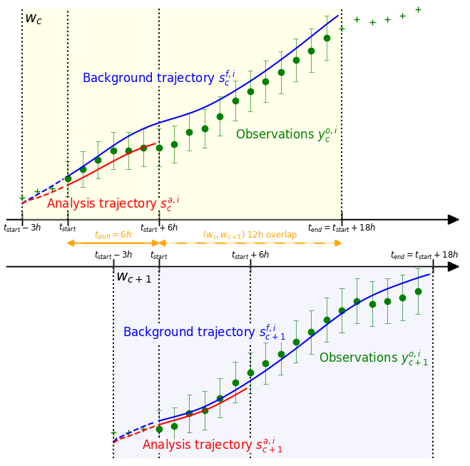
Each DA cycle covers a time window, denoted by over of duration hours over which observations are assimilated, as illustrated in Figure 4. Over each DA cycle , a first simulation with the direct model is carried out—i.e. the background trajectory plotted in blue—and each observation is compared with its model equivalent at the respective observation time over . The observations assimilated over are represented as green circles, whereas the observations that are not assimilated over are depicted as green pluses. The resulting misfit vector is used for the cycle analysis that provides a correction to the control vector. Then, the corrected control vector is used to carry out an analysis trajectory plotted in red, thus providing a coherent updated analyzed hydraulic state. The analysis trajectories are issued over a -hour window starting at in order to allow the hydraulic state to become coherent with the updated parameters and forcing by , and ending at . This provides the final analyzed hydraulic state over for . The cycling of the DA algorithm then consists in sliding the time window of a period hours so that the cycles and overlap for 12 hours. It should be noted that for the very first DA cycle of an event, a 24-hour period of direct simulation (or restart) is achieved before comparing the model outputs to the observations in order to limit the impact of the initial condition.
III-B Description of the EnKF forecast step
The description of the EnKF forecast is detailed in [43, 47]. In the following, indicates the member index within an ensemble of size . (respectively, ) stands for the forecast (respectively, analysis) control vector for member over DA cycle . The EnKF forecast step consists in the propagation in time, over , of the control and model state vectors. These steps are represented in the middle branch of Figure 3. The background hydraulic state for each member results from the integration of the hydrodynamic model : from the control space to the model state (of dimension ) over cycle :
| (1) |
where is a restart file saved from the previous analysis at cycle . As aforementioned, in order to avoid inconsistencies between the state and the analyzed set of parameters at , a short spin-up integration is run on the three hours preceding . The equivalent of the control vector in the observation space is computed with the observation operator : :
| (2) |
The observation vector is noted , it gathers in-situ WL and S1-derived WSR observations for cycle . The in-situ WL subpart of is noted , and the WSR subpart of is noted . The equivalent of results from Eq. 2 that extracts simulated WL at locations and time of in-situ measurements and compute a wet/dry pixel mask from the computed WL simulated 2D field at S1 overpass times in order to compute WSR over each subdomains of the floodplain.
III-C Anamorphosis in the observation space
The step of the DA that relates to the Gaussian anamorphosis are shown in red in Figure 3. The model equivalent of WSR observations is a subset of and is noted in the following. Similarly to the observations , the model equivalent follows a non-Gaussian distribution and is bounded within . In order to prevent the loss of optimality of the EnKF, the GA is applied in the observation space (also called physical space in the following) on the model equivalents and on the observations .
Figure 5 depicts the violin plots of WSR values by aggregating the model equivalents of all SAR-derived WSR observations over the five subdomains of the floodplain from all 75 members of the ensemble, for each S1 overpass time in panel (a) and by aggregating all WSR model equivalents over all the times of S1 for each floodplain subdomain in panel (b), over the entire 2021 flood event. In this Figure, the WSR model equivalents originate from the members of the ensemble of experiment IDA that sequentially assimilates in-situ WL observations at Tonneins, Marmande and La Réole [47]. It appears that, for most dates before the rising limb (2021-02-02) and after the flood peak (2021-02-03), null and small values of WSR prevail as indicated by the flat bottom of the violin plots, whereas higher values of WSR (close to 1) are reached near the flood peak as indicated by the larger flat top of the violin plots. It is worth-noting that for all dates and all floodplain subdomains, the distribution of WSR model equivalents is clearly non-Gaussian.
For a particular cycle , the anamorphosis function is a non-linear bijective function, that maps WSR physical space to a Gaussian space:
| (3) |
This comes down to redefining the observation operator as that now maps the hydraulic state variable onto the transformed space:
| (4) |
where : selects, extracts and eventually interpolates model outputs at times and locations of the in-situ WL observations , whereas it selects, extracts and applies the anamorphosis function at times and locations of WSR observations , over . This corresponds to prescribing an identity function for the anamorphosis of the in-situ WL observations and for that of the WSR observations.
The anamorphosis function is devised from the empirical marginal distribution of the variable in the observation space. For that purpose, all observations in time and space over are taken into account simultaneously. The algorithm to build the anamorphosis function is fully described in [34, Appendix A]. It involves three steps:
- 1.
Construction of the empirical anamorphosis function based on the marginal distribution of the non-Gaussian variable;
- 2.
Interpolation of the empirical piecewise function to allow a bijective function;
- 3.
Definition of the tails of the function necessary to process extremity values.
The first step of the process is widely used in the geostatistical studies and thoroughly detailed in [72]. It maps the sampled values in the physical space onto the Gaussian space. The second and third steps are intended to ensure a bijective function, as presented in [34]. Three different approaches to select relevant samples in the physical space are presented in [35] in the context joint dual state-parameter estimation: (i) a static approach working with existing realizations of the variables to transform; (ii) a dynamic approach: the sample is populated by the members of the forecast ensemble at the time of the analysis; (iii) an hybrid approach: combining both approaches which was shown to be more suitable for the problem of combined state-parameter estimation with non-linear models. In order to build an anamorphosis that is coherent with the flood behavior, the dynamic approach is favored. Nevertheless, it should be noted that the computational cost of the anamorphosis function construction and application is considerably low, given that the size of the ensemble and the observation vectors are small.
The anamorphosis is illustrated in Figure 6 computed by aggregating all WSR model equivalents. The histogram of is shown in Figure 6(a), the devised anamorphosis function is plotted in Figure 6(b) and the histogram of transformed WSR model equivalents is depicted in Figure 6(c). For both Figure 6(a) and Figure 6(c), the cumulative distributions that were used for the function construction are shown in red. In contrast to the eco-biological variables treated in [34, 35], WSR values are likely to reach the bounds of their domain definition, as WSR is strictly equal to 0 for dry areas and to 1 for flooded areas. As a consequence, the tails of the anamorphosis function requires a special treatment in this work to build a bijective function, to ensure a non-null dispersion among the ensemble members and artificially distinguish those all equal to 0 and 1 values—illustrated by the flat bottoms and tops in the violin plots in Figure 5. Indeed, a uniform random noise of small magnitude bounded between and is added to these zeros. These bound values are considered as small with respect to the WSR measurements that lie in , while still significant regarding the numerical precision of our numerical schemes. Similar strategy is also applied for the values close to 1. In the case where the anamorphosis function does not reach the 0 and 1 bounds, the function is extrapolated to cover the whole possible domain of WSR value (green segment of the bijective function shown in Figure 6(b)).
A composite illustration of the GA carried out on one subdomain (e.g. ) at the flood peak (cycle ) is shown in Figure 7. This split-violin plot represents the PDFs of the model equivalents for the WSR observations before GA (represented by the blue area) and after the GA (represented by the green area), using all WSR values from 75 members for the subdomain. It appears, on this example, that the non-Gaussian PDF has been well morphed into a Gaussian PDF. The transformation is carried out centered around the mean of the background WSR values, represented by the green circle, that overlaps with the mean of the transformed distribution (blue circle). The observed WSR value in the physical space (respectively, transformed space) is represented with a white (respectively, red) dot. The prescribed standard deviation for the observation error is indicated by the white (respectively, red) box plot in the physical (respectively, transformed) space. The observation error standard deviation is preserved in the transformed space in this work. An alternative approach using the standard deviation computed based on the transformed variables (performed by [34]) was also tested, but it did not bring any improvement to the DA results. Such a representation extended to all dates and all subdomains of the floodplain is shown in Section V-A.

III-D Description of the EnKF analysis step in the anamorphosed space
The EnKF analysis step usually stands in the update of the control and the associated model state vector , here achieved in the anamorphosed space and represented by a red rectangle in Figure 3. This differs from the classical EnKF analysis [43, 47], as the computation of the innovations and the covariance matrices are achieved in the transformed space using the transformed observation operator :
| (5) |
The Kalman gain is further computed from covariance matrices stochastically estimated within the ensemble, considering anamorphosed observation vectors in place of .
| (6) |
comment equations here to be consistent with the amount of observation given in the forescast step paragraph, and stays different from WRR section
Then, similar to Equation (1), the hydrodynamic state associated with each analyzed control vector results from the integration of the hydrodynamic model with the updated parameters in :
| (7) |
where gathers , and the state correction in the floodplain over , starting from the same initial condition as each background simulation within the ensemble. In should be noted that, in order to preserve a smooth WL field, the mean of the analysis for computed within the ensemble is considered, instead of individual member values.
IV Experimental setting
IV-A Generation of synthetical observations for OSSE
The OSSE experimental setting here is similar to that described in [43, 44]. It is represented on the right branch in Figure 3, framed in a yellow block. The reference simulation (further denoted as True) is a deterministic simulation with a selected set of time-varying parameters for friction and inflow. The true value for with , and with are set from the results of a previous DA experiment on the real 2021 flood event where in-situ WL observations were assimilated, and then a WL correction is added in the floodplain to account for T2D inability to empty the floodplain. Synthetical in-situ and SAR-derived flood extent observations are generated using the observation operator described in Section III applied to the reference simulation outputs. These observations are further assimilated to retrieve the model parameters from the reference simulation, starting from a priori values.
IV-B Configuration for DA experiments and metric assessment
| Name of the | Observing | Ensemble | Control |
|---|---|---|---|
| experiment | network | size | vector |
| FR | No assim | 1 | - |
| IDAosse/IDA | In-situ WL | 75 | |
| IHDAosse/IHDA | In-situ WL and WSR | 75 | |
| IGDAosse/IGDA | In-situ WL and WSR | 75 |
Table I presents the experimental settings for the free run and for the DA simulations that are devised with different control vector and observing network. It should be noted that FR is not represented in Figure 3 as this simulation does not involve DA and is used only to assess the merits of DA. For both OSSE and real experiments, FR is devised using the observed upstream time-series as forcing, as well as the friction coefficients that result from calibration. There is no state correction in the floodplain in FR. The proposed EnKF approach carried out by DA experiments is represented in Figure 3, where the middle branch represents the forecast step and the left branch is the analysis. The real DA experiments use the same forcing and friction coefficient settings as FR at the first DA cycle, and then involve a sequential correction over the next cycles. They assimilate real in-situ WL and WSR observations, represented as green boxes in Figure 3.
The observing network is composed of in-situ WL observations at the three Vigicrue stations Tonneins, Marmande and La Réole, every 15 minutes, eventually completed with WSR values computed over the five floodplain zones at S1 overpass times. IDA experiment only assimilates in-situ WL observations and the control vector is limited to friction coefficients with and the inflow multiplicative coefficient . The control vector for IHDA is extended to include with . It assimilates the same in-situ WL observations like IDA, as well as WSR observations. Lastly, experiment IGDA is at the core of the present work. It is similar to IHDA but the anamorphosis is applied on the vectors expressed onto the observation space in order to alleviate for the violation of the Gaussian assumption for WSR observations. The analysis for IGDA is thus carried out in the transformed Gaussian space.
The observation error (Section III-C) is set proportional to the value of the in-situ WL observations , while it is prescribed as a scalar fixed value for the WSR observations . As such, the standard deviation of the in-situ WL error is fixed to so that . On the other hand, the standard deviation of the SAR-derived WSR observations is fixed to (and up to depending on how early the observation time within each ). These values stem from the assessment of the FloodML algorithm that provides wet/dry classification results (validated on five test sites all over the world) with an overall accuracy of [47]. All DA experiments where carried out using members. In the following, the subscript is used in the experiment name to distinguish the OSSE mode from the real mode.
The metric employed for 1D assessment is formulated as the root-mean-square error (RMSE) of the WL times-series computed with respect to in-situ WL observations (synthetical or real), over time, at the three observing stations. The metric for 2D assessment is the Critical Success Index (), also known as Intersection-over-Union () for RS-based object segmentation tasks, which formulates the fit between a simulated 2D flood extent and an observed flood extent (synthetical or real) derived from S1 observations and FloodML algorithm [50]. varies from 0% when no common area (i.e. no agreement) is found between the simulated and the observed flood extents, and reach their maximal value of 100% when the prediction perfectly fits the observed flood extents. More details on the formulation of these metrics can be found in [47].
V Results
The impact of the GA on the distribution of the WSR model equivalent is shown in subsection V-A. The results of the DA experiments are shown in the control space (subsection V-B) and the observation space (subsection V-C) for both OSSE and real experiments, using RMSE computed at the observing stations and CSI computed over the whole domain.
V-A Result of GA
Similarly to Figure 7, the split-violin plots in Figure 8 show the PDFs for the model equivalent for the WSR observations for 2021 flood event computed considering all WSR observations over each of the five subdomains of the floodplain (subdomain 1 to 5 illustrated in panel (a) to (e)) for each S1 overpass time (along the -axis), with all 75 members of the ensemble. Here again, it is worth-noting that for all subdomains and all dates, the PDFs in the transformed space are well rendered Gaussian, with the mean of the PDF reaching small values before and after the flood peak and large values (close to 1) near the peak (2021-02-03).
V-B Results in the control space
V-B1 Results for OSSE experiment
Figure 9(a) displays the analyzed parameters from the OSSE experiments.
In the river bed, the assimilation of in-situ WL observations with a classical EnKF in IDA suffices to successfully retrieve the true friction coefficients, however with a lesser success for and . The addition of WSR data in IHDA and IGDA does not bring much of an improvement, except for a slight improvement for near Marmande during the flood recess. For in the floodplain, the dispersion of the results is more visible at the flood peak and afterwards, when the sensitivity of the flow to the floodplain friction is most important. Yet, as the velocity of the flow is relatively small, this sensitivity remains weak. The dispersion of the analysis for and is most likely due to equifinality issues, as the downstream part of the flow is also influenced by previous river segments with and . As previously noted in [43], the in-situ WL observation at Marmande is perfectly efficient at constraining the friction coefficient downstream of the gauging station and the analysis for the multiplicative factor is near to perfect for all three DA experiments. When WSR observations are assimilated at S1 overpass times and the correction for the WL is included in the control vector (for IHDA and IGDA experiments), the analysis for is close to the prescribed values for the reference run. The GA in experiment IGDA tends to yield larger increments (negative values) during the flood recess.
V-B2 Results for real experiment
The analyzed parameters from the different DA experiments in real 2021 flood event are shown in Figure 10(a). For all DA experiments, the analyzed values for the friction coefficients in the river bed and the floodplain remain within physical ranges, even though with more dispersion at the flood peak and during the flood recess where the innovations in real event are larger. The analysis for IDA visibly differs from the results of the other DA experiments that assimilated WSR observations with smaller corrections added to the default values, yet all DA analyses follow similar trends for all the components of the control vector. The analyses on are similar for IDA, IHDA, and IGDA for the whole event. This suggests that the in-situ WLs observed at Tonneins are enough to constraint the multiplicative correction to the inflow and that the use of additional data in the floodplain is not necessary. The GA leads to a slightly different analysis compared to IHDA, with larger WL correction (more negative) than IHDA. In contrast to the OSSE, this assessment of the results in the control space does not allow to quantitatively evaluate the DA experiments, since the true values of the controlled parameters are not known.
V-C Results in the observation space
V-C1 Water levels at observing stations (for OSSE and for real experiment)
.
The comparison of WL resulting from the different FR and DA experiments over the entire simulation duration are shown in Figure 11(a) for the OSSE, and in Figure 11(b) for the real flood event at the three observing stations, namely Tonneins (left panel), Marmande (middle panel) and La Réole (right panel). For each subfigure, the top panel represents the WLs—reference WL in black-dashed lines overlapped by simulated WLs in color solid lines—while the bottom panel represents the misfits between the observed and simulated WL by each experiment (FR in orange, IDA in blue, IHDA in green, and IGDA in red). The RMSE computed over the entire event, for the WL from FR simulation, as well as from IDA, IHDA and IGDA analyses, with respect to the reference WL (or real in-situ WL observations) at the three observing stations is indicated in respective subfigures. It can be noted that all DA experiments succeed in significantly reducing the WL errors compared to those of FR. For all three observing stations, the reduction in RMSE with respect to FR reaches 80-90% with slightly different values between IDA, IHDA, and IGDA. This validates the performance of the DA strategy. Most importantly, it demonstrates that the assimilation of in-situ WL in the river bed suffices to constraint the simulated hydraulic state close to the WL measurements at these gauge stations. The merits of assimilating WSR observation is noticeable, on the other hand, when assessing the dynamics of the floodplain. Similar conclusions are drawn from WL timeseries and RMSE assessment for the 2021 real event presented in Figure 11(b) where RMSEs are computed with respect to gauge stations measurements. As expected, for real event, the DA experiments yield a lesser improvement compared to the OSSE, yet it remains very significant. For instance, the WL RMSE at Marmande is reduced from 39.1 cm (FR) to 7.4 cm (IGDA).
V-C2 WSR in the floodplain
Results for OSSE experiment
Figure 12(a) displays the misfit between the synthetical WSR values computed from the reference simulation (black line) and the WSR computed for FR and DA experiments over the five subdomains of the floodplain (same color code as in Figure 9(a)). Between the beginning of the event and the flood rising limb (around 2021-02-01), the assimilation of WSR has virtually no impact as the water has not yet overflowed the floodplain. The WSR values in the reference and the experiments are thus null or close to zero. Globally speaking, FR tends to underestimate the flooding for the OSSE experiment. The assimilation of in-situ WL data (IDA) allows for a significant improvement of WSR near the flood peak but the flood recess suffers from T2D incapacity to effectively empty the floodplains. The impact of assimilating WSR observations is only visible when the flood starts around 2021-02-01 (when reference WSR values are above zero). Analyzed WSR values are further improved when WSR observations are assimilated at S1 overpass times in the two other DA experiments. Indeed, when WSR observations are assimilated and the correction for the WL is included in the control vector (experiments IHDA and IGDA), the analysis succeeds in retrieving WSR values that are close to the truth at the flood peak and in emptying the flood plain after the peak has passed. The results for IHDA and IGDA are quite similar—although IGDA performs slightly better, especially at the flood peak and during the recess period—arguing that when the Gaussian hypothesis is violated, the EnKF analysis may be suboptimal but remains satisfactory in terms of WSR.
Results for real experiment
Figure 12(b) displays the misfit between the S1-derived WSR at S1 overpass times (black line) and the WSR computed for FR and DA experiments over the five subdomains of the floodplain. For the 2021 event, FR tends to underestimate the extension of the flooding whereas all the DA experiments tend to overflood, especially during the flood recess period. It should be noted that the performance of IDA, which does not benefit from WSR observations (i.e. not assimilated), is not improved compared to that of FR. Indeed, in contrast to FR, IDA mostly lead to overflooding throughout the event. On the other hand, IHDA and IGDA experiments provide improvements, shown by the misfits of WSR for these DA experiments being smaller than those of FR, especially during the flood recess over all subdomains of the floodplain. IGDA brings further noticeable improvement to IHDA when WSR data are the most informative, at flood peak and during the flood recess.
A considerable overprediction in the subdomain 4 and 5 at the first S1 overpass time during the rising limb (2021-02-01 07:00) should be noted for all experiments, in Figure 12(b). At this particular moment (7th vertical line in Figure 2) when the WLs in the riverbed are relatively high, the SAR BS tends to intensify due to the increased soil moisture in the floodplain due to rainfalls and the soil being dampened but not yet flooded. The BS will however decrease later on when the floodplain is flooded. Such a behavior leads to the resulting SAR-derived flood extent map at this date yielding fewer detected wet pixels than expected. This situation will be investigated in future works.
| Truth | FR | IDAosse | IHDAosse | IGDAosse | ||
|---|---|---|---|---|---|---|
|
2021-02-03 19:00 |
flood peak |
 |
 |
 |
 |
 |
|
2021-02-07 07:00 |
falling limb |
 |
 |
 |
 |
 |
| Observed | FR | IDA | IHDA | IGDA | ||
|---|---|---|---|---|---|---|
|
2021-02-03 19:00 |
flood peak |
 |
 |
 |
 |
 |
|
2021-02-07 07:00 |
falling limb |
 |
 |
 |
 |
 |

V-C3 2D validation with contingency maps and scores
Results for OSSE experiment
Figure 13(a) shows the reference flood extent maps (first column) and then the resulting contingency maps and score for FR and DA experiments computed with respect to the reference simulation at the time of the flood peak (2021-02-03 19:00) and during water recess (2021-02-07 07:00). The two red-hatched regions are excluded from the assessments due artificial flooding of the first meander in the Garonne T2D model and unreliable topography near La Réole. In the contingency maps, the correctly predicted pixels as non-flooded and flooded are represented in light blue and in dark blue, respectively. The wet pixels incorrectly predicted as non-flooded (or underprediction) are shown in yellow, whereas the dry pixels incorrectly predicted as flooded (or overprediction) are indicated in red.
The flooding is significantly underestimated by FR at the flood peak, as reflected by the large number of yellow underprediction pixels in the floodplain. The assimilation of in-situ WL data in IDA () improves the dynamics of the flow compared to FR (). Yet, the assimilation of WSR observations in IHDA and IGDA yields much higher CSI and better flood extent representation, thanks to the extended control vector involving the associated hydraulic state correction. Indeed, the underprediction and overprediction areas in FR are significantly reduced when WSR are assimilated for both illustrated times of the flood. IHDA and IGDA results are quite close at the flood peak (respectively, 97.26% and 96.72%). During the flood recess, as both IHDA and IGDA allow for an effective emptying of the floodplain, the flood extents are significantly reduced and are in better agreement with the synthetical flood extents, whereas IDA struggles to reduce the overprediction areas exhibited in FR (shown by their CSI = 62.47% for FR and CSI = 63.64% for IDA). IHDA and IGDA’s resulting CSIs are improved with respect to that of FR: from for FR to for IHDA and for IGDA. This results confirm that, when observations are assimilated in the floodplain, the GA strategy brings an improvement with respect to the classical EnKF, especially when the WSR data are most informative with respect to the imperfect dynamics of the numerical model, namely during the flood recess.
Results for real experiment
Figure 14(a) displays the observed flood extent maps derived from S1 images (first column) and the contingency maps for the 2021 flood event at the flood peak (2021-02-03 19:00) and during recess (2021-02-07 07:00) for every experiment. Similarly to what was observed for OSSE, the assimilation of WSR data brings a significant improvement for the representation of the flood extent with respect to FR and also to IDA. It should first be noted that, as expected, for the real experiment, the CSI scores for all experiments remain smaller than those of the OSSE experiments. Indeed, the numerical model struggles to simulate a flow that is in agreement with the observations in both the river bed and the floodplain. At the flood peak, the assimilation of WSR data in IHDA and IGDA brings a significant improvement over all subdomains with respect to FR, shown by fewer underpredicted pixels. Same conclusions are drawn during the flood recess. Indeed, IGDA outperforms IHDA even though some overpredicted areas still remain. These results confirm the merits of assimilating WSR observations, along with the GA step in the DA analysis, even in real event configuration that is more challenging the OSSE configuration.
V-C4 Post-event measure validation with High Water Marks observations (only for real experiment)

A validation of the DA strategies with respect to independent data was finally carried out using the collective public datasets of HWM for the 2021 flood event. This allows to evaluate the highest simulated WLs spatially distributed at various points on the river banks and within the floodplain at the flood peak. Figure 15 gathers the scatter plot of observed highest WL (in -axis) and its simulated values (in -axis) from the different experiments. The diagonal 1:1 line represents the perfect simulation scenario. Compared to FR results (shown by orange crosses that underestimated highest WL values at many locations, encircled in violet), DA allows to significantly reduce the misfits between the observed and simulated highest WL. However, similar results are found between IDA, IHDA, and IGDA. Indeed, since this validation only concerns the highest WL throughout the event, the merits of IGDA demonstrated mostly over the flood recess (Figure 14(a)) remain imperceptible with respect to other DA experiments.
VI Conclusion and perspectives
This article presents a follow-up of our previous study [43] where a Gaussian anamorphosis is proposed to deal with the non-gaussiannity of RS observations’ errors. It highlights the merits of a dual state-parameter EnKF, involving the assimilation of SAR-derived flood extents jointly with gauge water-level data. The proposed method has been validated with OSSE experiments and then assessed in hindcast mode with a real flood event for significant flooding over the Garonne Marmandaise catchment. It was shown that the assimilation of in-situ WL data improves the simulation in the river bed but the complementary assimilation of WSR is key to improve the dynamics in the floodplain, especially at the flood peak and during the flood recess when the T2D model alone struggles to dry out the floodplain. The present work emphasizes on the non-Gaussian properties of observations errors associated with the WSR measurements computed over the subdomains of the floodplain. A Gaussian anamorphosis (GA) strategy, previously proposed in the literature to deal with ecological and hydrogeological variables, was adapted here. The GA maps the observation vector and is model equivalent onto a transformed space where the Gaussianity assumption becomes valid. The anamorphosis function is computed based on the ensemble of simulations that yield the model equivalents of the WSR observations. In our case study, the bijectivity of the GA function is not guaranteed as there are many occurrences of either strictly null or unity values of WSR, respectively when the subdomain is entirely dry or flooded. Therefore, the GA function was made bijective by separating the similar values close to the bounds with a negligible random noise, and then by extrapolating the tails of the function between the leftmost or rightmost values to the unreachable bounds when needed. The major findings from our numerical experiments are summarized as follows:
- •
GA succeeds in transforming the non-Gaussian distribution of observation errors into a Gaussian distribution, for each Sentinel-1 overpass time and for each relevant subdomain of the floodplain.
- •
GA, applied in IGDA experiment, leads to slightly better results than the classical EnKF in IHDA, when assimilating both in-situ WL and WSR observations with a dual state-parameter estimation.
These conclusions advocate for using a GA step when possible, but it also demonstrates that while the classical EnKF is sub-optimal in the presence of non-Gaussianity, its analysis still remains valid and reliable.
As a perspective for this work, one may revisit the assumption of a uniform correction of WL within the floodplain subdomains, as well as the definition of these subdomains, in order to allow for a finer correction of the hydraulic state. Thus far, the DA strategy was implemented with a cycled DA algorithm, only issuing forecast for the following DA cycle. The impact of the DA correction should further be investigated in full forecast mode, considering various lead times that exceed the propagation time of the hydraulic network. For that purpose, the characteristics of the time-varying errors in the control vector should be investigated, and the strategy for prescribing the DA correction beyond the end of the assimilation cycle shall be proposed. By default, a persistent correction could be applied, yet it is expected that such a simple approach could struggle to follow the dynamics of the floods, especially when rapidly changing. In order to tackle longer forecast lead times, chaining the hydrodynamics model with a large-scale hydrologic model could be considered. This approach is currently being investigated. In this perspective, the hypothesis on the stationarity of the errors in the elements of the control vector becomes all the more important, yet it may not stand between the assimilation and the forecast periods. Finally, a major perspective for this research work stands in the assimilation of various RS-derived data from SAR (Sentinel-1, TerraSAR-X), optical (Sentinel-2) and altimetry (Sentinel-6, and the recently launched SWOT) images in order to enrich the observation network and better cover different phases of flood events.
Acknowledgment
The authors gratefully thank the Electricité de France (EDF) for providing the TELEMAC-2D model on the Garonne Downstream catchment, and the SCHAPI, SPCs Garonne-Tarn-Lot and Gironde-Adour-Dordogne for providing in-situ data. They also would like to thank R. Hostache (IRD), R. Fjortoft (CNES), and T. Koleck (CNES) for fruitful discussions and advices, and Q. Bonassies (CERFACS) for helping with the manuscript revision.
References
- CRED [2021] CRED, “Disasters in numbers,” Centre for Research on the Epidemiology of Disasters Institute Health and Society – UCLouvain, Technical Report RT-0300, 2021.
- Shah et al. [2018] M. Shah, A. Rahman, and S. Chowdhury, “Challenges for achieving sustainable flood risk management,” Journal of Flood Risk Management, vol. 11, no. S1, pp. S352–S358, 2018. [Online]. Available: https://onlinelibrary.wiley.com/doi/abs/10.1111/jfr3.12211
- Rentschler and Salhab [2020] J. Rentschler and M. Salhab, People in harm’s way: Flood exposure and poverty in 189 countries. The World Bank, 2020.
- Jamali et al. [2018] B. Jamali, R. Löwe, P. M. Bach, C. Urich, K. Arnbjerg-Nielsen, and A. Deletic, “A rapid urban flood inundation and damage assessment model,” Journal of Hydrology, vol. 564, pp. 1085–1098, 2018.
- Pinter et al. [2017] N. Pinter, N. Santos, and R. Hui, “Preliminary analysis of hurricane harvey flooding in harris county,” Retrieved from UC Davis Center for Watershed Sciences, California WaterBlog, Texas, Technical Report, 2017. [Online]. Available: https://californiawaterblog.com/2017/09/01/preliminary-analysis-of-hurricane-harvey-flooding-in-harris-county-texas/
- Begg [2018] C. Begg, “Power, responsibility and justice: a review of local stakeholder participation in european flood risk management,” Local Environment, vol. 23, no. 4, pp. 383–397, 2018. [Online]. Available: https://doi.org/10.1080/13549839.2017.1422119
- Martinis et al. [2015] S. Martinis, C. Kuenzer, and A. Twele, “Flood studies using synthetic aperture radar data,” in Remote Sensing Handbook. CRC Press, 2015, pp. 145–173.
- Matgen et al. [2011] P. Matgen, R. Hostache, G. Schumann, L. Pfister, L. Hoffmann, and H. Savenije, “Towards an automated SAR-based flood monitoring system: Lessons learned from two case studies,” Physics and Chemistry of the Earth, Parts A/B/C, vol. 36, no. 7-8, pp. 241–252, 2011.
- Giustarini et al. [2011] L. Giustarini, P. Matgen, R. Hostache, M. Montanari, D. Plaza, V. Pauwels, G. De Lannoy, R. D. Keyser, L. Pfister, L. Hoffmann et al., “Assimilating SAR-derived water level data into a hydraulic model: a case study,” Hydrology and Earth System Sciences, vol. 15, no. 7, pp. 2349–2365, 2011.
- Hostache et al. [2009] R. Hostache, P. Matgen, G. Schumann, C. Puech, L. Hoffmann, and L. Pfister, “Water level estimation and reduction of hydraulic model calibration uncertainties using satellite SAR images of floods,” IEEE Transactions on Geoscience and Remote Sensing, vol. 47, no. 2, pp. 431–441, 2009.
- García-Pintado et al. [2015] J. García-Pintado, D. C. Mason, S. L. Dance, H. L. Cloke, J. C. Neal, J. Freer, and P. D. Bates, “Satellite-supported flood forecasting in river networks: A real case study,” Journal of Hydrology, vol. 523, pp. 706–724, 2015.
- Revilla-Romero et al. [2016] B. Revilla-Romero, N. Wanders, P. Burek, P. Salamon, and A. de Roo, “Integrating remotely sensed surface water extent into continental scale hydrology,” Journal of hydrology, vol. 543, pp. 659–670, 2016.
- Van Der Knijff et al. [2010] J. Van Der Knijff, J. Younis, and A. De Roo, “Lisflood: a gis-based distributed model for river basin scale water balance and flood simulation,” International Journal of Geographical Information Science, vol. 24, no. 2, pp. 189–212, 2010.
- Lai et al. [2014] X. Lai, Q. Liang, H. Yesou, and S. Daillet, “Variational assimilation of remotely sensed flood extents using a 2-d flood model,” Hydrology and Earth System Sciences, vol. 18, no. 11, pp. 4325–4339, 2014.
- Hascoët and Pascual [2004] L. Hascoët and V. Pascual, “TAPENADE 2.1 user’s guide,” INRIA, Technical Report RT-0300, 2004. [Online]. Available: https://hal.inria.fr/inria-00069880
- Cooper et al. [2019] E. S. Cooper, S. L. Dance, J. García-Pintado, N. K. Nichols, and P. J. Smith, “Observation operators for assimilation of satellite observations in fluvial inundation forecasting,” Hydrology and Earth System Sciences, vol. 23, no. 6, pp. 2541–2559, 2019.
- Chini et al. [2017] M. Chini, R. Hostache, L. Giustarini, and P. Matgen, “A hierarchical split-based approach for parametric thresholding of SAR images: Flood inundation as a test case,” IEEE Transactions on Geoscience and Remote Sensing, vol. 55, no. 12, pp. 6975–6988, 2017.
- Hostache et al. [2018] R. Hostache, M. Chini, L. Giustarini, J. Neal, D. Kavetski, M. Wood, G. Corato, R.-M. Pelich, and P. Matgen, “Near-real-time assimilation of SAR-derived flood maps for improving flood forecasts,” Water Resources Research, vol. 54, no. 8, pp. 5516–5535, 2018.
- Giustarini et al. [2016] L. Giustarini, R. Hostache, D. Kavetski, M. Chini, G. Corato, S. Schlaffer, and P. Matgen, “Probabilistic flood mapping using synthetic aperture radar data,” IEEE Transactions on Geoscience and Remote Sensing, vol. 54, no. 12, pp. 6958–6969, 2016.
- Asch et al. [2016] M. Asch, M. Bocquet, and M. Nodet, Data assimilation: methods, algorithms, and applications. SIAM, 2016.
- Neal et al. [2009] J. Neal, C. Jeffrey, P. Atkinson, and C. Hutton, “Evaluating the utility of the ensemble transform kalman filter for adaptive sampling when updating a hydrodynamic model,” Journal of Hydrology, vol. 375, no. 3-4, pp. 589–600, 2009.
- Isaksen et al. [2010] L. Isaksen, M. Bonavita, R. Buizza, M. Fisher, J. Haseler, M. Leutbecher, and L. Raynaud, “Ensemble of data assimilations at ecmwf,” ECMWF TD technical Memorandum, Technical Report 636, 2010. [Online]. Available: https://www.ecmwf.int/sites/default/files/elibrary/2010/10125-ensemble-data-assimilations-ecmwf.pdf
- Bonavita et al. [2012] M. Bonavita, L. Isaksen, and E. Hólm, “On the use of eda background error variances in the ecmwf 4d-var,” Quarterly journal of the royal meteorological society, vol. 138, no. 667, pp. 1540–1559, 2012.
- Anderson and Järvinen [1999] E. Anderson and H. Järvinen, “Variational quality control,” Quarterly Journal of the Royal Meteorological Society, vol. 125, no. 554, pp. 697–722, 1999.
- Tavolato and Isaksen [2015] C. Tavolato and L. Isaksen, “On the use of a huber norm for observation quality control in the ecmwf 4d-var,” Quarterly Journal of the Royal Meteorological Society, vol. 141, no. 690, pp. 1514–1527, 2015. [Online]. Available: https://rmets.onlinelibrary.wiley.com/doi/abs/10.1002/qj.2440
- Dasgupta et al. [2021a] A. Dasgupta, R. Hostache, R. Ramsankaran, G. J.-P. Schumann, S. Grimaldi, V. R. N. Pauwels, and J. P. Walker, “A mutual information-based likelihood function for particle filter flood extent assimilation,” Water Resources Research, vol. 57, no. 2, p. e2020WR027859, 2021.
- Di Mauro et al. [2021] C. Di Mauro, R. Hostache, P. Matgen, R. Pelich, M. Chini, P. Jan van Leeuwen, N. Nichols, and G. Bloschl, “Assimilation of probabilistic flood maps from SAR data into a coupled hydrologic-hydraulic forecasting model: a proof of concept.” Hydrol. Earth Syst. Sci., vol. 25, pp. 4081–4097, 2021.
- Moradkhani [2008] H. Moradkhani, “Hydrologic remote sensing and land surface data assimilation,” Sensors, vol. 8, no. 5, pp. 2986–3004, 2008.
- Neal and Jeffrey [2007] J. Neal and C. Jeffrey, “Flood inundation model updating using an ensemble kalman filter and spatially distributed measurements,” Journal of Hydrology, vol. 336, pp. 401–415, 2007.
- Dasgupta et al. [2021b] A. Dasgupta, R. Hostache, R. Ramsankaran, G. J.-P. Schumann, S. Grimaldi, V. R. N. Pauwels, and J. P. Walker, “On the impacts of observation location, timing, and frequency on flood extent assimilation performance,” Water Resources Research, vol. 57, no. 2, p. e2020WR028238, 2021.
- Bertino et al. [2003] L. Bertino, G. Evensen, and H. Wackernagel, “Sequential data assimilation techniques in oceanography,” International Statistical Review, vol. 71, no. 2, pp. 223–241, 2003. [Online]. Available: https://onlinelibrary.wiley.com/doi/abs/10.1111/j.1751-5823.2003.tb00194.x
- Zhou et al. [2011] H. Zhou, J. J. Gomez-Hernandez, H.-J. H. Franssen, and L. Li, “An approach to handling non-gaussianity of parameters and state variables in ensemble kalman filtering,” Advances in Water Resources, vol. 34, no. 7, pp. 844–864, 2011.
- Brankart et al. [2012] J.-M. Brankart, C.-E. Testut, D. Béal, M. Doron, C. Fontana, M. Meinvielle, P. Brasseur, and J. Verron, “Towards an improved description of ocean uncertainties: effect of local anamorphic transformations on spatial correlations,” Ocean Science, vol. 8, no. 2, pp. 121–142, 2012.
- Simon and Bertino [2009] E. Simon and L. Bertino, “Application of the gaussian anamorphosis to assimilation in a 3-d coupled physical-ecosystem model of the north atlantic with the enkf: A twin experiment,” Ocean Science (OS), 03 2009.
- Simon and Bertino [2012] ——, “Gaussian anamorphosis extension of the denkf for combined state parameter estimation: Application to a 1d ocean ecosystem model,” Journal of Marine Systems - J MARINE SYST, vol. 89, pp. 1–18, 01 2012.
- Moradkhani et al. [2005] H. Moradkhani, S. Sorooshian, H. V. Gupta, and P. R. Houser, “Dual state–parameter estimation of hydrological models using ensemble kalman filter,” Advances in water resources, vol. 28, no. 2, pp. 135–147, 2005.
- Béal et al. [2010] D. Béal, P. Brasseur, J.-M. Brankart, Y. Ourmieres, and J. Verron, “Characterization of mixing errors in a coupled physical biogeochemical model of the north atlantic: implications for nonlinear estimation using gaussian anamorphosis,” Ocean Science, vol. 6, no. 1, pp. 247–262, 2010.
- Schöniger et al. [2012] A. Schöniger, W. Nowak, and H.-J. Hendricks Franssen, “Parameter estimation by ensemble kalman filters with transformed data: Approach and application to hydraulic tomography,” Water Resources Research, vol. 48, no. 4, 2012.
- Zhou et al. [2012] H. Zhou, L. Li, H.-J. Hendricks Franssen, and J. J. Gómez-Hernández, “Pattern recognition in a bimodal aquifer using the normal-score ensemble kalman filter,” Mathematical Geosciences, vol. 44, no. 2, pp. 169–185, 2012.
- Li et al. [2012] L. Li, H. Zhou, H. J. Hendricks Franssen, and J. J. Gómez-Hernández, “Groundwater flow inverse modeling in non-multigaussian media: performance assessment of the normal-score ensemble kalman filter,” Hydrology and earth system sciences, vol. 16, no. 2, pp. 573–590, 2012.
- Xu et al. [2013] T. Xu, J. J. Gómez-Hernández, H. Zhou, and L. Li, “The power of transient piezometric head data in inverse modeling: An application of the localized normal-score enkf with covariance inflation in a heterogenous bimodal hydraulic conductivity field,” Advances in Water Resources, vol. 54, pp. 100–118, 2013.
- Amezcua and van Leeuwen [2014] J. Amezcua and P. J. van Leeuwen, “Gaussian anamorphosis in the analysis step of the enkf: a joint state-variable/observation approach,” Tellus A: Dynamic Meteorology and Oceanography, vol. 66, no. 1, p. 23493, 2014. [Online]. Available: https://doi.org/10.3402/tellusa.v66.23493
- Nguyen et al. [2022a] T. H. Nguyen, S. Ricci, A. Piacentini, C. Fatras, P. Kettig, G. Blanchet, S. Peña Luque, and S. Baillarin, “Dual State-Parameter Assimilation of SAR-Derived Wet Surface Ratio for Improving Fluvial Flood Reanalysis,” Water Resources Research, vol. 58, no. 11, p. e2022WR033155, 2022, e2022WR033155 2022WR033155. [Online]. Available: https://agupubs.onlinelibrary.wiley.com/doi/abs/10.1029/2022WR033155
- Nguyen et al. [2022b] T. H. Nguyen, S. Ricci, A. Piacentini, C. Fatras, P. Kettig, G. Blanchet, S. P. Luque, and S. Baillarin, “Assimilation of SAR-derived flood observations for improving fluvial flood forecast,” in Proceedings of the 14th International Conference on Hydroinformatics HIC 2022, 2022.
- Nguyen et al. [2022c] T. H. Nguyen, S. Ricci, A. Piacentini, R. Rodriguez Suquet, G. Blanchet, S. P. Luque, and P. Kettig, “Enhancing Flood Forecasting with Dual State-Parameter Estimation and Ensemble-based SAR Data Assimilation,” in Proceedings of the 28th TELEMAC-MASCARET User Conference (TUC2022), 2022, pp. 297–305.
- Hervouet [2007] J.-M. Hervouet, Hydrodynamics of free surface flows: modelling with the finite element method. Wiley Online Library, 2007, vol. 360.
- Nguyen et al. [2022d] T. H. Nguyen, S. Ricci, C. Fatras, A. Piacentini, A. Delmotte, E. Lavergne, and P. Kettig, “Improvement of Flood Extent Representation With Remote Sensing Data and Data Assimilation,” IEEE Transactions on Geoscience and Remote Sensing, vol. 60, pp. 1–22, 2022.
- Torres et al. [2012] R. Torres, P. Snoeij, D. Geudtner, D. Bibby, M. Davidson, E. Attema, P. Potin, B. Rommen, N. Floury, M. Brown et al., “Gmes sentinel-1 mission,” Remote Sensing of Environment, vol. 120, pp. 9–24, 2012.
- Huang et al. [2020] T. Huang, S. Baillarin, A. Altinok, G. Blanchet, J. Hausman, P. Kettig, and S. Shah, “Distributed Machine Learning and Data Fusion for Flood Detection and Monitoring,” in AGU Fall Meeting Abstracts, vol. 2020, Dec. 2020, pp. IN041–09.
- Kettig et al. [2021] P. Kettig, S. Baillarin, G. Blanchet, C. Taillan, S. Ricci, T.-H. Nguyen, T. Huang, A. Altinok, N. T. Chung, G. Valladeau, R. Goeury, and A. Roumagnac, “The sco-flooddam project: New observing strategies for flood detection, alert and rapid mapping,” in 2021 IEEE International Geoscience and Remote Sensing Symposium IGARSS, 2021, pp. 1464–1467.
- Nguyen et al. [2021] T. H. Nguyen, A. Delmotte, C. Fatras, P. Kettig, A. Piacentini, and S. Ricci, “Validation and Improvement of Data Assimilation for Flood Hydrodynamic Modelling Using SAR Imagery Data,” in Proceedings of the 27th TELEMAC-MASCARET User Conference October (TUC2020), 2021, pp. 100–108.
- Peña-Luque et al. [2021] S. Peña-Luque, S. Ferrant, M. C. Cordeiro, T. Ledauphin, J. Maxant, and J.-M. Martinez, “Sentinel-1&2 multitemporal water surface detection accuracies, evaluated at regional and reservoirs level,” Remote Sensing, vol. 13, no. 16, p. 3279, 2021. [Online]. Available: https://doi.org/doi.org/10.3390/rs13163279
- Blacknell et al. [1989] D. Blacknell, A. Freeman, S. Quegan, I. A. Ward, I. Finley, C. J. Oliver, R. G. White, and J. W. Wood, “Geometric accuracy in airborne SAR images,” IEEE Transactions on Aerospace and Electronic Systems, vol. 25, no. 2, pp. 241–258, 1989.
- Small [2011] D. Small, “Flattening gamma: Radiometric terrain correction for SAR imagery,” IEEE Transactions on Geoscience and Remote Sensing, vol. 49, no. 8, pp. 3081–3093, 2011.
- Xie et al. [2002a] H. Xie, L. E. Pierce, and F. T. Ulaby, “Statistical properties of logarithmically transformed speckle,” IEEE transactions on geoscience and remote sensing, vol. 40, no. 3, pp. 721–727, 2002.
- Kuan et al. [1985] D. T. Kuan, A. A. Sawchuk, T. C. Strand, and P. Chavel, “Adaptive noise smoothing filter for images with signal-dependent noise,” IEEE transactions on pattern analysis and machine intelligence, no. 2, pp. 165–177, 1985.
- Lopes et al. [1990] A. Lopes, R. Touzi, and E. Nezry, “Adaptive speckle filters and scene heterogeneity,” IEEE transactions on Geoscience and Remote Sensing, vol. 28, no. 6, pp. 992–1000, 1990.
- Lee et al. [1994] J. S. Lee, L. Jurkevich, P. Dewaele, P. Wambacq, and A. Oosterlinck, “Speckle filtering of synthetic aperture radar images: A review,” Remote Sensing Reviews, vol. 8, no. 4, pp. 313–340, 1994. [Online]. Available: https://doi.org/10.1080/02757259409532206
- Deledalle et al. [2017] C.-A. Deledalle, L. Denis, S. Tabti, and F. Tupin, “Mulog, or how to apply gaussian denoisers to multi-channel SAR speckle reduction?” IEEE Transactions on Image Processing, vol. 26, no. 9, pp. 4389–4403, 2017.
- Abergel et al. [2018] R. Abergel, L. Denis, S. Ladjal, and F. Tupin, “Subpixellic methods for sidelobes suppression and strong targets extraction in single look complex SAR images,” IEEE Journal of Selected Topics in Applied Earth Observations and Remote Sensing, vol. 11, no. 3, pp. 759–776, 2018.
- Xie et al. [2002b] H. Xie, L. E. Pierce, and F. T. Ulaby, “SAR speckle reduction using wavelet denoising and markov random field modeling,” IEEE Transactions on geoscience and remote sensing, vol. 40, no. 10, pp. 2196–2212, 2002.
- Martinis and Rieke [2015] S. Martinis and C. Rieke, “Backscatter analysis using multi-temporal and multi-frequency SAR data in the context of flood mapping at river saale, germany,” Remote Sensing, vol. 7, no. 6, pp. 7732–7752, 2015.
- Pierdicca et al. [2018] N. Pierdicca, L. Pulvirenti, and M. Chini, “Flood mapping in vegetated and urban areas and other challenges: models and methods,” in Flood Monitoring through Remote Sensing. Springer, 2018, pp. 135–179.
- Henry et al. [2006] J.-B. Henry, P. Chastanet, K. Fellah, and Y.-L. Desnos, “Envisat multi-polarized asar data for flood mapping,” International Journal of Remote Sensing, vol. 27, no. 10, pp. 1921–1929, 2006.
- Brown et al. [2016] K. M. Brown, C. H. Hambidge, and J. M. Brownett, “Progress in operational flood mapping using satellite synthetic aperture radar (sar) and airborne light detection and ranging (lidar) data,” Progress in Physical Geography, vol. 40, no. 2, pp. 196–214, 2016.
- Horritt et al. [2001] M. S. Horritt, D. C. Mason, and A. J. Luckman, “Flood boundary delineation from synthetic aperture radar imagery using a statistical active contour model,” International Journal of Remote Sensing, vol. 22, no. 13, pp. 2489–2507, 2001. [Online]. Available: https://doi.org/10.1080/01431160116902
- Hostache et al. [2012] R. Hostache, P. Matgen, and W. Wagner, “Change detection approaches for flood extent mapping: How to select the most adequate reference image from online archives?” International journal of applied earth observation and geoinformation, vol. 19, pp. 205–213, 2012.
- Mason et al. [2009] D. C. Mason, R. Speck, B. Devereux, G. J.-P. Schumann, J. C. Neal, and P. D. Bates, “Flood detection in urban areas using TerraSAR-X,” IEEE Transactions on Geoscience and Remote Sensing, vol. 48, no. 2, pp. 882–894, 2009.
- Di Baldassarre et al. [2009] G. Di Baldassarre, G. Schumann, and P. D. Bates, “A technique for the calibration of hydraulic models using uncertain satellite observations of flood extent,” Journal of Hydrology, vol. 367, no. 3-4, pp. 276–282, 2009.
- Wood et al. [2016] M. Wood, R. Hostache, J. Neal, T. Wagener, L. Giustarini, M. Chini, G. Corato, P. Matgen, and P. Bates, “Calibration of channel depth and friction parameters in the lisflood-fp hydraulic model using medium-resolution SAR data and identifiability techniques,” Hydrology and Earth System Sciences, vol. 20, no. 12, pp. 4983–4997, 2016.
- Schumann et al. [2012] G. J.-P. Schumann, P. D. Bates, G. Di Baldassarre, and D. C. Mason, The Use of Radar Imagery in Riverine Flood Inundation Studies. John Wiley and Sons, Ltd, 2012, ch. 6, pp. 115–140. [Online]. Available: https://onlinelibrary.wiley.com/doi/abs/10.1002/9781119940791.ch6
- Chiles and Delfiner [1999] J.-P. Chiles and P. Delfiner, Geostatistics: modeling spatial uncertainty. John Wiley & Sons, 1999, vol. 497.