Thermal Spread Functions (TSF): Physics-guided Material Classification

When objects are heated through radiation on surface and allowed to cool down, they display characteristic temperature changes. These changes are based on their initial temperature, surface absorption, and heat diffusivity. We inject heat through a small portion on the surface of a material which diffuses throughout the body over time. If we observe a small patch of material in the vicinity of injection, we observe the diffusion - both during the injection phase and during the cooling phase after no external heat is supplied. We call this varying 2D temperature profile as the Thermal Spread Function (TSF) of the material.

We measure the TSF of the material through a Long Wave Infrared (LWIR) thermal camera. We derive diffusivity and an absorption factor from the TSF to characterize the material as these properties are independent of the initial temperature of the object. Our main contributions are the following.

• •

  We first derive a physically accurate model that characterizes the Thermal Spread Functions (TSFs) as a function of initial temperature of the object and an object’s thermodynamic properties.

• •

  We then use a Finite Differences (FD) Method to solve the inverse heat problem for recovering parameters related to diffusion, absorption and emission

• •

  Finally, we design and demonstrate a simple optical setup for non-invasively recovering the thermodynamic properties and using them to classify materials.

Consider the scene shown in Fig. 2 where an object is illuminated by an external heat source. Let $e$ denote the thermal energy density, $\phi$ represent the heat flux (energy per unit time per unit surface area) across the object boundary and $F$ be the heat absorbed per unit time per unit volume. The energy conservation equation can be written as,

$$\frac{\partial e}{\partial t}=-\frac{\partial\phi}{\partial x}+F.$$

(1)

The expression relating thermal energy density and temperature $u(x,t)$ is,

$$e(x,t)=c(x)\cdot\rho(x)\cdot u(x,t),$$

(2)

where $c(x)$ is the specific heat of the material at $x$, and $\rho(x)$ is its density. Fourier’s law of conduction gives a relation between temperature $u(x,t)$ and flux $\phi(x,t)$:

$$\phi=-\sigma_{0}\cdot\frac{\partial u}{\partial x},$$

(3)

where $\sigma_{0}$ represents conductivity of the material. Substituting Equations 2 and 3 into Equation 1, we get,

$$c\cdot\rho\cdot\frac{\partial u}{\partial t}=\frac{\partial}{\partial x}\left(\sigma_{0}\frac{\partial u}{\partial x}\right)+F,$$

(4)

where $F$ is the heat received by the material per unit time per unit volume. Substituting $k=\frac{\sigma_{0}}{c\rho}$ and $\beta=\frac{1}{c\rho}$ we get,

$$\frac{\partial u}{\partial t}=\frac{\partial}{\partial x}\left(k\frac{\partial u}{\partial x}\right)+\beta F,$$

(5)

If we inject heat energy $f=f_{external}$ per unit time per unit volume, and $\epsilon_{hs}=\epsilon_{HeatSource}$ is the material absorptivity for the wavelength corresponding to heat source, then $F=\epsilon_{hs}\cdot f$. This denotes that the heat $F$ absorbed by the material is a fraction of the heat $f$ that is supplied.

Our goal is to estimate $k,\varepsilon$ from the observations $u(x,t)$ measured with a thermal camera. However, a thermal camera can only measure radiance and not the temperature directly. To solve this, we start by assuming that the absorptivity of the object is $\varepsilon=1$ which gives us the radiation of an ideal black-body, $u_{C}=u_{\text{black-body}}$. The relationship between the real and ideal black body temperature is $\sigma u^{4}_{\text{black-body}}=\sigma\varepsilon u^{4}$, where $\sigma$ is the Boltzmann constant. This gives us,

	$$\varepsilon^{-1/4}\frac{\partial u_{C}}{\partial t}=\frac{\partial}{\partial x}\left(k\frac{\partial}{\partial x}\left(\varepsilon^{-1/4}u_{C}\right)\right)+\beta\cdot\epsilon_{hs}\cdot f.$$		(6a)
We now have an expression relating the measurements of the thermal camera $u_{C}$, the input light source $f$, and the properties of the material at each spatial location $\varepsilon$ and $k$. Our goal is to use the measurements to estimate a spatial distribution of the thermal properties, $\varepsilon(x,y)$ and $k(x,y)$.

Equation 6a is an underconstrained problem as it has two unknowns for every equation. To regularize the problem, we assume that the diffusivity and absorptivity are constant over a small neighborhood giving us,

$$\frac{\partial u_{C}}{\partial t}=k\frac{\partial^{2}u_{C}}{\partial x^{2}}+\frac{\beta\cdot\epsilon_{hs}}{\varepsilon^{-1/4}}f=k\frac{\partial^{2}u_{C}}{\partial x^{2}}+\epsilon^{\prime}\cdot f,$$

(6b)

where $\epsilon^{\prime}=\frac{\beta\cdot\epsilon_{hs}}{\varepsilon^{-1/4}}$.

Using the following shorthand notations:
	$$u_{t}=\frac{\partial u_{C}}{\partial t},\text{ }u_{xx}=\frac{\partial^{2}u_{C}}{\partial x^{2}},$$		(7a)
Equation 6b can be written as:
	$$u_{t}=k\cdot u_{xx}+\epsilon^{\prime}\cdot f$$		(7b)

We derived all the equations above for the one-dimensional case for simplicity, but the analysis can be easily extended to 3 dimensions. By replacing the Laplacian term $u_{xx}$ from 1-D Equation 7b by the 3-D Laplacian $\Delta u_{xyz}=u_{xx}+u_{yy}+u_{zz}$, we obtain:

$$u_{t}=k\cdot\Delta u_{xyz}+\epsilon^{\prime}\cdot f$$

(8)

Equation 8 is central to material classification proposed in this paper. The term $k$ denotes thermal diffusivity of a material and $\epsilon^{\prime}$ is a factor that depends on absorption (in heat source domain) and emission (in LWIR domain). The tuple of parameters forms a unique signature for materials that we use for the downstream task of classification.

We use an external source that is switched on for a known $t_{ON}$ duration and switched off. Let $\textbf{x}=(x,y,z)$ be the combined spatial variable. We model $f(\textbf{x},t)$ as:

$$f(\textbf{x},t)=\left\{\begin{array}[]{lr}f_{s}(\textbf{x}),&\text{for }t\leq t_{ON}\\ 0,&\text{for }t>t_{ON}\end{array}\right\}$$

(9)

where $f_{s}(\textbf{x})$ is the spatial profile of the external heat source.

For simplicity, we make the following assumptions:

• •

  Our object shape is known and has a flat surface. This constraint can be relaxed by using a method like Structured Light to get the shape of object

• •

  The flat surface of the object faces the camera such that $(x,y)$ coordinates lie in the plane of the surface and $z$ lies perpendicular to it with $z=0$ being at the surface and increasing as we go inside

• •

  For a given $(x,y)$ the initial temperature is constant for all $z$, that is,

  $$u(x,y,z,t=0)=u(x,y,t=0)\text{ , }\forall z\geq 0$$

  (10)

A spatially-uniform, known-intensity heat source allows us to estimate $\epsilon^{\prime}$ from the temporal profile of heating and cooling. Estimation of $k$, however, requires spatial variation in temperature so that diffusion can occur. This can be seen from the Laplacian term, which will be zero across a patch of uniform temperature. This problem, in the absence of source, is the diffusion equation, and hence diffusivity recovery from a uniform-temperature patch is mathematically identical to depth from Gaussian defocus on a texture-free patch guo2017focal; alexander2016focal. Therefore, a useful illumination pattern must contain spatial gradients to enable robust estimation of diffusivity parameter. So we decided to use focused points on the scene that generate the required heat profile and hence the texture to get gradients.

Given $k$, $\epsilon^{\prime}$, $f_{s}(x)$ and initial conditions, we can leverage the forward model to obtain temperature profile throughout the volume. However, we can only capture the surface measurements at various time steps. This requires us to solve the inverse heat problem of recovering the thermal parameters $k$ and $\epsilon^{\prime}$. This is a challenging underconstrained problem. We relax the problem to make it invertible by leveraging assumptions made in Section 2.1. Given the assumptions, we can use Finite Difference method morton2005numerical, Green’s function-based approach haberman2003applied, or a simple curve fitting-based approach to solve for the spatial distribution of $k,\epsilon^{\prime}$. We discuss their details in Section 3.2.

A known external heat source $f_{s}(x)$ that injects heat into the materials for time $t_{ON}$ increases the temperature of the object. The injected heat will increase temperature at the points of injection and this rise in temperature leads to diffusion of heat across the rest of the material.

This combined phenomenon of absorption and diffusion creates a distinct temperature profile over the surface that is observed by the thermal camera. This temperature profile varies over time as more heat is absorbed, leading to increase in the temperature variation over the material, which in turn leads to more diffusion. Once the heat source is switched off, heat diffusion occurs until all points in that object are at the same temperature. A thermal camera measures this time-varying temperature on the surface of the object which we define as the Thermal Spread Function (TSF) of the material. For a given material, the TSF depends on initial temperature, and the spatial profile and intensity of external heat source $f_{s}(x)$. Fig. 3 demonstrates the TSF for some common material in a scene.

We parameterize the TSF as a function of the parameters $k$ and $\epsilon^{\prime}$ from Eq. 8. This gives us two-fold advantage, (1) it spares us from processing large data for each TSF directly for the classification problem, and (2) TSFs are dependent on initial temperature, so TSF by themselves cannot be used without accounting for the change in initial temperature.

Given initial conditions, k, $\epsilon^{\prime}$, and external heat source $f_{s}(x)$, we can use many heat propagation methods to obtain the temperature distribution over time. Some of the methods include Finite Element Analysis (including FEA Softwares like Ansys, Abaqus), convolving with heat kernels (Green’s functions) or Finite Difference (FD) Numerical Methods.

We choose FD method for our forward propagation model as they enable a computationally tractable way to obtain k and $\epsilon^{\prime}$ via gradient descent-based optimization. We present below a short analysis of the steps for forward propagation using FD (please refer haberman2003applied; morton2005numerical for detailed analysis). Using the explicit Forward Time, Centered Space method, we obtain time derivatives with a forward difference as:

$$\frac{\partial u}{\partial t}=u_{t}=\frac{u^{t+1}_{x,y,z}-u^{t}_{x,y,z}}{\Delta t},$$

(11)

Similarly, central difference approximation to the Laplacian term can be written as follows (writing only the $x$ term, other terms can be written similarly):

$$\frac{\partial^{2}u}{\partial x^{2}}=u_{xx}=\frac{u^{t}_{x+1,y,z}-2u^{t}_{x,y,z}+u^{t}_{x-1,y,z}}{(\Delta x)^{2}},$$

(12)

The complete Laplacian term can then be written as a sum of $u_{xx}$, $u_{yy}$ and $u_{zz}$. Substituting Eqs. 11 and 12 into Eq. 8, we obtain:

$$u^{t+1}_{x,y,z}=u^{t}_{z,y,z}+\Delta t\left[k(x,y,z)\cdot\Delta u^{t}_{x,y,z}+\epsilon^{\prime}(x,y,z)\cdot f^{t}(x)\right]$$

(13)

Eq. 13 is the time stepping equation where we obtain the temperature values for time-step $t+1$ given the values at time-step $t$. We start these calculations by applying the initial conditions which give us values at $t=0$. Other relevant boundary conditions are applied during each step as required. Using this method, we can obtain temperature values at any spatial and temporal point by time-stepping. Refer to Fig. 4 for a visualization of the process.

Thus, given the initial conditions, boundary conditions, and all thermal properties, we can define the forward model using FD as follows:

$$\mathcal{F}:u^{t=0}_{\textbf{x}},u^{t}_{\textbf{x}=0},k_{\textbf{x}},\epsilon^{\prime}_{\textbf{x}}\longrightarrow u^{t}_{\textbf{x}},$$

(14)

implying the temperature at $(x,y,z,t)$ can be obtained as $u(x,y,z,t)=\mathcal{F}(k,\epsilon^{\prime},x,y,z,t)$.

This function $\mathcal{F}$ forms the basis of our optimization process. This constitutes our forward model where we optimize for $k$ and $\epsilon^{\prime}$ given all the boundary and initial conditions, and external heat source. We constrain this optimization process using the ground truth 2D images we have of the surface temperature of the object over time.

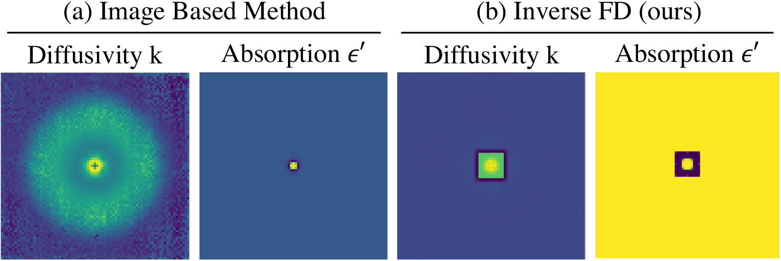
As discussed in Section 2.3, one of the other methods to solve for k and $\epsilon^{\prime}$ is to do data-based curve fitting. So we need to solve for k and $\epsilon^{\prime}$ given a set of linear equations, where we would know the values of $u_{t}$ and the Laplacian term $\Delta u_{x,y,z}$. Ideally once we have $u_{C}(x,y,z,t)$, the time derivative and Laplacian can be calculated using finite difference approximation. The drawback here is that we do not have $u_{C}(x,y,z,t)$ for all values of $z$ but only for $z=0$. This means from the image based values $u_{C}(x,y,z=0,t)$, we can get $u_{t}$ and only the $x$ and $y$ terms of the Laplacian $\Delta u_{x,y,z}$ but not the z term $u_{zz}$. So if we do the data-based curve fitting on this surface data, we will be ignoring the $u_{zz}$ term which leads to inaccurate results. Fig. 5(a, b) demonstrates the inaccuracies observed in the recovered values of diffusivity $k$ over the surface of the material.

Notice the doughnut shaped diffusivity result obtained for $k$ in Fig. 5(a). Intuitively, this is because we ignore the diffusion taking place in the depth dimension. This is one of the main reasons we shift from the data-based solution to Finite Difference (FD) Method described in Section 3.2.

Once we convert our TSF into the thermal parameters, we use those to characterize the materials and classify them into different categories and also identify them. We make 4 categories of materials - fabric, wood, paper, and metals. We have a dictionary of 22 different materials, each material falling into one of the four categories.

For known materials, we create a scatter plot using the recovered values of diffusivity $k$ and absorption parameter $\epsilon^{\prime}$ as shown in Fig. 6(b). For each material, we take multiple readings by changing its orientation and initial temperature. Our method is robust to these variations and gives clusters of data points for each of the materials. Once we have this dictionary, we can use the recovered $k$ and $\epsilon^{\prime}$ obtained from an unknown material and classify it into one of the material classes. We use a multi-layer perceptron (MLP, one hidden layer with 90 neurons) as our classifier for its simplicity and speed, and its suitability for small dataset. We train the MLP classifier on the dictionary we create and use that to classify a new material based on $k$ and $\epsilon^{\prime}$. We also experiment and compare performance with other suitable classifiers - Support Vector Classifiers (SVC, nuSVC), and Random Forest classifier (RF) (refer Table 1, Section 4.3).

We use ANSYS Fluent FEM Analysis Software for simulating the heat diffusion process. We use a custom function to define the heat injection which we allow to penetrate to a certain depth. We model this injection to be equivalent of using a relatively high power laser to heat the objects. Modeling the laser means that we also need to simulate the Gaussian beam profile of the heating source.

We can choose one of the existing materials or can create a new one based on the properties from Eq. 5 and Eq. 6b. We model the custom heat injection based on our laser source and choose its intensity accordingly. We assume same surface penetration depth for all materials (the penetration is so low that we can assume it only hits the surface layer of our discretized voxel grid). We run the simulations for 40 seconds, with the heat source being on for $t_{ON}$ = 20 seconds. We use a timestep $\Delta t$ of 0.25s. The total size of our object is 50mm $\times$ 50mm $\times$ 30mm where each discretized voxel size is $\Delta x$ = $\Delta y$ = $\Delta z$ = 0.5mm.

For the simulation process, we define a mesh on a cuboid and only take the surface readings from the simulation. A thermal camera would also provide us only surface readings, so we use these simulated surface contours as ground truth to train our FD model and test its performance. We used a material from ANSYS library (wood) with thermal properties as - density $\rho=700$ kg/$\text{m}^{3}$, specific heat $C_{p}=2310$ J/(kg K) and thermal conductivity $\sigma=0.173$ W/(m K). From Eq. 5, the thermal diffusivity of this material is $1.069\times 10^{-7}$ $\text{m}^{2}$/s. When we solve the inverse problem stated above using our FD optimization framework, we obtain a diffusivity value of $1.066\times 10^{-7}$ $\text{m}^{2}$/s, which is very close to that of the ground truth value.

Fig. 1(a) shows our experimental setup. We use a FLIR A655sc thermal camera, which has a resolution of 640 $\times$ 480, and works in the LWIR range from 7-15 $\mu$m, and a 633 nm, 60 mW laser with an Aruduino controlled relay switch. This power rating ensures that the laser is powerful enough to heat while safe enough to use. We control the system remotely as any warm body present near the setup can hamper with the readings because of thermal radiation.

We use a spatially varying source, a gaussian profiled laser beam. We use a total capture time of 60 seconds, in which the laser in on for $t_{ON}$ = 20 seconds. In the streaming mode of the camera, we capture 300 frames for 60 seconds, implying each time step measures $\Delta t$ = 0.20 seconds. We found that our approach resulted in similar results for a total capture duration of 20s or higher, detailed analysis on this is presented in the supplementary. Our algorithm can also handle multiple simultaneous scans as shown in Fig. 8(a) We placed a graded ruler in the scene next to the target objects to calibrate the physical size of each pixel. We perform this calibration every time we move the setup, but on average our value of spatial $\Delta\textbf{x}$ was 0.5 mm (same for all dimensions). This process could be automated using structured light methods (refer Section 6).

We code the differentiable FD algorithm in python using PyTorch Paszke_PyTorch_An_Imperative_2019. We use an ADAM classifier with a decreasing learning rate for 400 epochs. Our system consisting of an RTX 3060, takes 5 minutes for the process to complete and recover the $k$ and $\epsilon^{\prime}$ maps. We captured measurements for each material in different initial temperatures and orientations. The code along with the dataset has been released.

In this section, we analyze the experimental observations made in lab and look at the performance of our parameter recovery and classification algorithms.

Similar to saponaro2015material, we chose a few materials from the coarse categories of fabric, wood, paper, and metals. We made a dataset consisting of 22 materials or subclasses, applied our recovery algorithm on the data and used the generated features to train the classifier. Since metals have very low absorption and high diffusion, their TSF variation tends to have a very low magnitude. Since the $\epsilon^{\prime}$ values are almost zero for metals, the FD algorithm did not converge for them. Although we cannot differentiate between different metals, this can be used as an indicator for metals. The data in Fig. 6(a) for metals validates the theory for metals. Barring the conducting materials, we performed FD analysis on the other materials and present our analysis on them.

Fig. 6 shows a plot of $k$ vs $\epsilon^{\prime}$ sampled at the center pixels of their recovered maps. For each measurement, we generate a feature vector by sampling $k$ vs $\epsilon^{\prime}$ in a window of specified size around the center. This feature vector along with the material label forms our training set for the classification algorithm. We perform a leave-one-out cross validation approach to obtain the classification accuracy of our method. The classification results can be found in the confusion matrix in Fig. 7(b). We obtain an overall accuracy of 85.9% using a multi-layer perceptron (MLP) classifier with a feature size of 50 pixels. With more features, the subclasses become more separable compared to what we see in Fig. 6(b). We also compare performance with varying feature sizes and classifiers suitable for dataset Table 1.

Materials that have similar diffusivity, and similar absorptivity for red wavelength (used in our experiments), produce similar TSFs. This in turn makes the recovered properties of these materials similar to each other. Such an issue occurs for brown tissue and wool as seen in Fig. 6(b) and Fig. 7(b) where the algorithm gets confused between the two. This can be mitigated by using more lasers like red, green and blue which gives us a set of absorption coefficients enabling more efficient segregation.

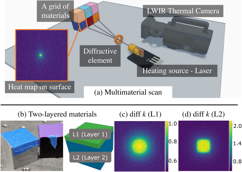
An advantage of thermal material classification over other methods like spectroscopy is that analyzing the heat diffusion can give us information that is hidden to the eye (even the thermal one). Consider a system as shown in Fig. 8(b), where the top layer is a different material from the one below it. When we inject heat, the upper layer absorbs it based on its surface and absorption properties, while the diffusion is affected by the diffusivity of both the upper layer and the layer underneath. We analyzed this problem in simulation where we assume a known thickness of upper layer but unknown thermal parameters. We used the FD forward model and optimized for diffusivity values - for the surface as well as the underneath layer, and the absorption coefficient of the surface layer. Fig. 8(c,d) show the recovered thermal properties for our simulations. We assumed a thickness of 0.5 mm and obtained the diffusivity values of the two layers with 0.01% error. This shows promise in the approach and is a good direction for future work.

References

- (1) Patitapabana Parida, Ajit Behera, and S Chandra Mishra. Classification of biomaterials used in medicine. International Journal of Advances in Applied Sciences (IJAAS), 2012.
- (2) Joerg Hendrix. Technologies for the identification, separation and recycling of automotive plastics. Int. J. Environmentally Conscious Design & Manufacturing, 5(1):35–47, 1996.
- (3) Alfons Buekens and Xujian Zhou. Recycling plastics from automotive shredder residues: A review. Journal of Material Cycles and Waste Management, 16(3):398–414, 2014.
- (4) Oliver Wang, Prabath Gunawardane, Steve Scher, and James Davis. Material classification using brdf slices. In 2009 IEEE Conference on Computer Vision and Pattern Recognition, pages 2805–2811. IEEE, 2009.
- (5) Neda Salamati, Clément Fredembach, and Sabine Süsstrunk. Material classification using color and nir images. In Color and Imaging Conference, volume 2009, pages 216–222. Society for Imaging Science and Technology, 2009.
- (6) Kenichiro Tanaka, Yasuhiro Mukaigawa, Takuya Funatomi, Hiroyuki Kubo, Yasuyuki Matsushita, and Yasushi Yagi. Material classification using frequency-and depth-dependent time-of-flight distortion. In Proceedings of the IEEE Conference on Computer Vision and Pattern Recognition, pages 79–88, 2017.
- (7) Abdelhameed F Ibrahim, Shoji Tominaga, and Takahiko Horiuchi. Spectral imaging method for material classification and inspection of printed circuit boards. Optical Engineering, 49(5):057201, 2010.
- (8) Vishwanath Saragadam and Aswin Sankaranarayanan. Programmable spectrometry: Per-pixel material classification using learned spectral filters. IEEE Intl. Conf. Computational Photography (ICCP), 2020.
- (9) Zackory Erickson, Eliot Xing, Bharat Srirangam, Sonia Chernova, and Charles C Kemp. Multimodal material classification for robots using spectroscopy and high resolution texture imaging. In 2020 IEEE/RSJ International Conference on Intelligent Robots and Systems (IROS), pages 10452–10459. IEEE, 2020.
- (10) Philip Saponaro, Scott Sorensen, Abhishek Kolagunda, and Chandra Kambhamettu. Material classification with thermal imagery. In Proceedings of the IEEE Conference on Computer Vision and Pattern Recognition, pages 4649–4656, 2015.
- (11) Jakub Bednarek, Michal Bednarek, Piotr Kicki, and Krzysztof Walas. Robotic touch: Classification of materials for manipulation and walking. In 2019 2nd IEEE international conference on Soft Robotics (RoboSoft), pages 527–533. IEEE, 2019.
- (12) Jun Zhang, Han Li, Aiguo Song, Yizhuang Ding, and Juan Wu. Thermal perception for information transmission: Theoretical analysis, device design, and experimental verification. IEEE Transactions on Haptics, 2022.
- (13) Mohamed Guiatni, Abdelaziz Benallegue, and Abderrahmane Kheddar. Thermal display for telepresence based on neural identification and heat flux control. Presence: Teleoperators and Virtual Environments, 18(2):156–169, 2009.
- (14) Anshul Singhal. Development of thermal displays for haptic interfaces. PhD thesis, Massachusetts Institute of Technology, 2016.
- (15) Amine Tilioua, Laurent Libessart, and Stéphane Lassue. Characterization of the thermal properties of fibrous insulation materials made from recycled textile fibers for building applications: Theoretical and experimental analyses. Applied Thermal Engineering, 142:56–67, 2018.
- (16) WJ Parker, RJ Jenkins, CP Butler, and GL Abbott. Flash method of determining thermal diffusivity, heat capacity, and thermal conductivity. Journal of applied physics, 32(9):1679–1684, 1961.
- (17) Robert D Cowan. Pulse method of measuring thermal diffusivity at high temperatures. Journal of Applied Physics, 34(4):926–927, 1963.
- (18) I Garrido, S Lagüela, R Otero, and P Arias. Thermographic methodologies used in infrastructure inspection: A review—post-processing procedures. Applied Energy, 266:114857, 2020.
- (19) Theodore L Bergman, Adrienne S Lavine, Frank P Incropera, and David P DeWitt. Introduction to heat transfer. John Wiley & Sons, 2011.
- (20) Richard Haberman. Applied partial differential equations, volume 4. Prentice Hall Upper Saddle River, NJ:, 2003.
- (21) Qi Guo, Emma Alexander, and Todd Zickler. Focal track: Depth and accommodation with oscillating lens deformation. In Proceedings of the IEEE international conference on computer vision, pages 966–974, 2017.
- (22) Emma Alexander, Qi Guo, Sanjeev Koppal, Steven Gortler, and Todd Zickler. Focal flow: Measuring distance and velocity with defocus and differential motion. In European conference on computer vision, pages 667–682. Springer, 2016.
- (23) Keith W Morton and David Francis Mayers. Numerical solution of partial differential equations: an introduction. Cambridge university press, 2005.
- (24) Adam Paszke, Sam Gross, Francisco Massa, Adam Lerer, James Bradbury, Gregory Chanan, Trevor Killeen, Zeming Lin, Natalia Gimelshein, Luca Antiga, Alban Desmaison, Andreas Kopf, Edward Yang, Zachary DeVito, Martin Raison, Alykhan Tejani, Sasank Chilamkurthy, Benoit Steiner, Lu Fang, Junjie Bai, and Soumith Chintala. PyTorch: An Imperative Style, High-Performance Deep Learning Library. In H. Wallach, H. Larochelle, A. Beygelzimer, F. d’Alché Buc, E. Fox, and R. Garnett, editors, Advances in Neural Information Processing Systems 32, pages 8024–8035. Curran Associates, Inc., 2019.
- (25) Martin Landmann, Stefan Heist, Anika Brahm, Simon Schindwolf, Peter Kühmstedt, and Gunther Notni. 3d shape measurement by thermal fringe projection: optimization of infrared (ir) projection parameters. In Dimensional Optical Metrology and Inspection for Practical Applications VII, volume 10667, pages 9–18. SPIE, 2018.
- (26) Martin Landmann, Stefan Heist, Patrick Dietrich, Henri Speck, Peter Kühmstedt, Andreas Tünnermann, and Gunther Notni. 3d shape measurement of objects with uncooperative surface by projection of aperiodic thermal patterns in simulation and experiment. Optical Engineering, 59(9):094107, 2020.
- (27) Jack Erdozain, Kazuto Ichimaru, Tomohiro Maeda, Hiroshi Kawasaki, Ramesh Raskar, and Achuta Kadambi. 3d imaging for thermal cameras using structured light. In 2020 IEEE International Conference on Image Processing (ICIP), pages 2795–2799. IEEE, 2020.
- (28) Maziar Raissi, Paris Perdikaris, and George E Karniadakis. Physics-informed neural networks: A deep learning framework for solving forward and inverse problems involving nonlinear partial differential equations. Journal of Computational physics, 378:686–707, 2019.
- (29) Shengze Cai, Zhicheng Wang, Sifan Wang, Paris Perdikaris, and George Em Karniadakis. Physics-informed neural networks for heat transfer problems. Journal of Heat Transfer, 143(6), 2021.
- (30) Zhili He, Futao Ni, Weiguo Wang, and Jian Zhang. A physics-informed deep learning method for solving direct and inverse heat conduction problems of materials. Materials Today Communications, 28:102719, 2021.