Unitarity and Vilenkin’s wave functions
Abstract
It is remarkably difficult to reconcile unitarity and Vilenkin’s wave function. For example, the natural conserved inner product found in quantum unimodular gravity applies to the Hartle-Hawking wave function, but fails for its Vilenkin counterpart. We diagnose this failure from different angles (Laplace transform instead of Fourier transform, non-Hermiticity of the Hamiltonian, etc) to conclude that ultimately it stems from allowing the connection to become imaginary in a section of its contour. In turn this is the unavoidable consequence of representing the Euclidean theory as an imaginary image within a fundamentally Lorentzian theory. It is nonetheless possible to change the underlying theory and replace the connection’s foray into the imaginary axis by an actual signature change (with the connection, action and Hamiltonian remaining real). The structural obstacles to unitarity are then removed, but special care must still be taken, because the Euclidean theory a priori has boundaries, so that appropriate boundary conditions are required for unitarity. Reflecting boundary conditions would reinstate a Hartle-Hawking-like solution in the Lorentzian regime. To exclude an incoming wave in the Lorentzian domain one must allow a semi-infinite tower of spheres in the Euclidean region, wave packets travelling through successive spheres for half an eternity in unimodular time. Such “Sisyphus” boundary condition no longer even vaguely resembles Vilenkin’s original proposal.
I Introduction
The fate of unitarity in the deep quantum gravity/cosmology regime is a matter of debate. Preserving unitarity may be seen as a challenge to be faced by any successful quantum gravity theory LeeReview; it may also be a mirage: an approximate concept valid only in the semi-classical limit, to be abandoned as soon as we plunge into the Planck epoch Vil-interpretation. Without wanting to take sides on this dispute, in this paper we investigate the practicalities of implementing unitarity in the context of Vilenkin’s proposal for the wave function of the Universe vil-PRD; Vil-review.
We base our efforts on recent work HHpackets showing how unimodular gravity unimod1; unimod; UnimodLee1; alan; daughton; sorkin1; sorkin2 may be used to improve the physical interpretation of the Hartle-Hawking proposal Hartle and Hawking 1983 and its compliance with unitarity. In the formulation of unimod, the unimodular gravity extension demotes the cosmological constant from a pre-given parameter to a classical constant of motion, with a conjugate momentum providing a physical measure of time: unimodular time unimod; Bombelli; UnimodLee2. Quantum mechanically, this permits superpositions of Hartle-Hawking wave functions with different to form wave packets UnimodLee2; Hartle and Hawking 1983. This suggests an inner product, with respect to which these packets and other physical states are normalizable. More importantly, the evolution in unimodular time is unitary with respect to this inner product. In view of this conservation, it is possible to set up a probability interpretation valid beyond the semi-classical limit.
None of this applies to Vilenkin’s “tunneling” wave function vil-PRD; Vil-review, which seems at odds with any implementation of unitarity and probability, a feature which appears to be intentional Vil-interpretation. In this paper we re-examine the tunneling wave function, first from the point of view of the connection, rather than the metric representation (Section II), then from the additional perspective of the unimodular extension (Sections III and IV). A number of promising first results are found in Section II by translating the monochromatic (fixed ) solutions from metric to connection representation. However, any attempts to lift the procedure in HHpackets (reviewed in Section III) to the Vilenkin setup fail. We are thus unable to provide an equivalent definition of probability. We diagnose this failure from different angles. In Section IV we note that Vilenkin’s proposal requires the connection to stray off the real line CSHHV, leading to the unavoidable use of the Laplace transform instead of the Fourier transform. The inverse Laplace transform then places the probability on the Hartle-Hawking contour only. In Section V we blame something more fundamental: the non-Hermiticity of the Hamiltonian.
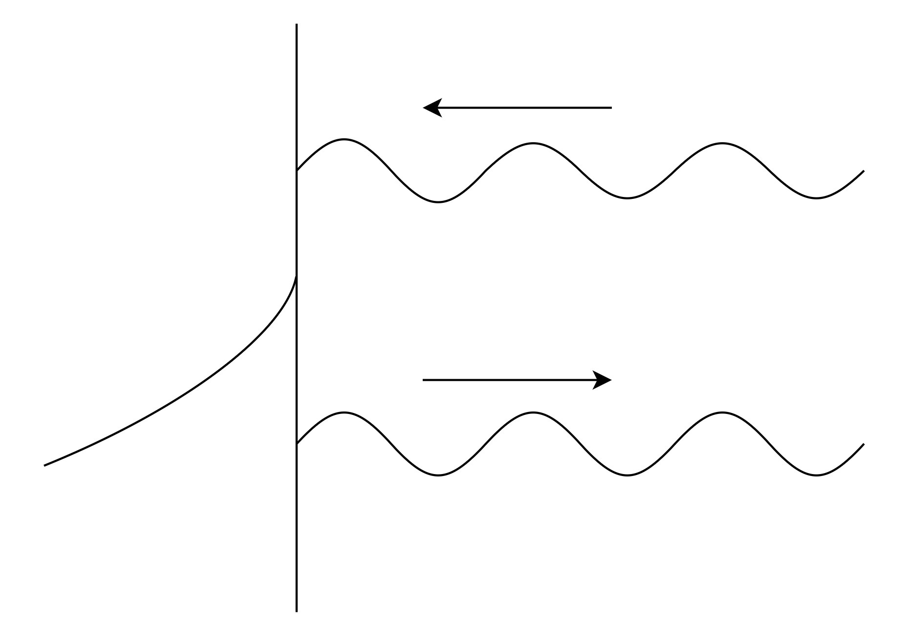
This failure is physically intuitive. The Hartle-Hawking and Vilenkin proposals loosely correspond to the two situations depicted in Fig. 1. In metric space the Hartle-Hawking wave function (left) can be seen as the reflection of an incident wave off a wall, resulting in a reflected wave and an evanescent wave penetrating the classically forbidden region. The Vilenkin wave function (right) amounts to an evanescent wave spitting out an outgoing wave, with the conspicuous absence of an incident wave. This is hardly an acceptable physical situation under our standard intuition on conservation of probability. But quantum gravity is not standard, and two new ingredients arise from the use of the connection representation instead of the metric representation, and the use of unimodular time to resolve a problem (the problem of time) not usually found in standard quantum mechanics. In Sections IV and V, however, we show that these additions do not qualitatively change anything.
Mathematically, however, there is hope. Both our diagnoses stem from allowing the connection to become imaginary in part of its domain CSHHV. This is the unavoidable consequence of representing the Euclidean theory as an imaginary image within a fundamentally Lorentzian theory (Section VI). But what if the Universe undergoes a signature change as part of the action, so that the classical trajectories themselves follow a path from the Euclidean sphere to the Lorentzian de Sitter space time (Section VII)? This is totally different from the instanton obtained by allowing the connection to go over the imaginary domain. With this assumption, the connection, action and Hamiltonian remain real, so that the structural obstacles to unitarity are removed.
However, as described in Section VIII, we still have work to do because the theory has boundaries (a 4-sphere is finite). In order to obtain an outgoing without incoming wave we must discount a reflection at the South pole and indeed continue the Euclidean half sphere with an infinite tower of spheres, playing the role of the proverbial turtles in ancient cosmologies (Sections IX and X). This continuation does not rely on a theory of gravity allowing degenerate metrics, and so a classical gluing of the North pole of one sphere with the South pole of the one above. The wave function never peaks at the gluing point (as our central Fig 6 illustrates). As unimodular time progresses a superposition of peaks at non-singular points in adjoining spheres is found, with a gradual handover between the two.
This phenomenon is reminiscent of the singularity resolution described in GielenSing, and it may help stave off runaway perturbation instabilities at North/South joining points, as described in Refs. JL1; JL2; JL3; Witten; JeanLuc, specifically JeanLuc (but see also Vilreply1; Vilreply2). Indeed this possibility can be seen as a major motivation for our work. If the fixed- monochromatic background is deemed unphysical from the unimodular perspective, one might not be too surprised that the fluctuations around it are unbounded. The construction of physical packets could open up the doors to a solution to these instabilities from the unimodular perspective. The fact that we have to modify the original Vilenkin proposal so much before this can be implemented shows how problematic the proposal is. It remains to be seen whether the fact that the Universe is never semiclassical at the problematic points is sufficient to resolve the problem.
 |
 |
II First hopes
The first ingredient in this paper is the use of the connection representation, rather than the more frequently used metric representation. Except for very standard situations, the choice of representation in the quantum theory is not innocuous. It can lead to inequivalent theories: for example with different natural inner products and probability interpretations. It may also shed new light on boundary conditions. The reason why the position representation is usually favoured in standard Quantum Mechanics is that it is physically clearer for defining boundary conditions. In Quantum Gravity it is far from obvious which representation should receive primacy in this respect. The first hope in this paper is to reassess the chasm between the Hartle-Hawking and Vilenkin’s choices from the point of view of the connection representation.
At first sight, the dictionary between metric and connection representations is straightforward CSHHV. Recall that the action can be written as:
| (1) |
where is the expansion factor, is the only minisuperspace connection variable (an off-shell version of the Hubble parameter, since on-shell, if there is no torsion), is the spatial curvature, is the lapse function and is the comoving volume of the region under study, assumed finite throughout this paper (in the quantum cosmology classical literature one usually chooses and ; see Afshordi for a discussion of the criteria for the choice of ). Throughout this paper we will assume and (we do not set since the comoving volume is left as an open scale).
Upon quantization this action implies the complementarity relation:
| (2) |
so that the wave functions in the 2 representations are just Fourier duals:
| (3) |
This is vindicated by the concrete solutions. The connection space solution is the Chern-Simons-Kodama state:
| (4) |
Inserting in (3) we find the integral representation of the Airy functions making up the Hartle-Hawking and Vilenkin wave functions, with the proviso that the choice of contour in space determines whether Hartle-Hawking (real line) or V (positive real line and negative imaginary line) is obtained (see CSHHV for details).
But is there more to it? What if we reassessed the issue of boundary conditions and probability interpretation starting from the connection representation? In the metric representation there is a physical picture of the Universe tunnelling “out of nothing”. In this language the “nothing” is the point , so what is its counterpart in the connection representation? The Hamiltonian constraint:
| (5) |
implies that classically is equivalent to (with , as will be assumed throughout this paper). These points are absent from the contour leading to the Hartle-Hawking wave function (the real line), but one of them:
| (6) |
lies on the contour leading to the V wave function (specifically the negative imaginary axis). What is so special about this point for the Chern-Simons wave function?
At this point it is easy to be beguiled by an interesting coincidence. In the metric representation, the probability of tunneling out of is is obtained via a Klein-Gordon current interpretation of probability vil-PRD; Vil-review, and when applied to the V wave function gives:
| (7) |
(we have adapted the standard result to our conventions, as in Albertini). But we could also take the Chern-Simons-Kodama state, plot along the contour leading to the V wave function to find that this is flat in along the the positive real , but not in the imaginary section of the contour. Indeed has a maximum at , tailing off along the negative imaginary axis towards on one side, and connecting with the plateau along the positive real line (the classical region) on the other side (see Fig.2). Computing the ratio between the classical plateau and this maximum we get:
| (8) |
i.e. precisely (7) (numerical factor of 12 included). This is a remarkable coincidence, strongly pointing to a reinterpretation of the standard metric/KG current result from the alternative connection point of view.
Unfortunately, none of this is left standing upon closer mathematical scrutiny. First of all, what right to we have to compute probabilities with Born’s prescription? How does this tally with unitarity?11 1 The “coincidence” highlighted in this Section is related to the fact that even in the metric representation the Klein-Gordon result can also be obtained by a basic ratio of Born factors: see Eq.(3.17) in Vil-review.
III Unitarity and the Unimodular extension
At this point it is useful to review recent progress on the issue of time, normalizability and unitarity in the context of the Hartle-Hawking wave function. As shown in HHpackets, by extending the theory to unimodular gravity, we can obtain both a physical time variable and a natural inner product, to enforce unitarity.
III.1 The unimodular extension
We use the Henneaux and Teitelboim formulation of “unimodular” gravity unimod, where one adds to a “base action” (e.g. standard General Relativity) a new term:
| (9) |
where for later convenience we have used:
| (10) |
(the “frequency” appearing in the Chern-Simons-Kodama state). Here is a density, so that the new term is diffeomorphism invariant without the need of a factor in the volume element or of the connection in the covariant derivative. Since the metric and connection do not appear in the new term, the Einstein equations and other standard field equations are left unchanged. The only new equations of motion are:
| (11) | |||||
| (12) |
i.e. on-shell-only constancy for (the defining characteristic of unimodular theories unimod1; unimod; alan; daughton; sorkin1; sorkin2) and the fact that is proportional to a prime candidate for relational time: 4-volume time unimod; unimod1; UnimodLee1; Bombelli; UnimodLee2. Reduction to minisuperspace leads therefore to:
| (13) |
where is given by (1) and we identify ). Classically nothing changes except that ’s constancy appears as an equation of motion, and the conjugate of satisfies:
| (14) |
III.2 Quantum unimodular theory
However, the quantum mechanics is very different, since:
| (15) |
Hence, we can choose either the (i.e. ) representation, leading to the standard Wheeler-DeWitt equation with solution (4), or the dual time representation, leading to (see sign0; sign; CSunimod):
| (16) |
that is, Schrodinger equation:
| (17) |
with:
| (18) |
From the unimodular point of view, the Chern-Simons-Kodama state (4) is just the spatial (in the sense of non-time) factor, , of a monochromatic wave, with the general solution being the superposition:
| (19) | |||||
where the linearizing variable for the waves sign:
| (20) |
is the Chern-Simons functional. Such wave packets can then be translated into the metric representation HHpackets via (3). For Hartle-Hawking packets (real ) we can also find the general solution by writing (17) as:
| (21) |
with solutions
| (22) |
explaining why is called the linearizing variable (it removes the dispersive nature of the medium).
What follows applies strictly to the Hartle-Hawking wave function sign; CSunimod. Then, (and so ) are real and cover the whole real line. This suggests the natural inner product involving the amplitudes:
| (23) |
Given the Fourier form in the variable of the superpositions (19), we can use the inverse Fourier transform to find:
| (24) |
assuming that and vary without any constraints on the real line (this is to be seen as the boundary condition, or lack thereof, for the imposition of unitarity). This FT is not to be confused with (3) relating metric and connection representations. This is the advantage of using the connection representation: instead of Airy functions, the are plane waves in the Chern-Simons functional.
We can therefore identify an equivalent inner product to (23) in the connection representation. Either by using (24) or by invoking Parseval’s theorem, Eq. (23) is equivalent to:
| (25) |
which is time-independent (since it is equal to (23) where does not feature), so that unitarity has been enforced. Hence the probability in term of is:
| (26) |
where we stress a measure factor multiplying the Born : the derivative of the Chern-Simons functional (and so the corresponding terms in the Hamiltonian constraint).
IV Failure of the unimodular approach in Vilenkin’s case
Regrettably, this approach—applicable to the Hartle-Hawking wave function—is lost in translation into the V wave function. This happens because has an imaginary section CSHHV in order to reproduce the V wave function, and therefore so does the Chern-Simons functional . Thus, the assumptions for using the FT break down.
We could take the view that Hartle-Hawking and Vilenkin are analytical continuations of each other (something pointed out at least as far back as in vil-PRD), so that we should replace the FT transform by the complex Laplace transform to accommodate the V wave function. The unimodular extension then still leads to the superpositions (19) seen as the Laplace transform:
| (27) |
with real and complex , after identifications:
| (28) |
(up to conventional factors of ). What follows applies both for leading to the bilateral Laplace transform, or for , leading to the standard Laplace transform22 2 It may seem that this makes a difference for convergence. Usually is a Gaussian centered on a positive : this has a tiny support in . However, for the V contour it would make the wave packets divergent as . As, it happens, the problems are more serious, and restricting makes no difference..
The problem appears in the inversion formula (24) and consequent use of Parseval’s theorem (both of which have versions for either the standard or the bilateral Laplace transform). The inversion formula is:
| (29) |
where is a real number so that the contour is in the region of convergence of . We can always choose so that the contour is the Hartle-Hawking contour. Consequently Parseval’s theorem, leading to the probability interpretation, reads:
The relevant integrations leading to the amplitudes and the probability density only care about the wave function along the Hartle-Hawking contour.
This is a damning conclusion. If we see Hartle-Hawking and Vilenkin as analytically related, and apply the unimodular prescription to define a conserved inner product, we find that the inner product expressed in terms of the connection ignores the analytical extension leading to V, and refers us back to the Hartle-Hawking theory as if no analytical extension had been made.
V The nail in the coffin
This is unsurprising. In Section III we derived unitarity directly from the fact that the inner product is defined via Eq. (23) in terms of -independent amplitudes. We then derived the equivalent expression (25), in terms of the time-dependent wave functions, which must therefore also be independent. The usual way to prove unitarity, via the Hermiticity of the Hamiltonian, can therefore be bypassed, but nonetheless it sheds light on why the argument in Section III fails for the Vilenkin contour.
Indeed we could have integrated (17) via the evolution operator (with respect to ):
| (30) |
The conservation of is enforced by , i.e. the unitarity of (and hence the terminology). This is guaranteed by the Hermiticity of () which is straightforward to prove under inner product (25), assuming is unbounded and real.
For the Hartle-Hawking wave function this is a very roundabout way to prove the time-independence of an inner product which is true by construction; but it shows why the equivalent construction for the Vilenkin wave function (allowing for a imaginary and ) cannot work. The problem is fundamentally that is anti-Hermitian if is imaginary.
Another way to see how this comes about concerns the last identity in (18), arising from:
| (31) |
implying that the Hamiltonian with inner product (25) is anti-Hermitian whenever is imaginary. This should not be confused with the fact that is not Hermitian even for the Hartle-Hawking contour, where is real. Note that implies:
| (32) |
but for real (Hermitian) the fact that is non-Hermitian does not conflict with this because:
| (33) |
However, if has non-real eingenvalues then it also cannot be Hermitian. Where is imaginary, the first term in is , instead of , creating the real problem.
Finally, we note that there are other trivial constructions for Hartle-Hawking that do not carry over to the Vilenkin setting. For example, for real and we can write the solutions to (21) as . This lies behind the conservation of probability with measure (the wave functions are non-dispersive in ). If is not real this argument collapses.
VI Euclidean image in Lorentzian theory
Had we started from an Euclidean signature (with all quantities taking real values), only the sign of the kinetic term, , in action (1) would be modified:
| (34) |
This can be worked out from first principles, but is often inferred from an analytical extension of the Lorentzian theory. Writing:
| (35) |
with fixed lapse function (or equivalently with coordinate fixed)33 3 The sign ambiguity is a source of great controversy, but it will play no role in what follows. we find that the Lorentzian action (1) becomes:
| (36) |
with and:
| (37) |
Comparing with (34) we see that the imaginary Lorentzian action is related to their the Euclidean counterpart by:
| (38) |
We can also consider an Euclidean version of the unimodular extension mimicking:
| (39) | |||||
| (40) |
so Euclidean unimodular time can be seen as imaginary Lorentzian time and vice versa. Finally, we can define an Euclidean version of the Chern-Simons functional:
| (41) | |||||
| (42) |
Within a Lorentzian theory allowing the connection to become imaginary is equivalent to an Euclidean theory with a real connection ; however the Lorentzian action is now imaginary. Therefore, the Vilenkin contour implies that the action is of the form:
| (43) |
The excursion of into the imaginary domain can be seen as an Euclidean image within the Lorentzian theory, that is, keeping the fundamental action as , so that the action is imaginary in the relevant domain. This is the origin of all the problems with unitarity.
Wherever the action is imaginary, the Hamiltonian is imaginary. The Poisson brackets are also imaginary, so that:
| (44) | |||||
| (45) |
for the Hermitian and . Upon quantization with these rules the Hamiltonian therefore is anti-Hermitian, just as we found in Section V. The wave functions in connection space, along the imaginary section of the connection, are real and evanescent. Unitarity is lost.
The conflict between unitarity and the Vilenkin proposal is therefore deeply ingrained in the structure of the theory and it is hard to see how it can be bypassed.
VII Euclidean action and signature change
In the above it is easy to forget that the Euclidean theory exists in its own right, with a real action and connection, without reference to the Lorentzian theory. We could have associated the Vilenkin contour with a different theory, in which there is an actual signature change at , from Lorentzian to Euclidean, the connection remaining real. Instead of (43) the action then is:
| (46) |
that is, the perennially real action:
| (47) |
where
| (48) |
The commutators are now imaginary and the Hamiltonian is Hermitian, as they should be. Since the action is always real, there is no need to complexify the time variable in the unimodular extension in the Euclidean section:
| (49) |
Unimodular time remains real throughout.
The Hamiltonian constraint and EOM for this theory are:
| (50) | |||||
| (51) | |||||
| (52) | |||||
| (53) |
Since the change in happens at no new term appears in (51). The usual consistency relations obtained from dotting the Hamitonian constraint and comparing with the EOM are satisfied, i.e. there is no conflict with the Bianchi identities.
The classical solutions are a conflation of the Lorentzian and Euclidean solutions. For we have:
| (54) | |||||
| (55) |
and for :
| (56) | |||||
| (57) |
corresponding to the iconic half deSitter glued to half a 4-sphere, except that this now is a classical solution. The Chern-Simons functional of this theory is always imaginary (so the wave functions are never evanescent; they propagate even in the Euclidean phase, as we shall see), that is is always real with:
| (58) |
matching (42) for . The unimodular time is also real and given by:
| (59) |
It is easy to find its on-shell expressions. For example for we have
| (60) | |||||
where we have adjusted the integration constant in so that marks the transition from Euclidean to Lorentzian signature. The solutions satisfy:
| (61) |
throughout. No issues should therefore arise with unitarity on the grounds highlighted in the previous Section. Conserved (non-dispersive in ) travelling waves can be expected in the quantum theory.
However we note a novelty. The point is now the endpoint of the manifold, or the no-boundary South Pole. Hence the Chern-Simons functional and unimodular time are limited from below by:
| (62) |
marking the beginning of the Universe. Far from being a no-boundary, unimodular time has a boundary. Therefore, we are still not off the hook regarding unitarity, since we have a theory with a boundary. We now proceed to make this problem explicit and solve it.
VIII The Euclidean quantum theory
Let us first study unitarity in an Euclidean theory with real action (rather than its imaginary image as seen from the Lorentzian theory). Since the theory’s variables and Hamiltonian are real, a priori there should be no problems quantizing it to obtain a unitary theory. Eq. (46) with implies:
| (63) | |||||
| (64) |
(where ), and quantization proceeds as:
| (65) |
where
| (66) |
is the (real) Chern-Simons functional adapted to Euclidean signature. We therefore recover Schrödinger equation (17) with a which is Hermitian with inner product (25) if and are allowed unrestricted variation. There are no obstructions to rewriting this as (21) with this , with solutions . It is straightforward to see that if and are unrestricted, the methods in HHpackets for enforcing unitarity follow through.
However, unrestricted variation in and in this context is problematic. The catch is in that the Euclidean Chern-Simons function (66) upon which wave functions depend (and providing the inner product measure) is non-monotonic, so that the inverse is multi-valued if we do not restrict to (see Fig.3). The projection of the norm (25) onto is ill-defined if no restrictions are applied.
We should therefore restrict the domain as:
| (67) |
and so:
| (68) |
This makes sense from the point of view of the classical theory, since the classical solution is a 4 sphere, which can be parameterized by (56) and (57), implying . However, the quantum theory does not a priori need to mimic the classical solution: the wave function could be an evanescent wave outside . But as we have seen, the reason for excluding this is that would then be multivalued, rendering undefined.
Imposing this restriction leaves us in territory familiar to the literature using the metric formalism GielenMenendez: if variables are restricted, then the Hamiltonian is Hermitian only if suitable boundary conditions are imposed. The standard argument applied to our setup reads:
| (69) | |||||
i.e. the integration by parts generates two boundary terms which require more onerous boundary conditions than the simple fall off conditions for when the limits lie at infinity.
Discounting non-local boundary conditions (e.g. , transferring the wave function non-locally from North to South pole of the same sphere), the obvious solution is reflecting boundary conditions:
| (70) |
(where is real and unrestricted). However this creates a number of technical problems (as we explain briefly in Section X). Also, it has the implication of reflecting the wave back into the Lorentzian domain. We then find a contracting and an expanding Universe in the Lorentzian region, in contradiction with Vilenkin’s proposal, where only an expanding travelling wave should be present.
IX Sisyphus boundary conditions
One alternative, leading to an outgoing but no incoming wave in the Lorentzian region, is a semi-infinite tower of Euclidean spheres. To Hawking’s rhetorical question, “what is south of the South pole?”, one can retort (as did Tom1; Tom2): “another North pole”. This “south of nowhere” process can be continued ad (semi) aeternum, from South of the sphere to North of the sphere; indeed this is required should we insist on unitarity together with an outgoing without incoming wave in the Lorentzian region. A reflection at any South pole down the tower of spheres would only increase the interval in unimodular time between the incoming and outgoing waves in the Lorentzian region44 4 Also, to be pedantic, going backwards in unimodular time, any reflection on a North pole after a reflection off a South pole would only send the wave down the tower, ultimately visiting the semi-infinite tower of spheres..
An infinite tower of spheres is already in use as a mathematical device for implementing reflecting boundary conditions for a single sphere via an “images” method (as we will review in Section X). In that context only the sphere exists, but one avails oneself of infinite copies with identifications:
to obtain the wave function satisfying the boundary conditions, as it bounces back and forth between North and South poles. In contrast, we posit that the spheres are distinct, with each South pole glued to the North pole below:
Such solutions exist classically within the Einstein-Cartan formalism or any formalism allowing for degenerate metrics Horowitz; Tom1, but as we will comment later, our construction is more general.
In such a setting, in the Euclidean region the wave function satisfies Schrödinger’s equation (17), that is, (21) with:
| (71) |
where , and indexes the various spheres. This then connects with the Lorentzian (valid for ) at and (see Fig. 5). Crucially
| (72) |
since the South pole of the sphere and North pole of the sphere have the same .
The range of is now the whole real line, and with suitable fall-off conditions at infinity we have unitarity with inner product (25) just as for the Hartle-Hawking wave function (see Section III). The wave functions are generic functions of the form , such that:
| (73) |
but in the Euclidean region the wave functions have support only in . By construction the normalization is time independent. We can still ask what happens in the argument leading to the “boundary” terms in (69) as we jump from the North to the South of the next sphere, but this amounts to reading off from (72) that:
| (74) |
so the boundary terms from contiguous spheres cancel out. Note that because of the determinant measure the probability density at any N or S is zero:
| (75) |
This is very interesting, as it points to an unconventional transition between spheres as we now show.
Let us consider semiclassical states by choosing a Gaussian centered on and with a spread . This leads to wave packets sign; Hartle and Hawking 1983:
| (76) |
with . The classical solution is depicted in Fig.4 and combines (54) and (55) in the Lorentzian region with a repetition of (56) and (57) (restricted so that is enforced55 5 See the discussion in the next Section for what happens if we allow .) in the Euclidean region. For as long as the wave packets remain sharply (and single) peaked, they follow and, as we have seen, this is equivalent to the classical trajectory.
The semi-classical approximation, however, badly breaks down near the transitions from one sphere to the next. This is illustrated in Fig. 6. What happens there is reminiscent of the singularity resolution in a radiation dominated Universe proposed in GielenSing. Here (as in GielenSing) the probability is always zero at the degenerate gluing point between spheres (at the classical singularity, in GielenSing). As the classical trajectory approaches a North pole, we must therefore deviate from the semi-classical limit, since the peak of the probability cannot go there. What happens is that the probability peak stops its motion at a fixed distance to the North pole, dependent on . As Fig. 6 shows, a symmetric peak then appears, equally distant from the South pole of the next sphere up the tower. As unimodular time progresses, the second peak grows at the expense of the first one. At the time when the classical trajectory would have reached the degenerate point, the wave function is actually a perfectly balanced superposition between these two peaks at non-degenerate points (middle panels of Fig. 6). As time progresses the new peak comes to dominate and the old one is suppressed. As evolves by more than , the peak starts to move along the new sphere, from South to North pole, following the classical trajectory, until a new transition starts.
The fact that the N/S degenerate point is never reached seems to imply that this construction is more general than classical theories allowing for degenerate metrics. The transition between spheres may be seen as a truly quantum phenomenon.
Note that strictly speaking the action in this setting should be
| (77) |
instead of (46), since the counter appears in phase space. Another alternative is to use:
| (78) |
but this falls within the remit of another set of theories currently being investigated.
X Are there other options?
Within unimodular theory that does not seem to be the case. The obvious alternative, reflecting boundary conditions within a single sphere, presents a number of problems. One could use an “images method” for reflections off infinitely tall potential walls for implementing the boundary conditions in that case interfreflex. Recall that for a single infinite wall (crossing out , say) one would take a normalized solution of the free unrestricted Schrodinger equation and construct for . This enforces the reflecting boundary condition, and is normalized in , in spite of the interference terms. Adapting this to two infinite walls we could get solutions for the single Euclidean sphere (or half a sphere glued to a Lorentzian manifold).
However, this would require accepting a theory with classical solutions , that is with waves traveling in both directions, in contradiction with the first order equation (21). This is possible, but it would require extending the theory to accept . The solutions (56) and (57) can then be extended to accept expansion factor (in analogy with the cosmological representation of a patch of AdS), and waves in and moving in two directions. A series of images can thus be built, describing the wave function being reflected back and forth between North and South pole (or just once off the South pole, if required).
Two major flaws can be found. First, as already stated, the wave function would be reflected back to the Lorentzian domain, generating Hartle-Hawking packets, i.e. requiring both an expanding and a contracting Universe. One could consider several reflections, with the Lorentzian branches both in the of the theory, or with one in the , but certainly we would not recover the Vilenkin asymptotic requirement. Second it is not clear that such a theory would be unitary. The inner product would have to be modified to accommodate solutions traveling in both directions. Perhaps with an entirely different construction this would be possible: namely a theory with a first order current.

Given that we would gain nothing from this complication (i.e. we would be back to Hartle-Hawking Lorentzian conditions), we will not explore this possibility further in this paper. But note that the the fact that we have a reflection within the same sphere is physically different from having multiple distinct spheres. The former leads to interference between reflected and incident waves (revealing the internal beats of packets in the probability) near the reflecting pole and a Hartle-Hawking packet in the Lorentzian region; the latter has no interference and we can indeed have only outgoing packets.
XI Conclusions
In this paper we have tried and failed to implement unitarity for the Vilenkin wave function in the unimodular extension of gravity. The failure resides squarely in the connection’s detour into the imaginary domain, associated with the Vilenkin boundary condition. This is true for the monochromatic partial waves (with fixed ) and contaminates the construction of wave packets in unimodular theory. The usual setup for a conserved inner product (so successful for packets of Hartle-Hawking wave functions) then fails. Attempts to use the Laplace transform in lieu of the Fourier integral only force the probability to live on the Hartle-Hawking connection contour. More structurally, the problem is that imaginary connections lead to anti-Hermitian Hamiltonians and so anti-unitarity. This is the unavoidable consequence of seeing the Euclidean theory (wherein the “nothing” lies) as a complex image within a Lorentzian theory. Time, connection and Chern-Simons functional then necessarily become imaginary, and unitarity is lost.
Without prejudice to the work of HHpackets (where none of these complications are found for the Hartle-Hawking state) or the stated intentions of Vil-interpretation (to regard unitarity as a mere approximation subject to breaking down), in this paper we put forward an alternative. The connection detour into the imaginary domain, usually seen as an Euclidean image within a Lorentzian theory, could also be interpreted as an actual transition from Euclidean to Lorentzian signature within a fundamentally real theory. If that is the case, all variables, action and Hamiltonian remain real, so that no structural obstacles to unitarity are found.
Nonetheless, the question still arises as to what happens at the boundary (the South pole) of the (now real) half-sphere. We proposed that a way to enforce unitarity whilst keeping a single (outgoing) wave in the Lorentzian domain is to allow the wave function to travel through a tower of spheres for an eternity in unimodular time. Such solutions do exist in gravity formulations allowing for degenerate metrics, but we stress that we could envisage our proposal as a purely quantum construction, required by unitarity and Vilenkin asymptotics. We found that semiclassical solutions with a peak following the classical equations become essentially quantum at the degenerate gluing points. Hence our proposal could even apply to standard GR, but only quantum mechanically.
We may call this proposal “Sisyphus boundary conditions”, since it is a time-reversal of Sisyphus’ ordeal. Sysiphus was condemned to roll a ball uphill only for it roll down restarting the cycle for the whole of a future eternity. In our proposal the wave function climbs up and down an infinite tower of distinct spheres for a past eternity. In the same way that Sisyphus’ punishment avoids death, ours avoids birth, i.e. a moment of cosmic creation. Ultimately this is the reason why unitarity is kept, whilst complying with Vilenkin’s boundary conditions in the Lorentzian region.
We close with a few comments on the relation between our proposal and work found in the literature. One objection to a tower of spheres is that should one try to put a general quantum field theory on this background, then the action cannot be made to converge, due to the gluing points Witten; JeanLuc (more generally one has to face the instabilities unveiled in JL1; JL2; JL3). But as we saw, the degenerate points are never reached by the peak of the wave function, with the evolution at transition unimodular times being intrinsically quantum. So the concept of quantum fields on top of a classical background breaks down at these points. In addition the evaluation of the path integral for the background assumes that the metric (and presumably the connection) is complexified to bypass such points, something that does not happen here. Another objection targets the whole concept of semi-classical time in the first place, as suggested in notime. Are these two facts sufficient to allay the concerns of JL1; JL2; JL3; Witten; JeanLuc? A translation between canonical and the path integral approach is non-trivial, and what is meant by ”contour”, ”measure”, ”convergence”, etc is strictly speaking not the same. For this reason it is hard to see what the implications are, for example, for the concept of “fuzzy instantons” (e.g. fuzzy). A full evaluation of this issue from the path integral point of view is left to future work.
We finally stress that our proposal is fundamentally different from postulating a cyclic Chern-Simons functional, , and so a cyclic unimodular time, . We could consider a cyclic unimodular time, , related to our by:
| (79) |
with and . The fact that our is built from a cyclic process plus a integer counter, , should not be seen as an anomaly. Every practical clock is the result of a periodic process (the oscillation of a pendulum, the vibration of a crystal, etc) plus a counter. Our timing system (in years, weeks, etc) also “wraps” around, triggering a counter. Since our time is not imaginary, there is no good reason to make it cyclic.
XII Acknowledgments
We thank Steffen Gielen, Jean-Luc Lehners and Alex Vilenkin for discussions related to this paper. This work was supported by FCT Grant No. 2021.05694.BD (B.A.) and the STFC Consolidated Grant ST/T000791/1 (J.M.).
References
- (1) L. Smolin, doi:10.1142/9789812702340_0078 [arXiv:hep-th/0408048 [hep-th]].
- (2) A. Vilenkin, Phys. Rev. D 39 (1989), 1116 doi:10.1103/PhysRevD.39.1116.
- (3) A. Vilenkin, “Quantum cosmology and the initial state of the Universe,” Phys. Rev. D 37 (1988), 888–897.
- (4) A. Vilenkin, Phys. Rev. D 50 (1994), 2581-2594 doi:10.1103/PhysRevD.50.2581 [arXiv:gr-qc/9403010 [gr-qc]].
- (5) B. Alexandre and J. Magueijo, Phys. Rev. D 107, no.6, 063501 (2023) doi:10.1103/PhysRevD.107.063501; [arXiv:2210.02179 [hep-th]].
- (6) W. G. Unruh, Phys. Rev. D40, 1048 (1989); K. V. Kuchař, “Does an unspecified cosmological constant solve the problem of time in quantum gravity?,” Phys. Rev. D 43 (1991), 3332–3344.
- (7) M. Henneaux and C. Teitelboim, “The cosmological constant and general covariance,” Phys. Lett. B 222 (1989), 195–199.
- (8) L. Smolin, “Quantization of unimodular gravity and the cosmological constant problems,” Phys. Rev. D 80 (2009), 084003, arXive: 0904.4841.
- (9) A. Daughton, J. Louko, and R. D. Sorkin, “Instantons and unitarity in quantum cosmology with fixed four-volume,” Phys. Rev. D 58, 084008 (1998).
- (10) A. Daughton, J. Louko, and R. D. Sorkin, “Initial conditions and unitarity in unimodular quantum cosmology,” [gr-qc/9305016].
- (11) R. D. Sorkin, “Role of time in the sum-over-histories framework for gravity,” Int J Theor Phys 33, 523–534 (1994). https://doi.org/10.1007/BF00670514
- (12) R. D. Sorkin, “Forks in the road, on the way to quantum gravity,” Int J Theor Phys 36, 2759–2781 (1997). https://doi.org/10.1007/BF02435709
- Hartle and Hawking (1983) J. B. Hartle and S. W. Hawking, “Wave Function of the Universe,” Phys. Rev. D 28 (1983), 2960–2975.
- (14) L. Bombelli, W. E. Couch and R. J. Torrence, Phys. Rev. D 44, 2589-2592 (1991) doi:10.1103/PhysRevD.44.2589
- (15) L. Smolin, Phys. Rev. D 84, 044047 (2011) doi:10.1103/PhysRevD.84.044047 [arXiv:1008.1759 [hep-th]].
- (16) J. Magueijo, “Equivalence of the Chern-Simons state and the Hartle-Hawking and Vilenkin wave-functions,” Phys. Rev. D 102 (2020), 044034.
- (17) S. Gielen and J. Magueijo, EPL 141, no.5, 59001 (2023) doi:10.1209/0295-5075/acbc48 [arXiv:2204.01771 [hep-th]].
- (18) J. Feldbrugge, J. L. Lehners and N. Turok, Phys. Rev. Lett. 119 (2017) no.17, 171301 doi:10.1103/PhysRevLett.119.171301 [arXiv:1705.00192 [hep-th]].
- (19) J. Feldbrugge, J. L. Lehners and N. Turok, Universe 4, no.10, 100 (2018) doi:10.3390/universe4100100 [arXiv:1805.01609 [hep-th]].
- (20) A. Di Tucci and J. L. Lehners, Phys. Rev. D 98, no.10, 103506 (2018) doi:10.1103/PhysRevD.98.103506 [arXiv:1806.07134 [gr-qc]].
- (21) E. Witten, “A Note On Complex Spacetime Metrics,” [arXiv:2111.06514 [hep-th]].
- (22) C. Jonas, J. L. Lehners and J. Quintin, JHEP 08, 284 (2022) doi:10.1007/JHEP08(2022)284 [arXiv:2205.15332 [hep-th]].
- (23) A. Vilenkin and M. Yamada, Phys. Rev. D 98, no.6, 066003 (2018) doi:10.1103/PhysRevD.98.066003 [arXiv:1808.02032 [gr-qc]].
- (24) A. Vilenkin and M. Yamada, Phys. Rev. D 99, no.6, 066010 (2019) doi:10.1103/PhysRevD.99.066010 [arXiv:1812.08084 [gr-qc]].
- (25) N. Afshordi and J. Magueijo, Phys. Rev. D 106, no.12, 123518 (2022) doi:10.1103/PhysRevD.106.123518 [arXiv:2209.07914 [hep-th]].
- (26) E. Albertini, S. Alexander, G. Herczeg and J. Magueijo, JCAP 11, 036 (2022) doi:10.1088/1475-7516/2022/11/036 [arXiv:2203.12640 [gr-qc]].
- (27) S. Yamashita, Phys. Rev. D 104, no.8, 086029 (2021) doi:10.1103/PhysRevD.104.086029 [arXiv:2110.13762 [gr-qc]].
- (28) J. Magueijo, Phys. Lett. B 820, 136487 (2021) doi:10.1016/j.physletb.2021.136487 [arXiv:2104.11529 [gr-qc]].
- (29) J. Magueijo, Phys. Rev. D 106, no.8, 084021 (2022) doi:10.1103/PhysRevD.106.084021 [arXiv:2110.05920 [gr-qc]].
- (30) S. Gielen and L. Menéndez-Pidal, “Singularity resolution depends on the clock,” Class. Quant. Grav. 37 (2020), 205018, arXive 2005.05357; S. Gielen and L. Menéndez-Pidal, “Unitarity, clock dependence and quantum recollapse in quantum cosmology,” arXive 2109.02660.
- (31) H. F. Westman and T. G. Zlosnik, Annals Phys. 361 (2015), 330-376 doi:10.1016/j.aop.2015.06.013 [arXiv:1411.1679 [gr-qc]].
- (32) J. Magueijo, M. Rodríguez-Vázquez, H. Westman and T. Złośnik, Phys. Rev. D 89 (2014) no.6, 063542 doi:10.1103/PhysRevD.89.063542 [arXiv:1311.4481 [gr-qc]].
- (33) G. T. Horowitz, Class. Quant. Grav. 8, 587-602 (1991) doi:10.1088/0264-9381/8/4/007
- (34) R. W. Robinett, Quantum Mechanics: Classical Results, Modern Systems, and Visualised Examples (Oxford University Press, 2006); M. Andrews, American Journal of Physics 66, 252 (1998); https://doi.org/10.1119/1.18854
- (35) J. Magueijo and L. Smolin, Universe 5, 84 (2019) doi:10.3390/universe5030084 [arXiv:1807.01520 [gr-qc]].
- (36) D. h. Yeom, Universe 7 (2021) no.10, 367 doi:10.3390/universe7100367 [arXiv:2106.10790 [gr-qc]].