Tensor Recovery in High-Dimensional Ising Models

The $k$-tensor Ising model (see [5, 43, 26, 12, 41]) is a probability distribution on the set $\{-1,1\}^{p}$, defined as:

where $\bm{J}:=((J_{r_{1},\ldots,r_{k}}))_{(r_{1},\ldots,r_{k})\in[p]^{k}}$ denotes a $k$-fold tensor with $[p]:=\{1,\ldots,p\}$ and

Hereafter, we will assume that the tensor $\bm{J}$ satisfies the following properties:

1. (1)

   $\bm{J}$ is symmetric, i.e., $J_{r_{1},...,r_{k}}=J_{r_{\sigma(1)},...,r_{\sigma(k)}}$ for every $(r_{1},\ldots,r_{k})\in[p]^{k}$ and every permutation $\sigma$ of $\{1,...,k\}$,

2. (2)

   $\bm{J}$ has zeros on the diagonals, i.e., $\bm{J}_{r_{1}...r_{k}}=0$, if $r_{s}=r_{t}$ for some $1\leqslant s<t\leqslant k$.

We will also assume that $p\geq 4$ and $2\leq k\leq p-1$ for technical reasons that will become clear later. Suppose that we are given a collection $\mathfrak{X}^{n}:=$ $\left\{\bm{x}^{(1)},\ldots,\bm{x}^{(n)}\right\}$ of $n$ samples from the model (1). Our aim is to infer the underlying tensor $\bm{J}$ based on this sample $\mathfrak{X}^{n}$. A common example of such a tensor $\bm{J}$ is the adjacency of a $k$-uniform hypergraph. Analogous to the principal goal of graphical model selection, a natural aim in this setup is to recover the hyperedge set of the tensor $\bm{J}$. In this article, we consider the slightly stronger problem of signed hyperedge recovery. To elaborate, we define the signed-edge tensor corresponding to $\bm{J}$ as:

where $\mathrm{sgn}(t):=t/|t|$ (if $t\neq 0$) and $\mathrm{sgn}(0):=0$. Following the idea in [44], we apply an $\ell_{1}$-penalized LASSO approach to recover the signed-edge tensor $\bm{J}^{*}$. Our theoretical results focus on showing consistency of the signed hyperedge recovery algorithm, for which we go beyond the classical statistical framework of fixed $p$ and $n\rightarrow\infty$, and work under a high-dimensional setting, where both $p$ and $k$ are allowed to grow with $n$. Moreover, if we define:

then we also allow the maximum degree $d$ to grow with $n$ in our framework. The precise relations between these four quantities $n,p,k$ and $d$ in order to guarantee consistent recovery of $\bm{J}^{*}$ are specified in the theoretical results in Section 2.

Recovering the signed-edge tensor $\bm{J}^{*}$ is equivalent to recovering for each vertex $r$, the vector:

where $T_{r}:=\{(r_{1},\ldots,r_{k-1})\in([p]\setminus\{r\})^{k-1}:1\leq r_{1}<\ldots<r_{k-1}\leq p\}$. For this, we implement the following node-wise $\ell_{1}$-regularized pseudolikelihood approach:

where

and $\bm{x}_{\setminus r}^{(i)}:=(x_{t}^{(i)})_{t\neq r}$. A straightforward computation shows that:

where $m_{r}(\bm{x}):=\sum_{(r_{1},\ldots,r_{k-1})\in[p]^{k-1}}J_{r,r_{1},\ldots,r_{k-1}}x_{r_{1}}\ldots x_{r_{k-1}}$.

We define the hyperedge set as $E:=\{\bm{e}\subseteq[p]:J_{\bm{e}}\neq 0\}$ and the neighborhood and signed neighborhood of each vertex $r$ respectively as:

Note that $\mathcal{N}^{\pm}(r)$ can be recovered for every vertex $r$ if we can infer the vector $\bm{J}_{r}^{*}$, for which we solve the optimization program (2).

We require certain assumptions to ensure that our method works consistently. To state these assumptions, we need a few preliminary notations. For any fixed node $r\in V$, we define a $\binom{p-1}{k-1}\times\binom{p-1}{k-1}$ matrix of the form:

which can be written more explicitly as:

where

and the $\binom{p-1}{k-1}$ dimensional vector $\bm{X}_{\cdot r}$ is defined as

When the node $r$ is clear from the context and there is no scope of any confusion, we will henceforth abbreviate $\bm{Q}_{r}$ by $\bm{Q}$. Besides, we will denote the set of all hyperedges containing $r$ by $S_{r}$ (also abbreviated by $S$ when there is no scope of confusion), i.e.

Following this notation we define $\bm{Q}_{S_{r}S_{r}}$ as the $d_{r}\times d_{r}$ sub-matrix of $\bm{Q}$ indexed by $S_{r}$. With the above notations, we are now ready to state our assumptions.

The first condition in (4) bounds the minimum eigenvalue of the Fisher information matrix corresponding to the subset of relevant covariates, and the second condition in (4) states that the relevant covariates are not overly dependent.

Condition (5) restraints the influence of the irrelevant covariates on all the relevant covariates.

The rest of the paper is organized as follows. In Section 2, we state the main theoretical results in this paper, on consistent tensor recovery, and give a brief sketch of the proof. Section 3 is devoted to applications of the recovery algorithm on some experimental and real-life neurobiological datasets. The simulation framework includes two different scenarios, one where samples are generated from Ising models on regular hypergraphs, and in another, where data is simulated from a 3-tensor Ising model on a user friendship network obtained from the Last.fm dataset. In the real-life data analysis section, the method is applied on a neurobiological dataset consisting of electro-physiological recordings from the visual cortex region in the mouse brain. The proofs of the main results are given in Section 4. In Section 5, we summarize our main contributions, and provide directions for future research. Proofs of some technical lemmas are given in the appendix.

The proof adopts the techniques in [44], modulo some modifications taking care of the tensor case. To begin with, note that the optimization problem (2) can be re-written as:

where

and $\widehat{\mu}_{r,r_{1},\ldots,r_{k-1}}:=\frac{1}{n}\sum\limits_{i=1}^{n}x^{(i)}_{r}x^{(i)}_{r_{1}}\cdots x^{(i)}_{r_{k-1}}$ are the empirical moments. The proof uses a primal-dual witness approach. The first step is to show that any optimal primal solution to (8) must vanish on all index tuples which are not hyperedges, and under standard assumptions, a unique optimal solution $\hat{\bm{J}}_{r}$ is guaranteed. The next step is to provide an upper bound to the term $\|\nabla^{2}\ell(\bm{J}_{r},\mathfrak{X}^{n})(\hat{\bm{J}}_{r}-\bm{J}_{r})\|_{\infty}$, and a lower bound on the minimum eigenvalue of $\nabla^{2}\ell(\bm{J}_{SS},\mathfrak{X}^{n})$. These together, will establish consistency of $\hat{\bm{J}}_{r}$ towards $\bm{J}$. Further details are provided in Section 4.

In this section, we present some numerical experiments that illustrate the performance of the tensor recovery algorithm. In these examples, we study the recovery rate of the algorithm based on samples simulated from Ising models on sparse hypergraphs. The built-in lib-linear solver in python “sklearn” package was used to solve the $\ell_{1}$-regularized logistic regression in all cases.

We implement our methods on neural data acquired through electrophysiological recordings from the Visual Coding Neuropixels dataset of the Allen Brain Observatory [24]. We limit our study to a male mouse aged 116 days (Session ID 791319847) with 555 neurons whose spike trains were recorded simultaneously via six Neuropixel probes. The spike trains were recorded at a frequency of 1 KHz throughout the entirety of the experiment. Our analysis focuses on the following four stimulus categories (see Figure 5) [11].

1. (1)

   Natural scenes, consisting of 118 images from three databases presented briefly for 250ms each, repeated 50 times in random order with intermittent blank intervals.

2. (2)

   Static gratings, consisting of full-field sinusoidal gratings with varying orientations, spatial frequencies, and phases, resulting in 120 conditions. Each condition is presented briefly (250 ms) before being replaced with a different condition, repeated 50 times in random order with intermittent blank intervals.

3. (3)

   Gabor patches with 3 orientations presented at different points in a 9 $\times$ 9 visual field, each presented for 250ms and repeated 50 times in random order with intermittent blank intervals.

4. (4)

   Full-field flashes, lasting for 250ms followed by a blank interval of 1.75s and repeated 150 times.

These stimuli range from natural scenes to artificial stimuli, and the purpose of this study is to explore how different stimuli patterns affect multi-neuron interactions. Dynamic stimuli such as natural movies and drifting gratings are excluded from the analysis as they require further investigation and interpretation in future studies.

To preprocess the data, we converted the spike trains, which were recorded at a frequency of 1 KHz, to a bin size of 10 ms. We achieved this by aggregating and separating them based on the start and end times of each stimulus presentation, resulting in Peri-Stimulus Time Histograms (PSTH) with a bin size of 10 ms. To obtain a smoothed version of the PSTH for each neuron and each stimulus presentation, we used a Gaussian smoothing kernel with a bandwidth of 16ms. For each stimulus presentation, we used the smoothed PSTHs as input to infer the functional connectivity (FC) between the neurons. We selected the set of neurons that were active in at least 25% of the bins in the PSTH for each stimulus presentation and collected the set of unique neurons across all stimuli. This resulted in 33, 27, 12 and 23 active neurons for natural scenes, static gratings, Gabor patches, and flashes, respectively, and a total of 44 unique active neurons overall. We further estimated the numerical derivatives of the PSTH for each active neuron and obtained a sequence with $+1$, if the derivative is positive, and $-1$, if the derivative is negative. We then abandoned the points where that derivative is $0$ and obtain 3784 out of 5950 recordings for natural scenes, 4226 out of 6000 recordings for static gratings, 2945 out of 3645 recordings for gabors and 94 out of 150 recordings for flashes. To reduce the dependence from the time series, we picked 1 in every 3 time points. For flashes, we took all the time points as samples.

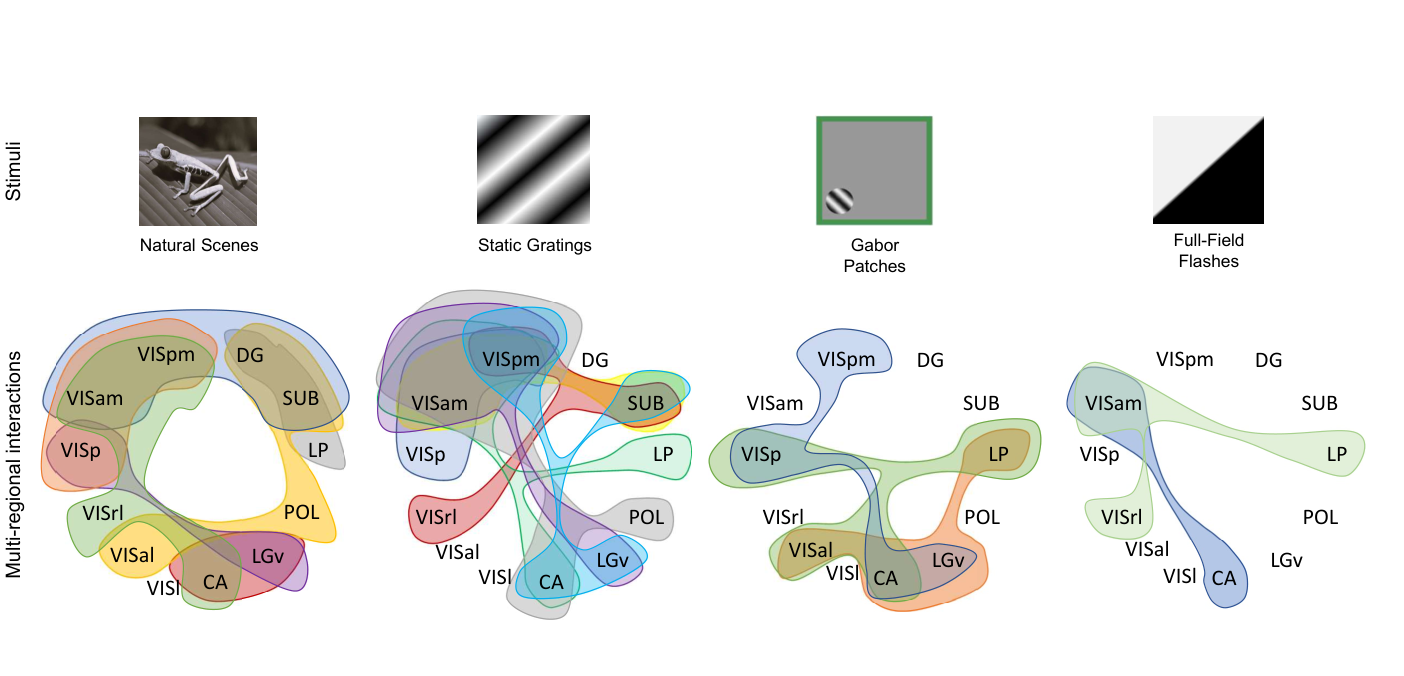
We recover the $4$-neuron interactions using a $4$-tensor Ising model, and the neuronal interactions are recovered for each stimulus type and compared across the different stimulus types. Figure 5 shows examples of such estimated multi-body interactions, after labeling the neurons based on their brain regions. For example, in the natural scenes scenario, some multi-body interactions include VISam-VISpm-DG-SUB, VISp-VISam-VISpm, VISam-VISpm-VISrl-CA, and VISal-POL-SUB-DG. In static gratings, the typical multi-body interactions noticed, are VISam-VISpm-CA-POL, VISpm-SUB-VISrl, VISam-VISpm-LGv, and VISam-VISpm-CA-POL. In Gabors, VISpm-VISp-CA-LGv, VISp-VISal-CA-LP, and VISal-CA-LGv-LP comprise some of the interactions, while in Flashes, some of these interactions include VISam-VISrl-LP and VISam-CA.

In Figure 6, we show the proportional frequencies of occurrence of different brain regions in the $4$-body interaction hyper-edges. In the natural scenes scenario, VISp has the highest frequency of occurrence, followed by SUB, VISrl, VISal, LGv, CA1 and CA3. In the static grating scenario, SUB occur with the highest frequencies, followed by LGv, CA3 and CA1. In the Gabor scenario, LGv occurs with the highest frequency, followed by VISp and VISal. Furthermore, many of the regions do not occur in any 4-body interactions, which can be explained by the fact that Gabor patches comprise of a gray screen with a small patch of gratings in a corner of the visual field of the mouse. Therefore Gabor patches is a less informative stimulus compared to natural scenes and static gratings, which can be attributed to the absence of several brain regions in the 4-body interactions. In the flashes scenario, VISam, CA3 appear with the highest frequencies, followed by VISrl and LP. Furthermore, we find that for natural scenes the regions in the visual cortex have relatively higher frequencies of occurence than the hippocampal formation and thalamus regions overall. Again, for the static gratings, the hippocampal formation have relatively higher frequency overall, compared to the other regions. In flashes, many of the brain regions do not occur in 4-body interactions, compared to the other three stimuli. This can be attributed to flashes comprising only of white or dark screen applied repeatedly to the mouse’s visual field, thereby having less information present in the visual field. Although Gabor is also a less informative stimulus overall, in contrast to flashes, Gabor comprises a patch of informative gratings restricted to a small portion of the visual field. This can lead to a few brain regions having relatively greater frequency of higher order interactions, as seen in Figure 7.

The first step of our analysis is to show the consistency of $\widehat{\bm{J}}$ under certain conditions on $(n,p,d,k,\lambda)$ and assumptions on the sample Fisher and covariance matrices:

Specifically, we assume for sometime, that Assumptions (4) and (5) hold on the sample Fisher matrix $\widehat{\bm{Q}}$ and the sample covariance matrix $\widehat{\bm{\Sigma}}$. We begin with some technical results. We start by observing that the zero subgradient condition can be written as:

with $\bm{W}:=-\nabla\ell(\bm{J};\mathfrak{X}^{n})$ for the ${\binom{p-1}{k-1}}$-dimensional score function,

It is easy to see that $\mathbb{E}_{\bm{J}}\left(\bm{W}\right)=0$. Next, applying the mean-value theorem to (14), we have:

where the remainder term is given by:

with $\bar{\bm{J}}^{(j)}$ being a parameter vector on the line segment joining $\bm{J}$ and $\hat{\bm{J}}$, and $[\cdot]_{j*}$ denoting the $j^{\mathrm{th}}$ row of the matrix. Below, we provide a probabilistic upper bound on the term $\bm{W}$.

Lemma 2 is proved in Appendix B. The following result establishes $\ell^{2}$-consistency of $\widehat{\bm{J}}_{S}$ towards $\bm{J}_{S}$.

Lemma 3 is proved in Appendix C. Finally, we control the remainder term (16).

Lemma 4 is proved in Appendix D.

To begin with, we show that Theorem 1 holds if we assume conditions (4) and (5) on the sample Fisher matrix $\widehat{\bm{Q}}$ and the sample covariance matrix $\widehat{\bm{\Sigma}}$. Moreover, this is true under the slightly weaker assumption $n>L(k!)^{8}d^{2}\log{\binom{p-1}{k-1}}$ on the sample size.

To begin with, choose $\lambda=16k![(2-\alpha)/\alpha]\sqrt{n^{-1}\log{\binom{p-1}{k-1}}}$. It then follows from Lemma 2 that with probability $1-{\binom{p-1}{k-1}}^{-1}$, we have:

Next, we verify the remaining two conditions in the hypotheses of Lemma 3 and Lemma 4. For this, note that the upper bound on $\lambda$ specified in the hypothesis of Lemma 3 is implied by the the upper bound on $\lambda$ specified in the hypothesis of Lemma 4, and hence, it is sufficient to verify the latter only. Towards this, note that:

and hence, we may choose $L>3200^{2}[(2-\alpha)/\alpha]^{4}D_{\max}^{2}/C_{\min}^{4}$, so that the hypotheses of both Lemma 3 and Lemma 4 are satisfied.

Next, let $\widehat{\bm{J}}_{S}$ be the minimizer of the partial penalized likelihood (13). Set $\widehat{\bm{z}}_{S}=\text{sign}(\widehat{\bm{J}}_{S})$ and $\widehat{\bm{J}}_{S^{c}}=0$. Then we can find a $\widehat{\bm{z}}_{S^{c}}$ that makes $\widehat{\bm{J}}$ a solution to the original convex program, thereby satisfying (15), which can be re-written in block form as:

It thus follows from (17) that:

which, on rearrangement, yields the following:

We now aim to show that $\widehat{\bm{J}}$ is a unique solution to the convex program. Towards this, note that by (18), we have:

with probability converging to one, by Lemma 4. By Lemma 1 and Assumption (4) on the sample Fisher matrix, we can thus conclude that $\widehat{\bm{J}}$ is the unique solution to the $\ell_{1}$-regularized logistic regression.

Next, we show that $\widehat{\bm{J}}_{S}$ defined by (13) satisfies $\mathrm{sgn}(\widehat{\bm{J}}_{S})=\mathrm{sgn}(\bm{J}_{S})$. In order to do so, it suffices to show that

where $J_{\min}:=\min_{\bm{e}\in E}|J_{\bm{e}}|$. From Lemma 3, we have $\|\widehat{\bm{J}}_{S}-\bm{J}_{S}\|_{2}\leqslant\frac{5}{2C_{\min}}\sqrt{d}\lambda$ so that

which is less than $1$ as long as $J_{\min}\geqslant\frac{5}{C_{\min}}\sqrt{d}\lambda$. This concludes the proof of Theorem 1 under the assumptions on the sample Fisher and sample covariance matrices.

In this section, we show that Assumptions 4 and 5 on the population Fisher and covariance matrices actually imply analogous bounds on their sample versions. This will then enable us to conclude Theorem 1 in view of Section 4.2. We start with a result guaranteeing high probability occurrence of the eigenvalue bounds (4) for the sample Fisher and covariance matrices, under the corresponding population assumptions (4).

Lemma 5 is proved in Appendix E. Now we state the analogous result for the incoherence condition (5), which guarantees sample incoherence from population incoherence.

Lemma 6 is proved in Appendix F. With Lemmas 5 and 6 in hand, we are now ready to prove Theorem 1. Towards this, define $G_{n,\delta,\alpha}:=G_{1,n,\delta}\bigcup G_{2,n,\delta}\bigcup G_{3,n,\alpha}$, where:

In view of Lemmas 5 and 6, we have:

for some constants $M,K_{1},K_{2}>0$. On the other hand, on the event $G_{n,\delta,\alpha}^{c}$, the conclusions of Section 4.2 hold. This completes the proof of Theorem 1.

References

- [1] Abeyasinghe, P. M., Aiello, M., Nichols, E. S., Cavaliere, C., Fiorenza, S., Masotta, O., … & Soddu, A. (2020). Consciousness and the dimensionality of DOC patients via the generalized ising model. Journal of Clinical Medicine, 9(5), 1342.
- [2] Agarwal, S., Branson, K. and Belongie, S. (2006), Higher order learning with graphs, Proceedings of the 23rd international conference on Machine learning, 17–24.
- [3] Anandkumar, A., Tan, V.Y.F., Huang, F, and Willsky, A.S. (2012), High-dimensional structure estimation in Ising models: Local separation criterion, The Annals of Statistics, Vol. 40 (3), 1346–1375.
- [4] Banerjee, S., Carlin, B.P., and Gelfand, A.E. (2014), Hierarchical modeling and analysis for spatial data, Chapman and Hall/CRC.
- [5] Barra, A. (2009), Notes on ferromagnetic -spin and REM, Mathematical Methods in the Applied Sciences, 32 (7): 783–797.
- [6] Barton, J., & Cocco, S. (2013). Ising models for neural activity inferred via selective cluster expansion: structural and coding properties. Journal of Statistical Mechanics: Theory and Experiment, 2013(03), P03002.
- [7] Besag, J. (1974), Spatial interaction and the statistical analysis of lattice systems, J. Roy. Stat. Soc. B, Vol. 36, 192–236.
- [8] Besag, J. (1975), Statistical analysis of non-lattice data, The Statistician, Vol. 24 (3), 179–195.
- [9] Bhattacharya, B. and Mukherjee, S. (2018), Inference in ising models, Bernoulli, Vol. 24 (1), 493–525.
- [10] Biswas, R. and Shlizerman, E. (2022), Statistical Perspective on Functional and Causal Neural Connectomics: A Comparative Study. Frontiers in Systems Neuroscience, 16:817962, https://doi.org/10.3389/fnsys.2022.817962.
- [11] Biswas, R. and Shlizerman, E. (2022), Statistical perspective on functional and causal neural connectomics: The Time-Aware PC algorithm. PLOS Computational Biology 18(11): e1010653, https://doi.org/10.1371/journal.pcbi.1010653.
- [12] Bovier, A., Kurkova, I., and Löwe, M. (2002), Fluctuations of the Free Energy in the REM and the p-Spin SK Models, The Annals of Probability, Vol. 30 (7): 605–651.
- [13] Bresler, G. (2015), Efficiently learning Ising models on arbitrary graphs, Proceedings Symposium on Theory of Computing (STOC), 771–782.
- [14] Bresler, G. (2014), Structure learning of antiferromagnetic Ising models, Advances in Neural Information Processing Systems 27 (NIPS 2014).
- [15] Bresler, G. (2020), Learning a tree-structured Ising model in order to make predictions, The Annals of Statistics, 713–737.
- [16] Cantador, I., Brusilovsky, P. and Kuflik, T. (2011), Second workshop on information heterogeneity and fusion in recommender systems, Proceedings of the 5th ACM Conference on Recommender Systems, RecSys’11, 387–388.
- [17] Cao, Y., Neykov, M. and Liu, H. (2019), High Temperature Structure Detection in Ferromagnets, arXiv:1809.08204.
- [18] Chatterjee, S. (2007), Estimation in spin glasses: A first step, The Annals of Statistics, Vol. 35 (5), 1931–1946.
- [19] Chow, C. and Liu, C. (1968), Approximating discrete probability distributions with dependence trees, IEEE Transactions on Information Theory, Vol. 14 (3), 462–467.
- [20] Comets, F. and Gidas, B. (1991), Asymptotics of maximum likelihood estimators for the Curie-Weiss model, The Annals of Statistics, 19(2):557–578.
- [21] Daskalakis, C., Dikkala, N. and Kamathm, G. (2017), Concentration of Multilinear Functions of the Ising Model with Applications to Network Data, arXiv:1710.04170.
- [22] Daskalakis, C., Dikkala, N. and Kamath, G. (2019), Testing Ising models, IEEE Transactions on Information Theory, Vol. 65 (11), 6829–6852.
- [23] Daskalakis, C., Mossel, E., and Roch, S. (2011), Evolutionary trees and the Ising model on the Bethe lattice: A proof of Steel’s conjecture, Probability Theory and Related Fields, Vol. 149 (1), 149–189.
- [24] de Vries, S. E., Lecoq, J. A., Buice, M. A., Groblewski, P. A., Ocker, G. K., Oliver, M., et. al (2020). A large-scale standardized physiological survey reveals functional organization of the mouse visual cortex, Nature neuroscience, 23(1), 138–151.
- [25] Devroye, L., Mehrabian, A. and Reddad, T. (2020), The minimax learning rates of normal and Ising undirected graphical models, Electronic J. Statist. 14 (1).
- [26] Gardner, E. (1985), Spin glasses with -spin interactions, Nuclear Physics B, 257: 747–765.
- [27] Ghosal, P. and Mukherjee, S. (2020), Joint estimation of parameters in Ising model, The Annals of Statistics, Vol. 48(2), 785–810.
- [28] Ghoshal, G., Zlatić, V., Caldarelli, G. and Newman, M. (2009), Random hypergraphs and their applications, Physical Review E, Vol. 79 (6), 066118.
- [29] Green, P.J. and Sylvia, R. (2002), Hidden markov models and disease mapping, Journal of the American Statistical Association, 97:1055–1070.
- [30] Geman, S. and Graffigne, C. (1986), Markov random field image models and their applications to computer vision, Proceedings of the International Congress of Mathematicians, 1496–1517.
- [31] Hamilton, L., Koehler, F. and Moitra, A. (2017), Information theoretic properties of Markov Random Fields, and their algorithmic applications, Advances in Neural Information Processing Systems (NIPS), 2463–2472.
- [32] Hopfield, J.J. (1982), Neural networks and physical systems with emergent collective computational abilities, Proc. Natl. Acad. Sci. USA, 79:2554–2558.
- [33] Ising, E. (1925), Beitrag zur theorie der ferromagnetismus, Zeitschrift für Physik, Vol. 31, 253–258.
- [34] Ibarrondo, R., Sanz, M. and Orús, R. (2022), Forecasting Election Polls with Spin Systems, SN COMPUT. SCI. 3, 44.
- [35] Klimm, F., Deane, C.M. and Reinert, G. (2020), Hypergraphs for predicting essential genes using multiprotein complex data, bioRxiv, https://doi.org/10.1101/2020.04.03.023937.
- [36] Lipowski, A. (2022), Ising Model: Recent Developments and Exotic Applications, Entropy (Basel). 24 (12): 1834.
- [37] Liu, Q., Huang, Y. and Metaxas, D.N. (2011), Hypergraph with sampling for image retrieval, Pattern Recognition, Vol. 44(10-11), 2255–2262.
- [38] Lokhov, A.Y., Vuffray, M., Misra, S. and Chertkov, M. (2018), Optimal structure and parameter learning of Ising models, Science Advances, Vol. 4, Issue 3.
- [39] Montanari, A. and Saberi, A. (2010), The spread of innovations in social networks, Proceedings of the National Academy of Sciences, Vol. 107 (47), 20196–20201.
- [40] Mukherjee, S. (2021), Limit Theorems for Dependent Combinatorial Data, with Applications in Statistical Inference, Publicly Accessible Penn Dissertations, 3940, https://repository.upenn.edu/edissertations/3940
- [41] Mukherjee, S., Son, J. and Bhattacharya, B. (2022), Estimation in tensor Ising models, Information and Inference: A Journal of the IMA, Vol. 11 (3), 1457–1500.
- [42] Neykov, M. and Liu, H. (2019), Property testing in high-dimensional Ising models, Annals of Statistics, Vol. 47 (5), 2472–2503.
- [43] Oliveira, V.M. and Fontanari, J.F. (1997), Landscape statistics of the -spin Ising model, Journal of Physics A: Mathematical and General, 30 (24).
- [44] Ravikumar, P., Wainwright, M. J. and Lafferty, J. D. (2010), High-dimensional Ising model selection using -regularized logistic regression, Annals of Statistics, 38 (3), 1287–1319.
- [45] Roudi, Y., Tyrcha, J., & Hertz, J. (2009). Ising model for neural data: model quality and approximate methods for extracting functional connectivity. Physical Review E, 79(5), 051915.
- [46] Santhanam, N.P., and Wainwright, M.J. (2012), Information-theoretic limits of selecting binary graphical models in high dimensions, IEEE Transactions on Information Theory, Vol. 58 (7), 4117–4134.
- [47] Tan, S., Bu, J., Chen, C., Xu, B., Wang, C. and He, X. (2011), Using rich social media information for music recommendation via hypergraph model, Vol. 7(1), Vol. 22.
- [48] Tian, Z., Hwang, T. and Kuang, R. (2009), A hypergraph-based learning algorithm for classifying gene expression and arrayCGH data with prior knowledge, Bioinformatics, Vol. 25 (21), 2831–2838.
- [49] Tkacik, G., Schneidman, E., Berry II, M. J., & Bialek, W. (2006). Ising models for networks of real neurons. arXiv preprint q-bio/0611072.
- [50] Wainwright, M. J. (2009), Sharp thresholds for high-dimensional and noisy sparsity recovery using -constrained quadratic programming (Lasso), IEEE Transactions on Information Theory, 55, 2183–2202.
Appendix A Proof of Lemma 1
Note that the penalized problem (8) can be equivalently written as a constrained optimization problem over the ball , for some constant (by Lagrange duality). The primal can be formulated as: