Optimal Transport Particle Filters
Abstract
This paper is concerned with the theoretical and computational development of a new class of nonlinear filtering algorithms called the optimal transport particle filters (OTPF). The algorithm is based on a recently introduced variational formulation of the Bayes’ rule, which aims to find the Brenier optimal transport map between the prior and the posterior distributions as the solution to a stochastic optimization problem. On the theoretical side, the existing methods for the error analysis of particle filters and stability results for optimal transport map estimation are combined to obtain uniform error bounds for the filter’s performance in terms of the optimization gap in solving the variational problem. The error analysis reveals a bias-variance trade-off that can ultimately be used to understand if/when the curse of dimensionality can be avoided in these filters. On the computational side, the proposed algorithm is evaluated on a nonlinear filtering example in comparison with the ensemble Kalman filter (EnKF) and the sequential importance resampling (SIR) particle filter.
I Introduction
Optimal transportation (OT) theory has gained significant interest recently because it provides natural geometrical and mathematical tools for analysis and manipulation of probability distributions [1, 51, 36]. In particular, two geometric notions are of key importance: (i) a metric to measure the similarity/discrepancy between probability distributions, i.e., the Wasserstein metric, and (ii) a map to transport one distribution to the other, i.e., the OT or Monge map. In contrast to their information-theoretic counterparts (such as the Kullback-Liebler (KL) divergence), these OT metrics respect the geometry of the data and are often more robust against perturbations and errors. Due to these unique features, OT metrics and maps have been successfully employed in a variety of applications, including generative modeling and sampling [4, 47], domain adaptation [11], and image processing [24, 15, 31, 21, 41].
Given the significance of OT theory, there has been a growing line of research to apply OT tools for nonlinear filtering and Bayesian inference [17, 9, 35, 46]. The central idea here is to view the filtering/Bayesian update step as the problem of transporting the prior distribution (of the current state) to the posterior distribution (of the future state). This perspective has led to the development of new algorithms for Bayesian inference, namely learning triangular transport maps with polynomial, radial basis, and neural net parameterizations to sample from posteriors [17, 28, 25], ensemble transform particle filters [34], and OT interpretations of the feedback particle filter algorithm [52, 44, 45, 46].
This paper builds on the authors’ recent work [43] where an OT-based variational formulation of the Bayes’ law was introduced to learn the OT map from the prior to the posterior distribution for any value of the observation signal. In this formulation, the conditional distribution , of a hidden random variable given the observation , is identified as , i.e., the push-forward of the prior distribution with respect to a map of the form where is a real-valued function that solves the optimization problem:
| (1) |
Here is an independent copy of and denotes the set of functions that are convex with respect to the argument for any fixed , and is the convex conjugate of with respect to the argument.
The above variational formulation enjoys three key features that distinguish it from prior works: (i) it is simulation-based in the sense that it is possible to approximate the objective function in terms of samples from the joint distribution and does not require an explicit formula for the likelihood; (ii) The variational formulation enables new approximation methods for computing the posterior distribution by choosing different subsets/parameterizations of the set ; (iii) The problem (1) is stochastic and can be solved efficiently using recent machine learning techniques, for example, can be parameterized as a deep neural network and trained using stochastic gradient descent. Problem (1) can be obtained as the dual form of a block-triangular Monge problem between the independent coupling and the joint distribution . Similar variational formulations arise in block-triangular transport of distributions in the context of conditional generative models; for example [40, 25, 32, 38, 39].
The objective of the current paper is to use the formulation (1) to develop a new nonlinear filtering algorithm, called optimal transport particle filter (OTPF), and provide preliminary theoretical analysis and numerical validation of the algorithm. The proposed algorithm can be viewed as a nonlinear and non-Gaussian generalization of the ensemble Kalman filter algorithm (EnKF) [18, 7] and the discrete-time counterpart of the feedback particle filter (FPF) algorithm [53, 52] (OTPF solves the gain function approximation and the numerical time discretization problems in the FPF altogether by solving the proposed variational problem (1)).
The theoretical analysis of the paper is concerned with the error analysis of the proposed algorithm. In particular, we study how errors solving problem (1) at each time step affect the overall performance of the filtering algorithm. To do so, we adapt the existing methods for error analysis of particle filters (PF) to obtain a uniform bound on the filtering error in terms of the approximation error of the OT map [14, 49, 8, 13]. These results are based on a strong notion of uniform geometric filter stability [6], which is common in the analysis of PF. Next, we combine this with stability results for the estimation of OT maps [22] which relates the approximation error of the map to the optimization gap of (1) (see Lemma 2) . The error analysis is carried out for the mean-field limit of the algorithm and a variant of the particle system that involves an additional resampling step which makes the particles independent of each other and significantly simplifies the analysis.
The numerical experiments qualitatively and quantitatively evaluate the performance of the OTPF in comparison with the EnKF algorithm [18, 7] and the sequential importance resampling (SIR) PF [16]. In particular, we consider a linear stable dynamical system with three different observation functions: linear, quadratic, and cubic. The numerical results illustrate the versatile nature of the OTPF compared to the other two methods.
II Problem Formulation
II-A Filtering problem
Consider a discrete-time stochastic dynamic system given by the update equations
| (2a) | ||||
| (2b) | ||||
| for where is the state of the system, is the observation, is the probability distribution for the initial state , is the probability kernel for the transition from the state to the state , and is the likelihood distribution of an observation given a state . We assume that the update equation (2a) is realized with the stochastic map | ||||
| (2c) | ||||
where is an i.i.d sequence and is Lipschitz in for all . Throughout the paper, we assume that all probability measures admit a density and use the same notation to refer to the distribution or the corresponding measure. If needed, the two notions will be distinguished depending on the context.
The filtering problem is to infer the conditional distribution of the state given the history of the observations , that is, the distribution
often referred to as the posterior distribution.
II-B Recursive update for the filter
The posterior distribution admits a recursive update equation that is essential for the design of filtering algorithms. To present this recursive update, let us introduce the following operators:
| (3a) | ||||
| (3b) | ||||
| The first operator represents the update for the distribution of the state according to the dynamic model (2a). The second operator represents Bayes’ rule that carries out the conditioning according to the observation model (2b). In terms of these two operators, the update law for the posterior is given by (e.g. see [8]): | ||||
| (3c) | ||||
where we introduced . With slight abuse of notation, we further define the transition operator as
We then have for all . Note that the transition operator is stochastic in nature as it depends on the realization of the observation signal . We suppress this dependence to simplify the presentation.
II-C Filter stability
We use the following metric on (possibly random) probability measures :
| (4) |
where the expectation is over the possible randomness of the probability measures and , and is the space of functions that are uniformly bounded by one and uniformly Lipschitz with constant smaller than one (this metric is also known as the dual bounded-Lipschitz distance). We use this metric to introduce a notion of uniform geometrical stability for the filter.
Definition 1 (Uniformly geometrically stable filter)
The filter update (3) is uniformly geometrically stable if and positive constant such that for all and it holds that
| (5) |
Remark 1
The uniform geometric stability property (5) is also used in the error analysis of PFs in [14, 13]. It can be verified if the dynamic transition kernel satisfies a minorization condition, i.e., there exists a probability measure and a constant such that . The minorization is a mixing condition that ensures geometric ergodicity of the Markov process [29]. We acknowledge that this condition is a strong and can be verified for a restricted class of systems, e.g., should belong to a compact set. A complete characterization of systems with uniform geometric stable filters is an open and challenging problem in the field. More insight is available for the weaker notion of asymptotic stability of the filter, i.e., , which holds when the system is “detectable” in a sense that is suitable for nonlinear stochastic dynamical systems [50, 10, 48, 23]. This characterization of systems with asymptotic filter stability is in agreement with the existing results for the stability of the Kalman filter, which holds when the linear system is detectable in the classical sense [30]. A complete survey of existing filter stability results can be found in [12].
The following Lemma is useful for our error analysis.
Lemma 1
Let be a (random) distribution and and two (random) measurable maps. Then,
where the expectation is over the possible randomness of the distribution as well as the maps .
Proof:
The proof follows from a straightforward argument using the definition of the metric (4) and the Lipschitz property of the test functions .
III Optimal Transport Particle Filters
The construction of OTPFs relies on the variational formulation (1). Consider the objective functional
| (6) |
where , , and is an independent copy of , along with the optimization problem
| (7) |
It is shown in [43, Prop. 1] that the solution to this problem provides an OT characterization of the Bayes operator (3b). The result is reproduced here for completeness
Proposition 1
Assume admits a density with respect to the Lebesgue measure. Then, the objective function (6) has a unique (up to a constant shift) minimizer and
| (8) |
III-A The exact mean-field process
We use the OT characterization of the conditional distribution to construct a (exact) mean-field process whose distribution is exactly equal to the posterior distribution . Consider a process with distribution defined as
| (9a) | ||||
| where is an independent copy of in the dynamic model (2c). It is then straightforward to verify that | ||||
| (9b) | ||||
where the second identitiy is a consequence of Proposition 1. It then follows that whenever then . As such, the mean-field process is called exact. The OTPF is obtained by approximating the exact mean-field process in two steps, as described next.
III-B The approximate mean-field process
The first approximation step consists of restricting the feasible set of the optimization problem (7) to a parameterized class of convex functions . The resulting approximated distribution is denoted by which follows the update rule:
| (10a) | ||||
| This update defines the approximate mean-field process | ||||
| (10b) | ||||
The approximation error between and , due to the parameterization of the function is studied in section IV-A.
III-C The finite particle system
The second approximation step is to replace the mean-field process with an empirical distribution of a collection of particles , i.e., The finite- discretization can be achieved through two different approaches leading to two different systems of particles. The first system (the particle system with resampling) is more amenable to error analysis, while the second system the interacting particle system) is more practical.
(C.I) the particle system with resampling: Define the sampling operator
| (11) |
and approximate the mean-field distribution by introducing the sampling operator within the update equations:
| (12a) | ||||
| The presence of the sampling operator ensures that the distribution is an empirical distribution formed by a collection of particles, i.e. Equation (12a) further identifies an update law for the particles: | ||||
| (12b) | ||||
where and are independent copies of . The sampling process is similar to the resampling stage in PFs, with the difference being that the weights are uniform in this case. The resampling step makes the particles independent of each other, which significantly simplifies the error analysis, as seen in Section IV-B.
(C.II) the interacting particle system: The second approach to constructing the finite- particle system is to discretize the update equation (10b) for the mean-field process according to
| (13) | ||||
The empirical distribution does not follow an update-law similar to the update law for due to the nature of the operator , which smooths out empirical distributions. Instead, the update for the interacting particle system can be expressed as
where is a stochastic operator that takes any empirical distribution and outputs . Moreover, in contrast to the previous construction (the particle system with resampling), the particles are now correlated, which makes the error analysis challenging (this is often studied under the propagation of chaos analysis [42]) We leave the error analysis of the interacting particle system as the subject of future work. However,we empirically validate the performance of this approximation in Section V.
IV Error Analysis
The objective of this section is to study the approximation error of the OTPFs introduced above. We begin with the analysis for the approximate mean-field process before turning our attention to the particle system with resampling.
IV-A The mean-field analysis
The distance between the exact mean-field distribution and the approximate distribution is characterized by the following proposition.
Proposition 2
Remark 2
The first assumption in the proposition is used to ensure the error produced at each step of the algorithm does not grow with time. The second assumption is related to the representation power of the function class relative to the class of probability distributions introduced by the algorithm . For example, this error is zero when is a class of convex and quadratic functions, and the filtering problem is based on a linear Gaussian dynamic and observation model. In this case, probability distributions are Gaussian with the corresponding quadratic optimal function . In general, it is expected that the error is small when the distributions are inherently simple, e.g. when the problem exhibits low-dimensional structures or regularities. The analysis of these errors is the subject of representation theory [3, 37]. The last assumption is related to the regularity of the distributions and the resulting posterior distributions and can be enforced by an appropriate choice of the class .
Proof:
To simplify the presentation, we introduce the operator for all , to denote the update law for the approximate mean-field distribution in (10a). The first step in the proof is to use the triangle inequality and the filter stability to bound the error between and as follows:
Next, we use Lemma 1 to bound the distance
for all . Finally, we use the second and third assumptions in the proposition to obtain a uniform bound for the error between and using Lemma 2 (is outlined below)
concluding the final bound (15).
Lemma 2
Proof:
The proof is an extension of the result [22, Prop. 10] and omitted on the account of space.
IV-B The particle-system-with-resampling analysis
Next, we analyze the error between the particle system (12) and the exact mean-field process (9). The process is similar to the mean-field analysis presented in the previous section, with an additional error due to the sampling operator and the empirical approximations.
Proposition 3
Consider the exact mean-field distribution and the particle distribution defined in (9) and (12), respectively. Assume
- 1.
The exact filter is stable according to Definition 5.
- 2.
There exists a constant such that for all and :
- 3.
For all , , and , the function is convex and is -Lipschitz.
Then, it holds that
| (16) |
where all constants are time-independent.
Proof:
The proof is similar to that of Proposition 2. Define the operator . Then, the triangle inequality and filter stability imply
Applying the triangle inequality again, we can write
By application of Lemma 1 and Lemma 2, the first term is upper-bounded by the square-root of
where we used the second and the third assumptions. This gives the first term on the right-hand side of (16). The second term is due to the sampling error and upper-bounded by since the test functions in the definition of the metric are uniformly bounded by one (e.g. see [33, Lemma 2.17]). Adding the two errors concludes the final bound.
Remark 3
The assumptions of this proposition are similar to the assumptions in Proposition 2 with a slight difference in the second assumption. The bound in the second assumption can be decomposed into two terms:
The second term is similar to the one used in Proposition 2 and related to the representation power of . The first term corresponds to the statistical generalization errors due to approximating distributions with empirical samples and the subject of statistical generalization theory [37, 5, 26, 54]. The error is expected to scale according to where the constant is a proxy for the complexity of the class of functions , and independent of the dimension . The first term can also be interpreted as the variance, while the second term is the bias. Then our error analysis is a manifestation of the bias-variance trade-off dependent on the complexity of the function class . Similar bias-variance trade-offs also appear in the analysis of local PFs in [33].
V Numerical Experiments
We use a numerical example to illustrate the proposed OTPF in comparison with two other filters: the EnKF [18], and the sequential importance resampling (SIR) PF [16].
For the OTPF, we solve a min-max formulation of the variational problem (7), as described in [43, Sec. III-B] and originally proposed in [27] for estimating OT maps. The min-max formulation involves optimization over an additional convex function which is used to represent the convex conjugate as follows:
However, in our numerical experiments, we observed that relaxing the constraint and optimizing over a map instead of produces better numerical results due to the additional freedom in the parameterization. Therefore, we use the formulation
Note that this does not change the optimization problem because the optimal is of gradient form and equal to . The final objective function takes the form
| (17) | ||||
Remark 4
Note that we changed the role of source and the target , compared to the original formulation (1), so that represents the transport map from the prior to the posterior, instead of . This formulation leads to a more convenient parameterization of the map.
Similar relaxations to the above have also been found to be beneficial for computing Wasserstein barycenters [19] and Wasserstein gradient flows [20]. Here ICNN denotes the set of partially input convex neural networks [2].
To illustrate the performance of the filters, consider the following dynamics and observation model:
| (18a) | ||||
| (18b) | ||||
for , where , and are i.i.d sequences of -dimensional standard Gaussian random variables, and . We use three observation functions:
where denotes the element-wise (i.e., Hadamard) product when is a vector.
In order to solve (17), we parameterize ICNN as
where , for , and is the size of the network. The map is modeled with a standard residual network with two blocks of size and a ReLU-activation function.
We used the ADAM optimizer to solve the min-max problem with learning rate , inner-loop iteration , and the total number of iterations , which is divided by after each time step (of the filtering problem) until it reaches . Each iteration involves a random selection of a batch of samples of size from the total of particles . Observation samples are produced using the observation model: . Samples from the independent coupling are generated by random shuffling. The number of particles is the same for all algorithms. The details of the numerical code is available online11 1 https://github.com/Mohd9485/OT-EnKF-SIR.
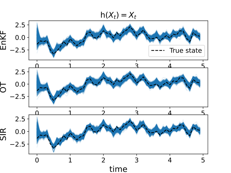
The numerical results are presented in Figure 1 for a two-dimensional problem , while the figure only shows the first component (We choose because the SIR and OT approach did not differ significantly when , while the difference became apparent with .) The figure shows the trajectory of the particles along with the trajectory of the hidden state. The first experiment, depicted in panel (a), illustrates the performance of a linear observation function. As expected, all three algorithms behave similarly as all of them are able to capture the exact solution, which is Gaussian in this case, and obtained using linear maps. The second experiment, depicted in panel (b), involves the quadratic observation function . This is an interesting case since the problem is not observable, and we expect to see a (symmetric) bimodal distribution. It is observed that EnKF fails to represent the bimodal distribution while both OT and SIR capture the two modes, although, SIR exhibits mode collapse in the time range of . Finally, both SIR and OT perform better than ENKF for the cubic observation function , depicted in panel (c), as expected due to the strong nonlinearity in the observation model.
We also quantify the performance of all algorithms in these three experiments by computing the mean-squared-error (MSE) in estimating a function of the state:
| (19) |
where the empirical average approximates the expectation over independent simulations. The results are depicted in Figure 2. For the linear and cubic observation models, we used . For the quadratic case, we used (comparing the estimated and true means is not a good criterion for the quadratic case because the distribution is bimodal with mean equals to zero).


In Figure 2-(a), it is observed that both OT and SIR filters yield results that are close to the EnKF, which is asymptotically exact for the linear case. However, in Figure 2-(b), the OT method outperforms both EnKF and SIR for the quadratic case, while the difference between OT and SIR is not significant for the cubic case, depicted in Figure 2-(c). The performance of the OT filter is expected to improve with further fine-tuning, increasing the iteration number of training, and the number of parameters in the neural net, at the cost of higher computational effort. An appropriate analysis of the efficiency of the OT method, how it scales to high-dimensional problems, and its application to more realistic data, is the subject of future work.
VI Discussion
In this paper, we presented the OTPF algorithm and provided preliminary theoretical error analysis and numerical results that demonstrated the competitive performance of our method in the presence of nonlinear observations and non-Gaussian states. We introduced several directions of future research: the verification of the geometric stability for dynamical systems e.g. of the form (18); error analysis of the optimization gap in solving the variational problem, both in terms of representation and generalization as discussed in Remark 3; error analysis of the interacting particle system without resampling; and extensive numerical experiments and comparison in truly high-dimensional settings.
References
- [1] Luigi Ambrosio, Nicola Gigli, and Giuseppe Savaré. Gradient flows: in metric spaces and in the space of probability measures. Springer Science & Business Media, 2005.
- [2] Brandon Amos, Lei Xu, and J Zico Kolter. Input convex neural networks. arXiv preprint arXiv:1609.07152, 2016.
- [3] Martin Anthony and Peter L Bartlett. Neural network learning: Theoretical foundations, volume 9. cambridge university press Cambridge, 1999.
- [4] Martin Arjovsky, Soumith Chintala, and Léon Bottou. Wasserstein generative adversarial networks. In International conference on machine learning, pages 214–223. PMLR, 2017.
- [5] Sanjeev Arora, Rong Ge, Yingyu Liang, Tengyu Ma, and Yi Zhang. Generalization and equilibrium in generative adversarial nets (gans). In International Conference on Machine Learning, pages 224–232. PMLR, 2017.
- [6] Rami Atar and Ofer Zeitouni. Exponential stability for nonlinear filtering. In Annales de l’Institut Henri Poincare (B) Probability and Statistics, volume 33, pages 697–725. Elsevier, 1997.
- [7] Edoardo Calvello, Sebastian Reich, and Andrew M Stuart. Ensemble Kalman methods: a mean field perspective. arXiv preprint arXiv:2209.11371, 2022.
- [8] Olivier Cappé, Eric Moulines, and Tobias Rydén. Inference in hidden markov models. In Proceedings of EUSFLAT Conference, pages 14–16, 2009.
- [9] Yuan Cheng and Sebastian Reich. A McKean optimal transportation perspective on Feynman-Kac formulae with application to data assimilation. arXiv preprint arXiv:1311.6300, 2013.
- [10] Pavel Chigansky, Robert Liptser, and Ramon Van Handel. Intrinsic methods in filter stability. Handbook of Nonlinear Filtering, 2009.
- [11] Nicolas Courty, Rémi Flamary, Devis Tuia, and Alain Rakotomamonjy. Optimal transport for domain adaptation. arXiv preprint arXiv:1507.00504, 2015.
- [12] Dan Crisan and Boris Rozovskii. The Oxford handbook of nonlinear filtering. Oxford University Press, 2011.
- [13] Pierre Del Moral and Pierre Del Moral. Feynman-Kac formulae. Springer, 2004.
- [14] Pierre Del Moral and Alice Guionnet. On the stability of interacting processes with applications to filtering and genetic algorithms. In Annales de l’Institut Henri Poincaré (B) Probability and Statistics, volume 37, pages 155–194. Elsevier, 2001.
- [15] Ayelet Dominitz and Allen Tannenbaum. Texture mapping via optimal mass transport. IEEE transactions on visualization and computer graphics, 16(3):419–433, 2010.
- [16] Arnaud Doucet and Adam M Johansen. A tutorial on particle filtering and smoothing: Fifteen years later. Handbook of nonlinear filtering, 12(656-704):3, 2009.
- [17] Tarek A El Moselhy and Youssef M Marzouk. Bayesian inference with optimal maps. Journal of Computational Physics, 231(23):7815–7850, 2012.
- [18] Geir Evensen. Data Assimilation: The Ensemble Kalman Filter. Springer Science & Business Media, 2006.
- [19] Jiaojiao Fan, Amirhossein Taghvaei, and Yongxin Chen. Scalable computations of Wasserstein barycenter via input convex neural networks. arXiv preprint arXiv:2007.04462, 2020.
- [20] Jiaojiao Fan, Amirhossein Taghvaei, and Yongxin Chen. Variational Wasserstein gradient flow. arXiv preprint arXiv:2112.02424, 2021.
- [21] Sira Ferradans, Nicolas Papadakis, Gabriel Peyré, and Jean-François Aujol. Regularized discrete optimal transport. SIAM Journal on Imaging Sciences, 7(3):1853–1882, 2014.
- [22] Jan-Christian Hütter and Philippe Rigollet. Minimax rates of estimation for smooth optimal transport maps. arXiv preprint arXiv:1905.05828, 2019.
- [23] Jin Won Kim and Prashant G Mehta. Duality for nonlinear filtering i: Observability. arXiv preprint arXiv:2208.06586, 2022.
- [24] Soheil Kolouri, Se Rim Park, Matthew Thorpe, Dejan Slepcev, and Gustavo K Rohde. Optimal mass transport: Signal processing and machine-learning applications. IEEE signal processing magazine, 34(4):43–59, 2017.
- [25] Nikola Kovachki, Ricardo Baptista, Bamdad Hosseini, and Youssef Marzouk. Conditional sampling with monotone GANs. arXiv preprint arXiv:2006.06755, 2020.
- [26] Shuang Liu, Olivier Bousquet, and Kamalika Chaudhuri. Approximation and convergence properties of generative adversarial learning. Advances in Neural Information Processing Systems, 30, 2017.
- [27] Ashok Makkuva, Amirhossein Taghvaei, Sewoong Oh, and Jason Lee. Optimal transport mapping via input convex neural networks. In International Conference on Machine Learning, pages 6672–6681. PMLR, 2020.
- [28] Youssef Marzouk, Tarek Moselhy, Matthew Parno, and Alessio Spantini. An introduction to sampling via measure transport. arXiv preprint arXiv:1602.05023, 2016.
- [29] Sean P Meyn and Richard L Tweedie. Markov chains and stochastic stability. Springer Science & Business Media, 2012.
- [30] Daniel Ocone and Etienne Pardoux. Asymptotic stability of the optimal filter with respect to its initial condition. SIAM Journal on Control and Optimization, 34(1):226–243, 1996.
- [31] Julien Rabin, Gabriel Peyré, Julie Delon, and Marc Bernot. Wasserstein barycenter and its application to texture mixing. In International Conference on Scale Space and Variational Methods in Computer Vision, pages 435–446. Springer, 2011.
- [32] Deep Ray, Harisankar Ramaswamy, Dhruv V Patel, and Assad A Oberai. The efficacy and generalizability of conditional GANs for posterior inference in physics-based inverse problems. arXiv preprint arXiv:2202.07773, 2022.
- [33] Patrick Rebeschini and Ramon Van Handel. Can local particle filters beat the curse of dimensionality? The Annals of Applied Probability, 25(5):2809–2866, 2015.
- [34] Sebastian Reich. A nonparametric ensemble transform method for Bayesian inference. SIAM Journal on Scientific Computing, 35(4):A2013–A2024, 2013.
- [35] Sebastian Reich. Data assimilation: The Schrödinger perspective. Acta Numerica, 28:635–711, 2019.
- [36] Filippo Santambrogio. Optimal transport for applied mathematicians. Birkäuser, NY, 55(58-63):94, 2015.
- [37] Shai Shalev-Shwartz and Shai Ben-David. Understanding machine learning: From theory to algorithms. Cambridge university press, 2014.
- [38] Yuyang Shi, Valentin De Bortoli, George Deligiannidis, and Arnaud Doucet. Conditional simulation using diffusion Schrödinger bridges. In Uncertainty in Artificial Intelligence, pages 1792–1802. PMLR, 2022.
- [39] Ali Siahkoohi, Gabrio Rizzuti, Mathias Louboutin, Philipp A Witte, and Felix J Herrmann. Preconditioned training of normalizing flows for variational inference in inverse problems. arXiv preprint arXiv:2101.03709, 2021.
- [40] Alessio Spantini, Ricardo Baptista, and Youssef Marzouk. Coupling techniques for nonlinear ensemble filtering. arXiv preprint arXiv:1907.00389, 2019.
- [41] Zhengyu Su, Yalin Wang, Rui Shi, Wei Zeng, Jian Sun, Feng Luo, and Xianfeng Gu. Optimal mass transport for shape matching and comparison. IEEE transactions on pattern analysis and machine intelligence, 37(11):2246–2259, 2015.
- [42] Alain-Sol Sznitman. Topics in propagation of chaos. Ecole d’été de probabilités de Saint-Flour XIX—1989, 1464:165–251, 1991.
- [43] Amirhossein Taghvaei and Bamdad Hosseini. An optimal transport formulation of Bayes’ law for nonlinear filtering algorithms. In 2022 IEEE 61st Conference on Decision and Control (CDC), pages 6608–6613. IEEE, 2022.
- [44] Amirhossein Taghvaei and Prashant G Mehta. An optimal transport formulation of the linear feedback particle filter. In 2016 American Control Conference (ACC), pages 3614–3619. IEEE, 2016.
- [45] Amirhossein Taghvaei and Prashant G Mehta. An optimal transport formulation of the ensemble Kalman filter. IEEE Transactions on Automatic Control, 66(7):3052–3067, 2020.
- [46] Amirhossein Taghvaei and Prashant G Mehta. Optimal transportation methods in nonlinear filtering: The feedback particle filter. arXiv preprint arXiv:2102.10712, 2021.
- [47] Ilya Tolstikhin, Olivier Bousquet, Sylvain Gelly, and Bernhard Schoelkopf. Wasserstein auto-encoders. arXiv preprint arXiv:1711.01558, 2017.
- [48] Ramon Van Handel. Observability and nonlinear filtering. Probability theory and related fields, 145:35–74, 2009.
- [49] Ramon Van Handel. Uniform observability of hidden Markov models and filter stability for unstable signals. 2009.
- [50] Ramon Van Handel. Nonlinear filtering and systems theory. In Proceedings of the 19th International Symposium on Mathematical Theory of Networks and Systems (MTNS semi-plenary paper), 2010.
- [51] Cédric Villani. Optimal Transport: Old and New, volume 338. Springer, 2009.
- [52] Tao Yang, Richard S Laugesen, Prashant G Mehta, and Sean P Meyn. Multivariable feedback particle filter. Automatica, 71:10–23, 2016.
- [53] Tao Yang, Prashant G Mehta, and Sean P Meyn. Feedback particle filter. IEEE transactions on Automatic control, 58(10):2465–2480, 2013.
- [54] Pengchuan Zhang, Qiang Liu, Dengyong Zhou, Tao Xu, and Xiaodong He. On the discrimination-generalization tradeoff in GANs. arXiv preprint arXiv:1711.02771, 2017.