Assessing stellar yields in Galaxy chemical evolution: observational stellar abundance patterns2022Assessing stellar yields in Galaxy chemical evolution: observational stellar abundance patterns–References

Jinning Liang Eda Gjergo Affiliation: School of Physics and Technology, Wuhan University, Wuhan, Hubei 430072, China Thanks: E-mail: eda.gjergo@gmail.com Affiliation: School of Physics and Technology, Wuhan University, Wuhan, Hubei 430072, China Affiliation: School of Astronomy and Space Science, Nanjing University, Nanjing 210093, People’s Republic of China Affiliation: Key Laboratory of Modern Astronomy and Astrophysics (Nanjing University), Ministry of Education, Nanjing 210093, People’s Republic of China XiLong Fan Affiliation: School of Physics and Technology, Wuhan University, Wuhan, Hubei 430072, China

Accepted XXX. Received YYY; in original form ZZZ

Abstract

One-zone Galactic Chemical Evolution (GCE) models have provided useful insights on a great wealth of average abundance patterns in many environments, especially for the Milky Way and its satellites. However, the scatter of such abundance patterns is still a challenging aspect to reproduce. The leading hypothesis is that dynamics is a likely major source of the dispersion. In this work we test another hypothesis, namely that different assumptions on yield modeling may be at play simultaneously. We compare whether the abundance patterns spanned by the models are consistent with those observed in Galactic data. First, we test the performance of recent yield tabulations, and we show which of these tabulations best fit Galactic stellar abundances. We then group the models and test if yield combinations match data scatter and standard deviation. On a fixed Milky-Way-like parametrization of NuPyCEE, we test a selection of yields for the three dominant yield sets: low-to-intermediate mass stars, massive stars, and Type Ia supernovae. We also include the production of r-process elements by neutron star mergers. We explore the statistical properties spanned by such yields. We identify the differences and commonalities among yield sets. We define criteria that estimate whether an element is in agreement with the data, or if the model overestimates or underestimates it in various redshift bins. While it is true that yields are a major source of uncertainty in GCE models, the scatter of abundances in stellar spectra cannot be explained by a simple averaging of runs across yield prescriptions.

Keywords:

galaxies: abundances – stars: abundances – Galaxy: evolution – methods: data analysis

1 Introduction

Galactic Archaeology, here used interchangeably with Galactic Chemical Evolution (GCE), works on the premise that stellar surfaces encapsulate the composition of their progenitor gas, so that little to no nucleosynthesis reaches stellar surfaces via convection or other means. While this hypothesis is simplistic for a range of stellar categories, works such as Hawkins et al. 2020 have shown that most stellar wide binary pairs have indeed an extremely homogeneous composition with a dispersion below 0.02 dex. Therefore, any composition observed in the distribution of stellar abundance patterns should reflect the past enrichment histories experienced by the progenitor gas.

GCE finds its roots in the landmark reviews by Burbidge et al. 1957, known as the B²FH paper, and by Cameron 1957, written independently. Based on the solar abundances compiled by Suess & Urey 1956, B²FH described the nucleosynthesis processes that generate a wide array isotopic species, including all the stable ones. Ever since B²FH, the field was successful in solving a number of observational challenges.

One such achievement was the Tinsley-Wallerstein diagram (Wallerstein 1962; Tinsley 1979), otherwise known as the [ $\alpha$ /Fe] vs [Fe/H] diagram. This diagram is particularly sensitive to the rates of Type Ia supernovae (SNIa), a source responsible of at least half of the iron enrichment (Matteucci et al. 2009) ahead of core collapse supernovae (SNCC), and SNCC themselves which are very effective at generating $\alpha$ species¹¹ 1 $\alpha$ species are ⁴He, ¹²C, ¹⁶O, ²⁰Ne, ²⁴Mg, ²⁸Si, ³²S, ³⁶Ar, and ⁴⁰Ca. (Matteucci 2001; Pagel 2009). Stars residing in different Galactic regions (specifically for the interests of this paper, the halo, the thick disc and the thin disc) are clustered in specific regions of the Tinsley-Wallerstein diagram, providing insights on their past history: halo stars occupy a flat [ $\alpha$ /Fe]-enhanced, [Fe/H]-poor region. The flat [ $\alpha$ /Fe] trend breaks at the age where SNIa begin to enrich the interstellar medium (ISM), [Fe/H] $\geq-1$ ²² 2 The square bracket notation represents logarithmic number densities of a species $A$ , relative to species $B$ , and normalized to solar values: $\mathrm{[A/B]}=\log\left(N_{\mathrm{A}}/N_{\mathrm{B}}\right)-\log\left(N_{\mathrm{A}}/N_{\mathrm{B}}\right)_{\odot}.$ , causing a downward [ $\alpha$ /Fe] slope toward zero (i.e., solar values) with increasing iron abundance. This region after the onset of SNIa is where thick disc stars are clustered. Lastly, thin disc stars tend to occupy a space right below thick disc stars, on a flatter [ $\alpha$ /Fe] slope.

A recent investigation of the Tinsley-Wallerstein diagram on APOGEE-DR16 data can be found in Spitoni et al. 2021, which uses MCMC methods to fit a multi-zone GCE model. The original GCE models were one-zone, meaning that the galaxy is treated as a point. In one-zone models, the metallicity and star formation rate in a galaxy are homogeneously uniform as a function of time. These type of models are still useful because of the insights they provide on the essential constituents of galaxy evolution. In fact, more sophisticated models should integrate back to the global properties that emerge from one-zone models. For a recent extensive review on GCE, refer to Matteucci 2021.

Despite the many successes and predictions of GCE models, stellar abundances are scattered across a wide range of values, and the exact origin of this scatter is not yet completely understood for every chemical element. There have been numerous attempts at reproducing these patterns, or at least at constraining the conditions that may give rise to them. Most of the models make the sensible assumption that dynamical effects are at play. Proposed phenomena include stellar migration (Schönrich & Binney 2009; Spitoni et al. 2015; Johnson et al. 2021), gas radial flow (Andrews et al. 2017; Weinberg et al. 2017; Trueman et al. 2022; Chen et al. 2022), the inclusion of a variable IMF (Yan et al. 2019) or of a stochastic star formation rate (SFR, Cescutti 2008, with a specific application to heavy elements), or Bayesian approaches (Côté et al. 2017; Rybizki et al. 2017; Spitoni et al. 2020).

In this work we explore an alternative route, namely we investigate whether multiple enrichment phenomena as described by different yield models could coexist in a Milky-Way like one-zone galaxy, and whether they may contribute to the abundance patterns of a select number of elements. We follow Romano et al. 2010, where they investigated existing yields in literature, and they evaluated which yield in each enrichment channel best fits Galactic stellar abundance data. In this work, we implement sets of more recent yields compared to Romano et al. 2010, where they already investigated Karakas 2010 and Kobayashi et al. 2006. We include also Limongi & Chieffi 2018; Nomoto et al. 2013 for massive stars, Cristallo et al. 2011; Cristallo et al. 2015 for AGBs, and Ritter et al. 2018 for both mass ranges. We overview the yield mass-fraction, final mass, initial mass, initial metallicities. We re-categorize the yields into 3 groups, according to analogous modeling motivations: hypernovae fraction, massive star initial rotational velocity, and delayed/rapid explosion prescriptions for massive stars. We then run on-zone GCE simulations with the use of the OMEGA module in NuPyCEE (Côté et al. 2017), using different yield combinations in each run. We therefore show the resulting simulated abundance ratios as a function of iron abundance. We lastly perform a statistical analysis on the aforementioned 3 groups of models and on the data at different metallicity bins. We explore trends and discrepancies.

This paper is structured as follows: Section 2 contains a description of the observed stellar abundances (Section 2.1), of the stellar yields considered in this work (Section 2.2), of the parameters chosen to run the NuPyCEE simulations (Section 2.3.1), and of the statistical criteria (Section 2.3.2) employed in the Results (Section 3). In Section 3 we also explore the performance of the models in reproducing the abundance patterns of our 12 chosen elements. Our conclusions and discussions can be found in Section 4, where the summary plots also appear.

Paper	C	N	O	Na	Mg	Al	Ca	Mn	Ni	Zn	Ba	Eu	Region of sampling
Carretta et al. 2000	$\times$	$\times$	$\times$	$\times$	$\times$								halo, thick and thin disc
Reddy et al. 2003	$\times$	$\times$	$\times$	$\times$	$\times$	$\times$	$\times$	$\times$	$\times$	$\times$	$\times$	$\times$	thin disc
Cayrel et al. 2004	$\times$	$\times$	$\times$	$\times$	$\times$	$\times$	$\times$	$\times$	$\times$	$\times$			halo
Israelian et al. 2004		$\times$	$\times$										halo
Bensby et al. 2005			$\times$	$\times$	$\times$	$\times$	$\times$		$\times$	$\times$	$\times$	$\times$	thick and thin disc
Reddy et al. 2006	$\times$		$\times$	$\times$	$\times$	$\times$	$\times$	$\times$	$\times$	$\times$	$\times$	$\times$	halo, thick and thin disc
Bensby et al. 2014			$\times$	$\times$	$\times$	$\times$	$\times$		$\times$	$\times$	$\times$		thick and thin disc
Roederer et al. 2014	$\times$	$\times$	$\times$	$\times$	$\times$	$\times$	$\times$	$\times$	$\times$	$\times$	$\times$	$\times$	halo
Zhao et al. 2016	$\times$		$\times$	$\times$	$\times$	$\times$	$\times$				$\times$	$\times$	halo, thick and thin disc
Mashonkina et al. 2017				$\times$	$\times$	$\times$	$\times$		$\times$		$\times$	$\times$	halo
Reggiani et al. 2017				$\times$	$\times$	$\times$	$\times$	$\times$	$\times$	$\times$	$\times$		halo

Table 1: Observational data, in chronological order, of the stellar elemental abundances considered in the present work. The first column indicates the references. In the subsequent 12 columns, the

\times

marks whether a paper contains that column’s element. The elements in order are C, N, O, Na, Mg, Al, Ca, Mn, Ni, Zn, Ba, and Eu. The last column indicates in which region of the Milky Way the sampled stars reside.

2 Methods

The Methods section is split among observational data, stellar yields investigated, and theoretical models. Within the theoretical models section, we include both a description of the GCE model and of the statistics criteria employed in the analysis.

2.1 Observational Data

Model	Stellar Yields		Group	Z range	M range	Comments
	LIMs	Massive stars
1	F.R.U.I.T.Y.	N13	A	[0.0001,0.05]	$\left[1.3,40.0\right]$	$f_{\mbox{HNe}}=0.5$
2	K10	K06	A	[0.0001,0.02]	$\left[1.0,40.0\right]$	$f_{\mbox{HNe}}=0.0$
3	K10	K06	A	[0.0001,0.02]	$\left[1.0,40.0\right]$	$f_{\mbox{HNe}}=0.5$
4	K10	K06	A	[0.0001,0.02]	$\left[1.0,40.0\right]$	$f_{\mbox{HNe}}=1.0$
5	K10	LC18	B	[3.236 $\times 10^{-5}$ ,0.02]	$\left[1.0,120.0\right]$	Set R, $V_{rot}=0.0$ km/s
6	K10	LC18	B	[3.236 $\times 10^{-5}$ ,0.02]	$\left[1.0,120.0\right]$	Set R, $V_{rot}=150.0$ km/s
7	K10	LC18	B	[3.236 $\times 10^{-5}$ ,0.02]	$\left[1.0,120.0\right]$	Set R, $V_{rot}=300.0$ km/s
8	K10	LC18	B	[3.236 $\times 10^{-5}$ ,0.02]	$\left[1.0,120.0\right]$	Set R, $V_{rot,avg}$
9	F.R.U.I.T.Y	NuGrid	C	[0.0001,0.02]	$\left[1.3,25.0\right]$	MESA-only (delay)
10	NuGrid	K06	A	[0.001,0.02]	$\left[1.0,40.0\right]$	$f_{\mbox{HNe}}=0.5$
11	K10	NuGrid	C	[0.0001,0.02]	$\left[1.0,25.0\right]$	MESA-only (delay)
12	NuGrid	NuGrid	C	[0.0001,0.02]	$\left[1.0,25.0\right]$	MESA-only (delay)
13	NuGrid	NuGrid	C	[0.0001,0.02]	$\left[1.0,25.0\right]$	MESA-only (delay wind pre-exp)
14	NuGrid	NuGrid	C	[0.0001,0.02]	$\left[1.0,25.0\right]$	MESA-only (mix)
15	NuGrid	NuGrid	C	[0.0001,0.02]	$\left[1.0,25.0\right]$	MESA-only (rapid)
16	NuGrid	NuGrid	C	[0.0001,0.02]	$\left[1.0,25.0\right]$	MESA-only (classical)
Index	SNIa yields			Z range		Comments
a	I99			0.02		CDD1
b	I99			0.02		CDD2
c	I99			0.02		W7
d	Ivo12			[0.0002,0.02]		Stable
e	T86			0.02

Table 2: Legend for the models (first column) adopted in the present work. Each model corresponds to a different yield variation. Numbers from 1 to 16 indicate combinations of yields coming from low-to-intermediate mass stars (LIMs) and massive stars. The indices a to e identify the Type Ia SNe (SNIa) yields paired with the above-mentioned models. The abbreviations stand for the following: NuGrid (Ritter et al. 2018); F.R.U.I.T.Y. (Cristallo et al. 2015); N13 (Nomoto et al. 2013); K06 (Kobayashi et al. 2006); K10 (Karakas 2010); LC18 (Limongi & Chieffi 2018); I99 (Iwamoto et al. 1999); Ivo12 (Seitenzahl et al. 2013); T86 (Thielemann et al. 1986). In the last column, Comments, we identify the various assumptions on the massive stellar yield computations. More details on these assumptions can be found in the text.

In this section, we summarize the observational data that appear in the present work. For our purposes, we have chosen to focus on the following elements: C, N, O, Na, Mg, Al, Ca, Mn, Ni, Zn, Ba, and Eu. The yield performance on each of these elements will be investigated in Section 3. All abundances, whether theoretical or observational, are calibrated to photospheric solar data (Asplund et al. 2009).

We consider the data-sets presented in Table 1. The last column includes the Galactic environments – namely halo, think disc, thick disc, or solar neighborhood and field stars – in which the sampled stars reside for each study. Some of these studies sampled stars residing in multiple environments:

Figure 1: Logarithmic mass-fraction (defined as the yield mass over ejecta mass) of the returned yields for 12 elements at solar metallicity, as a function of logarithmic stellar mass. The "shift" label on the upper right indicates, wherever necessary, the factor by which the mass-fractions have been shifted in order to fit the same y-axis range (e.g., the Europium mass-fraction ranges between a value of

10^{-9}

and

10^{-10}

while in the plot it ranges between

10^{-2}

and

10^{-3}

, a shift of +7 dex). The legends for different stellar yields on the first row follow the description in Table 2. The yields are styled in the following way: all of the low-to-intermediate mass stars (LIMs) yields are represented with the dash-dotted lines; the massive star yields can be represented by solid lines (Nomoto et al. 2013; Kobayashi et al. 2006), by dotted lines (Limongi & Chieffi 2018), or by dashed lines (Ritter et al. 2018). Among the LIMs yields, the colorings are: green (Cristallo et al. 2011; Cristallo et al. 2015, F.R.U.I.T.Y., ), included in Models 1 and 9; blue (Karakas 2010, K10, ) included in Models 2 to 8, and black for Model 11; pink (Ritter et al. 2018, NuGrid, ) included in Model 10, 12, 13, 15 and 16, and yellow included in Model 14.

Refer to caption — Figure 2: The ejected stellar mass versus initial stellar mass for 16 yield tables. The colorbar of the various curves represents different initial metallicities in the range of their yield tables. Here we use a logarithmic scale in the color bar. The lighter the color (yellower), the higher the initial metallicity. The blue line provides a reference, where the ejected mass equals the initial stellar mass. Groups and Models are described in Table 2.

[i]
1.

Halo stars: Cayrel et al. 2004 selected 35 high signal-to-noise ratio giants from the ESO Large Programme "First Stars", where they investigated 70 very metal-poor dwarf and giants whose spectra were captured with the ESO VLT and UVES spectrograph. 17 elemental abundances from C to Zn were reported in their work, i.e. 10 out of the 12 elements we consider. Israelian et al. 2004, on the other hand reports N and O only for 31 metal poor stars. Their spectra were measured using multiple instruments. On top of finding a scaling relation for [N/Fe] vs [Fe/H] in the range -3.1 < [Fe/H] < 0, they confirmed the necessity of a primary component to the nitrogen enrichment. Roederer et al. 2014 is one of two papers in our sample that reports abundances for all 12 elements. They report, in fact, 48 elemental abundances including an isotopic breakdown for 5 additional species for 191 of the 313 stars observed over the course of 10 years of the Magellan Inamori Kyocera Echelle campaign. Their efforts focused primarily on the [Fe/H] $\leq$ -2.5 stellar sample. Mashonkina et al. 2017 also focused on very metal-poor (-4 < [Fe/H] < -2) stars, a selection of 59 stars residing primarily in the halo, but 7 of which were found in dwarf spheroidal galaxies. We chose not to omit these stars. The traced elements are a combination of $\alpha$ - and odd-Z-elements, as well as Ni and the main neutron-capture species. They confirm their metal-poor sample is $\alpha$ -enhanced by a factor of 2 compared to solar $\alpha$ /Fe abundances. Reggiani et al. 2017 combines literature abundances with their observations to constrain GCE over a wide range of metallicities (-3.6 $\leq$ [Fe/H] $\leq$ -0.4). They find their results suggest strong inhomogeneous hypernova enrichment. Group A in our yield set includes variations on this enrichment mechanism. While they include Ba, they don’t report CNO elements or Eu.
2.

Thin disc-dominated stars: Reddy et al. 2003 is the other reference from Table 1 that investigated all the 12 elements analyzed in our work. They provide abundances for 15 additional elements for 181 F and G dwarf stars, the vast majority (Reddy et al. 2003, their Fig. 17) of which reside in the thin disc. While this work reports stellar abundances from both thin and thick disc, the prevalence of thin disc stars warrants placing them in a separate category.
3.

Thin and thick disc stars: Also Bensby & Feltzing 2006 measured chemical abundances in F and G dwarf stars, using the Coudé Echelle Spectrograph (CES), with 35 and 16 stars residing in the thin and thick disc, respectively. Similarly to Reddy et al. 2003, the thin/thick disc classification was based on kinematic criteria. The work mainly focuses on carbon trends, but measures the abundances of all of our chosen elements, with the exception of N. More recently, Bensby et al. 2014 again investigated 714 F and G disc dwarf and subgiant stars in the solar neighborhood. This work identifies the bimodality of the [ $\alpha$ /Fe]-[Fe/H] relation for thin and thick disc stars, the latter being the more $\alpha$ -enhanced, despite a significant metallicity overlap in the metal-poor to solar metallicity regime. Missing from the Bensby & Feltzing 2006; Bensby et al. 2017 papers are C, N, and Mn and, in the latter, also Eu.
4.

Halo, thick, and thin disc: On a sample of 19 extremely metal-poor stars observed with CES, Carretta et al. 2000 expanded their selection with literature data that measured high signal-to-noise (S/N > 150) spectra for 300 stars spanning a wide range of metallicities. They report abundances for light intermediate elements (C, N, O, Na, and Mg). Reddy et al. 2006 then isolated 176 solar-neighborhood F and G dwarf thick-disc candidates. While 95 stars were classified as thick disc stars, 48 could not be classified conclusively, 20 belonged to the halo while 13 to the thin disc. We therefore choose to include this paper among the halo, thick, and thin disc group. Concerning our 12 elements, Reddy et al. 2006 provides a complete set with the exception of nitrogen. Zhao et al. 2016 selects stars with the deliberate aim of collecting spectra for thin, thick disc, and halo stars from $-2.62\leq$ [Fe/H] $+0.24$ and 17 their elemental abundances from Li to Eu. Of the elements that concern our work, all are present but nitrogen and three species around the iron peak (Mn, Ni, and Zn).

2.2 Stellar Yields

In this section, we describe and compare different stellar yields. All of the yields are included in the NuPyCEE database³³ 3 https://github.com/NuGrid/NuPyCEE/tree/master/yield_tables. We define mass-fraction as the ratio of the ejected mass for a specific chemical species divided by the total ejecta mass. A comparison for different stellar yields of 12 elements at solar metallicity is also shown in Fig. 1. The yields we considered in this work and summarized in Table 1 are as follows:

[i]
1.

For low and intermediate mass stars, the yields come from: Karakas 2010; F.R.U.I.T.Y., i.e. Cristallo et al. 2011; Cristallo et al. 2015; and NuGrid, i.e. Ritter et al. 2018.
2.

For massive stars, the yields come from: Nomoto et al. 2013, Kobayashi et al. 2006, Limongi & Chieffi 2018, and (Ritter et al. 2018).
3.

For Type Ia Supernovae, the yields come from: Iwamoto et al. 1999, Thielemann et al. 1986, and Seitenzahl et al. 2013.

Most of the analysis on yield variations in our work concern massive stars. Of the four massive star yield tabulations we consider, two of them (Kobayashi et al. 2006; Nomoto et al. 2013) are by the same authors and investigate the impact to the chemical enrichment of the inclusion of hypernova yields in massive stars. Hypernova episodes are set to occur for stars in the mass range from 20 to 40 $M_{\odot}$ . The authors define the fraction of stars, $f_{HNe}$ , that will experience a hypernova episode. $f_{HNe}$ varies from 0% (Model 2) to 100% (Model 4). Three of the models (Model 1, 3, and 10 in Table 1) are set to $f_{HNe}=0.5$ . We call this yield set “Group A”.

The next set (Models 5 to 8) includes only yield variations in “Set R” – the recommended set – for Limongi & Chieffi 2018. Models 5, 6, and 7 assume that all of the massive stars rotate at rotational velocities of 0, 150, and 300 km/s, respectively. Model 8 ( $V_{rot,avg}$ ) represents an average of the 3 other rotation velocities. We call this yield set “Group B”.

Next come a series of NuGrid models computed with MESA (Paxton et al. 2015, Models 9 and 11 to 16). In the Comments column for such models, the term in the parenthesis indicates the remnant mass prescription used for the core-collapse explosion of massive stars as computed in Fryer et al. 2012. “rapid” refers to the fast-convection model, i.e. it includes explosions occurring within 0.250 s after bounce; while “delayed” refers to the delayed convection model, which also include later explosions such as the ones dominated by standing accretion shock instability. “mix” is a 50/50 mix of the delayed and rapid models, while “delay wind pre-exp” adds pre-SN nucleosynthesis and wind nucleosynthesis to the delayed model. Lastly, Model 16 is the classical approach as presented in Fryer et al. 2012. We call this yield set “Group C”.

For SNIa yields, CDD1, CDD2, W7 are the 3 different models that represent the SNIa detonation scenario from Iwamoto et al. 1999. “Stable” for Seitenzahl et al. 2013 means that the SNIa yields contain only the stable isotopes. Thielemann et al. 1986 reports only one SNIa yield set. The Type Ia SN yields are shown on the bottom of Table 1 with model indices spanning from “a” to “e”. Table 1 also reports the metallicity and mass range spanned by each yield set. Among SNIa yields, only Seitenzahl et al. 2013 reports metallicity-dependent yields in the very metal-poor vs solar-metallicity regimes.

Each of these references computes yield tabulations on different metallicity grids. The only shared metallicity is $Z=0.02$ . In Fig. 1 we show the logarithmic mass-fraction (namely the ratio of the yield expressed in solar masses vs. the ejecta mass) as a function of logarithmic masses for all 12 elements and for the various yield prescriptions. Each panel refers to a single element. Except for C, and Ba, LIMs yields have little to no dependence on the stellar mass at these near-solar metallicities. Furthermore, these models are in fairly good agreement with each other. We note that the AGB/LIMs yield paper Karakas 2010 does not contain yields for Ca, Mn, Zn, Ba, Eu.

Figure 3: Logarithmic yields versus Atomic number for the 5 SNIa yield tables, as indicated in Table 2. The atomic number range goes from 6(C) to 32(Ge)

When it comes to massive stars, there is often a clear dependence of the mass-fraction on the initial stellar mass. We also notice greater variations across models. Therefore, modeling assumptions have a greater impact on the nucleosynthesis of each element. This is particularly evident in the 10-30 $M_{\odot}$ mass range. Only group B (Limongi & Chieffi 2018) reports yields for stars more massive than 40 $M_{\odot}$ . Limongi & Chieffi 2018 accounts for s-process production only, so there is no Eu from this set either. For the lighter elements, as the atomic number increases, the mass-fraction on average tends to decrease as a function of initial stellar mass – up to the model’s limit for BH formation. The trend inverts as we approach and surpass the iron-peak. We point out that the heavy elements Ba and Eu are produced at a particularly low yield. Noting that the mass-fraction is normalized to ejected masses of stars, it is also necessary to show the ejected mass of stellar yields, which we do next.

In Fig. 2, we show the ejected mass as function of stellar mass of each model. The color bar represents the logarithmic initial metallicity. For massive stars, there is a strong dependence on metallicity when it comes to mass ejecta. Generally, the higher initial stellar mass, the higher ejected mass. But there are some exceptions, for example, Group B show a decreasing trend when the stellar mass is larger than 25 $M_{\odot}$ . In Group B (the Limongi & Chieffi 2018, yields, Set R), all stars above an initial mass of 25 $M_{\odot}$ collapse into black holes, so the yields above that mass limit come from the ejected wind component. For LIMs, all the models do not show a strong dependence of the ejecta mass on the initial stellar metallicity. Models 9, 11, 12, and 13 show little dependence on Metallicity. Model 5, 6, 7, and 8 show that the higher metallicity, the higher the ejected mass, while the trend is opposite for the remaining models. Please note that the x-axes in Figure 2 are not shared across the various columns, and the maximal stellar mass reached by the yields varies between 25, 40, and 120 $M_{\odot}$ .

In Fig. 3, we show logarithmic yields as function of atomic number ranging from 6(C) to 32(Ge) for the 5 SNIa yields we considered. One can see from Table 2, that most SNIa yields have no metallicity dependence, except for Model d that differentiates between a low-metallicity and a solar-metallicity regime. For the majority of the elements that we investigate in the present work, none of the yield tabulations shown in Fig. 3 vary significantly. The only exceptions are N, Na, and Zn. In the following analysis and predictions we adopt only Model d as the SNIa yield prescription.

2.3 Theoretical model

In this section we describe the theoretical basis of both our chemical evolution model and of our analysis. We provide the NuPyCEE prescription employed in the runs which will be analysed in the remainder of this paper. We fix the parametrization for chemical evolution across all runs, and we only vary the yields for Models 1 through 16, as described in Table 1. Among the enrichment channels, we include: massive stars, LIMs, SNIa, and also neutron star mergers.

2.3.1 The NuPyCEE Simulation

This work is based on a one-zone chemical evolution prescription where only the yields vary across models. We place particular importance to variations on the yields for massive stars. Our aim is to investigate whether multiple one-zone runs span the same abundance patterns of the data. In this study, we exclusively use the chemical evolution code OMEGA (Côté et al. 2016, One-zone Model for the Evolution fo GAlaxies) implemented within the NuPyCEE⁴⁴ 4 https://github.com/NuGrid/NuPyCEE/ framework. A simplified model was introduced in Côté et al. 2019 to investigate whether neutron star mergers (NSM) may be the main contributors to the r-process enrichment (exemplified by europium abundances) in the Milky Way. That specific prescription was applied to all the runs in this paper, and will be described in the remainder of this section⁵⁵ 5 Special thanks to Benoit Coté for helping with the setup reconstruction..

We keep OMEGA’s default initial mass function, the invariant canonical IMF (Kroupa 2001). Côté et al. 2019 simplified the star formation rate (SFR) to a constant value. This assumption is quite typical and representative of rotationally-supported galaxies (Schombert et al. 2019; Kroupa et al. 2020). The star formation efficiency is set to 0.04. The fraction of the mass ejected into the ISM from simple stellar populations (SSP) is 0.35.

In terms of inflow and outflow, we keep the default I/O Model: the mass mass-loading factor $\eta$ (Martin 1999; Veilleux et al. 2005, the ratio between outflow rate and SFR rate) is non-zero and equal to 0.5, while the ratio between the inflow rate and the outflow rate is 1.0. NuPyCEE treats the evolution of dark matter(DM), which has an impact on the mass-loading factor $\eta$ . So the reported value of $\eta$ is its value at the final age of the Galaxy. We also have the relation $\eta\propto v_{out}^{\gamma}$ , where $v_{out}$ refers to the velocity of the outflowing material (Murray et al. 2005), which is proportional to the rotation velocity of galaxy. This velocity is also proportional to the virial velocity. This implies that $\eta$ is related to the evolving redshift and virial mass: $\eta(t)=C_{\eta}M_{vir}(t)^{-\gamma/3}(1+z)^{-\gamma/2}$ , where $C_{\eta}$ is a normalization constant calculated in the simulation. We set the value of $\gamma$ equal to 1.0.

For SNIa, the number of events per stellar mass formed in every SSP is set to $1.2\times 10^{-3}$ [event/ $M_{\odot}$ ], while for NSM, it is set to $3.0\times 10^{-5}$ . Furthermore, we set the mass ejecta per NSM event to $2.5\times 10^{-2}M_{\odot}$ . Both SNIa and NSM follow in OMEGA a power law $\propto t^{-1}$ for the delayed time distribution of the detonation or coalescence events, respectively. For NSM, the coalescence range is set from 10 Myr to 10 Gyr. These are the same parameters adopted by the authors in Côté et al. 2019. Any other parameter was left unaltered to the default value as provided in the NuPyCEE repository. In the present work, the only parameters we change are the stellar yield tabulations.

2.3.2 Classification criteria

To quantify how well the yield models agree with observational data, we present statistics criteria to investigate median, standard deviation, and scatter. The criteria of our judgements are defined as:


$\displaystyle J_{M,i,j,k}=$	$\displaystyle\begin{cases}\text{Overestimated}&M_{i,j,k}-M_{\rm dat,j,k}>\delta\\ \text{In Agreement}&\left\|\,M_{i,j,k}-M_{\rm dat,j,k}\,\right\|\leq\delta\\ \text{Underestimated}&M_{i,j,k}-M_{\rm dat,j,k}<-\delta\\ \end{cases}$	(1a)
$\displaystyle J_{\sigma,i,j,k}=$	$\displaystyle\begin{cases}\text{Overestimated}&{\sigma_{i,j,k}}/{\sigma_{\rm dat,j,k}}-1>\delta\\ \text{In Agreement}&\left\|\,{\sigma_{i,j,k}}/{\sigma_{\rm dat,j,k}}-1\,\right\|\leq\delta\\ \text{Underestimated}&{\sigma_{i,j,k}}/{\sigma_{\rm dat,j,k}}-1<-\delta\\ \end{cases}$	(1b)
$\displaystyle J_{S,i,j,k}=$	$\displaystyle\begin{cases}\text{In Disagreement}&{\mathscr{I}_{i,j,k}}/{S_{\rm dat,j,k}}=0\\ \text{Overestimated}&{\mathscr{E}_{i,j,k}}/{S_{\rm dat,j,k}}>\delta\\ \text{In Agreement}&({\mathscr{E}_{i,j,k}}/{S_{\rm dat,j,k}}\leq\delta\\ &\cap\quad{\mathscr{I}_{i,j,k}}/{S_{\rm dat,j,k}}>1-\delta)\\ \text{Underestimated}&({\mathscr{E}_{i,j,k}}/{S_{\rm dat,j,k}}\leq\delta\\ &\cap\quad{\mathscr{I}_{i,j,k}}/{S_{\rm dat,j,k}}\leq 1-\delta)\\ \end{cases}$	(1c)

where $J_{l,i,j,k}$ is the judgement. The subscript $l$ stands for either the median $M$ , the standard deviation $\sigma$ , or the scatter $S$ . The subscript $i$ identifies the Group or group combination (A, B, C, AB, AC, BC, ABC) of the various Models with their respective yield variations. The subscript $j$ refers to one of the 12 elements considered in this paper. Lastly, the subscript $k$ identifies one of the four metallicity bins (-4.0 $\lesssim$ [Fe/H] $\lesssim$ -3.0, -3.0 $\lesssim$ [Fe/H] $\lesssim$ -2.0, -2.0 $\lesssim$ [Fe/H] $\lesssim$ -1.0, -1.0 $\lesssim$ [Fe/H] $\lesssim$ 0.0). $M_{i,j,k},\sigma_{i,j,k},S_{i,j,k}$ indicate the median, standard deviation and scatter of the Group $i$ of the element $j$ in the $k$ th bin, respectively. And $M_{\rm dat,j,k},\sigma_{\rm dat,j,k},S_{\rm dat,j,k}$ refer to the median, standard deviation and scatter of data of the element $j$ . The scatter is defined in the last paragraph of this section. In Eq. 1, we set $\delta=0.3$ . Other nearby values were tested ( $\delta=0.3\pm 0.05$ ) without significant alterations to the classification outcome.

Figure 4: Schematic representation of the judgement for the scatter, as it is introduced in Equation 1c, with 4 case examples.

\mathscr{I}_{i,j,k}

, the intersection, is shown with the purple vertical segments.

\mathscr{E}_{i,j,k}

, the excess, is shown with the yellow-orange vertical segments. The four green lines are ad-hoc models created as an example for this classification criterion. The red points are the median of the example data. As for light blue error bars, they are scatter of the example data. The maximum and minimum of the example models in each of the 4 metallicity bins are shown by the dark green and light green dashed lines, respectively.

In Eq. 1c $\mathscr{I}_{i,j,k}$ is the intersection of Group $i$ and data for the element $j$ which is the length of the overlap between data and group:

\mathscr{I}_{i,j,k}=\{S_{\rm i,j,k}\}\cap\{S_{\rm dat,j,k}\},

(2)

while $\mathscr{E}_{i,j,k}$ is the excess of Group $i$ and data for the element $j$ which is the length of the non-overlap:

\mathscr{E}_{i,j,k}=\{S_{\rm i,j,k}\}-\{S_{\rm dat,j,k}\}.

(3)

Fig. 4 gives a schematic representation of the judgement for the scatter. Each metallicity bin displays the value for the $\mathscr{I}_{i,j,k}$ and the excess $\mathscr{E}_{i,j,k}$ , as well as the value of the data scatter, $S_{\rm dat,j,k}$ , in light blue. Each metallicity bin represents a particular scenario. The lowest metallicity bin (-4 < [Fe/H] < -3) shows the case where the maximum of the example models is larger than the upper light blue error bar – namely the upper bound of the data scatter – while the minimum of example models is higher than the lower bound of the scatter. Due to the large intersection and small excess, in this metallicity bin there is an agrement between data and models. In the next metallicity bin (-3 < [Fe/H] < -2), the scatter of the data is contained within the range spanned by the minimum and maximum of the models. In this case, we are overestimating the scatter. The very metal poor metallicity bin (-2 < [Fe/H] < -1) has a large data scatter but low excess. This bin happens to be underestimated with the judgement for the median but also with the judgement for the scatter. In fact, despite the small excess, the scatter intersection is much smaller than the scatter of the data. In the highest metallicity bin, data and models are in disagreement because there is no intersection.

Theory and models will be more closely in agreement the more each of the judgement criteria tends to the following values: $M_{i,j,k}-M_{\rm dat,j,k}=0$ , ${\sigma_{i,j,k}}/{\sigma_{\rm dat,j,k}}=1$ and ${\mathscr{I}_{i,j,k}}/{S_{\rm dat,j,k}}=1$ . We therefore decide whether or not a model is in good agreement with the estimate (and similarly, if it overestimates or underestimates the abundance of an element) by the appropriate choice of the arbitrary parameter $\delta$ . In the present work, as already stated, $\delta=30$ % accomplishes quite well the task of discriminating the performance of the models.

These statistics criteria employ median, standard deviation and scatter. This information is presented in bin plots and box plots that appear throughout the 3 Section. For both observational data and groups, the median is defined as the middle among sorte [X/Fe] values in specific metallicity bins for both observational data and for groups. The standard deviation is defined as the amount of variation or dispersion of a set of values in specific metallicity bins, which takes the form of $\sigma=\sqrt{\sum_{i=1}^{N}(x_{i}-\bar{x})/(N-1)}$ . Where $x_{i}$ is the data in specific metallicity bins and $\bar{x}$ is the mean for these data defined as the sum of data values over the number of data, i.e., $\bar{x}=\sum_{i=1}^{N}x_{i}/N$ . The median and standard deviation of the observational data for each element can be calculated directly by the data we collected from Table 1. For the models, first we interpolate the curves linearly and then we evaluate the statistical properties in the same metallicity bin. Lastly, we collect the statistical quantities from individual models into groups or group combinations for each metallicity bin.

Some Figures (6, 9, 12, and 15) employ box plots which include 7 quantities: the minimum, the first quartile ( $Q1$ ), the median, the mean, the third quartile ( $Q3$ ), the maximum and the outliers. The difference between $Q3$ and $Q1$ is the inter-quartile range ( $IQR$ ). The maximum is defined as $Q3+1.5IQR$ while minimum is defined as $Q1-1.5IQR$ . The data points that reside outside the minimum-maximum range are the outliers. We define the subtraction of minimum from maximum as the scatter $S_{i,j,k}$ (see Eq. 1). In the box plots of Sec. 3, the boxes represent $Q1$ and $Q3$ and use upper arms and lower arms to represent maximum and minimum, respectively. The mean and median are also shown inside the boxes. With that, we can investigate succinctly the statistical features of the data, and we can check whether the models follow similar trends. To compare the spread of the abundance data from stellar spectra and model estimates, we create the pie-charts in Section 4 to evaluate the comparisons.

Figure 5: The [X/Fe]-[Fe/H] relation in the Milky Way, where each column from left to right represents C, N, and O respectively. Each row refers to a different group. The models in the first row belong to Group A and are drawn with a solid line. The models in the middle row belong to Group B and are drawn with a dashed line. The models in the bottom row belong to Group C and are drawn with a dotted line. Next we describe the color patterns. first row: Model 1 (black), Model 2 (dark red), Model 3 (dark blue), Model 4 (dark green), Model 10 (purple); second row: Model 5 (black), Model 6 (dark red), Model 7 (dark blue), Model 8 (dark green); third row: Model 9 (black), Model 11 (dark red), Model 12 (dark blue), Model 13 (dark green), Model 14 (purple), Model 15 (olive), Model 16 (chocolate). The yield prescriptions of the models are described in Table 2. Concerning the color patterns for the observational data: halo stars are shown in royal blue, halo stars as well as thick and thin disc stars are shown in light green, thick and thin disc stars are shown in pink, thin disc-only stars are shown in gray. All of the data are shown with empty markers. Specifically, the observational data sources are displayed as follows: the halo stars in royal blue, the squares come from Cayrel et al. 2004, the hexagons come from Roederer et al. 2014, while the circles from Israelian et al. 2004. Light green halo and thin-and-thick disc stars are either circles (Zhao et al. 2016), squares (Reddy et al. 2006) or hexagons (Carretta et al. 2000). The pink thin and thick disc stars are either circles (Bensby et al. 2005) or squares (Bensby et al. 2014). The gray circles of thin disc stars come from Reddy et al. 2003.

Figure 6: Similarly to the previous box plots, we show the [X/Fe]-[Fe/H] relation for the elements (C, N, O in each column from left to right) and each group, with the addition of Group ABC – the combination of all three base groups – on the top row. Unlike Fig. 5, the data are grouped in four metallicity bin in the range -4 < [Fe/H] < 0 and the box plot for each bin is shown in black. The median (dot-dashed orange lines inside the boxes) and average (dot-dashed grey lines inside the boxes) of the data are also shown. All of Group A models are shown in solid blue lines, all of Group B models are shown in dashed red lines, while all of Group C curves are shown in dotted green lines.

3 Results

In this section, we investigate the abundance patterns of each element in each of the 16 models as a function of metallicity, using iron as the metallicity indicator. We then employ the statistics criteria from Section 2.3.2 to evaluate how closely the model groups match the data. Since different SNIa yield tables show nearly the same result, we show the simulation with SNIa yields “d” Seitenzahl et al. 2013, as labeled in the bottom of Table 2. We recall that we have divided the 16 models into 3 groups: Group A includes Model 1, 2, 3, 4, 10. Group B includes Model 5, 6, 7, 8. Group C includes Model 9, 11, 12, 13, 14, 15, 16. The models in each group normally vary only one parameter or nucleosynthetic prescription at a time – and primarily among the yields of massive stars. Models in Group A vary the hypernova fraction according to Kobayashi et al. 2006, models in Group B vary the rotational velocity of massive stars according to Limongi & Chieffi 2018, while Group C (Ritter et al. 2018, NuGrid, ) considers either fast- or delayed-convection explosions (Fryer et al. 2012, fast-convection includes explosions occuring 250 ms after "bounce", while delayed convection explosoins extend beyond this limit, including explosions dominated by the standing accretion shock instability), as it is applied within the code Modules for Experiments in Stellar Astrophysics (Paxton et al. 2011; Jones et al. 2015, MESA, ). We then combine any 2 or 3 groups at a time in Group AB, Group AC, Group BC and Group ABC.

Our results are divided into the following four sections: CNO elements in Section 3.1, $\alpha$ and odd-Z elements in Section 3.2, iron-peak elements in Section 3.3, and neutron capture elements in Section 3.4. For each of these categories we will present three figures: a first plot that depicts the [X/Fe]-[Fe/H] relation with the data scatter and the models where each row refers to a different group while each column a different element; a second plot, similar to the first plot, in which the data are sorted in 4 metallicity bins and then represented by means of box-plots. In these plots, the top row depicts all 16 models simultaneously; and a third plot, where in the same 4 metallicity bins, the median and standard deviation as defined in Section 2.3.2 are shown for the various groups and group combinations.

Figure 7: In metallicity bins consistent with the box-plots of Fig. 6 and Fig. (18, 19), the median (

M_{i,j,k}

, top row) and standard deviation (

\sigma_{i,j,k}

bottom row) for each group and group combination. The black points are shown in the middle of their metallicity bins (-4.0 dex

\lesssim

[Fe/H]

\lesssim

-3.0 dex, -3.0 dex

\lesssim

[Fe/H]

\lesssim

-2.0 dex, -2.0 dex

\lesssim

[Fe/H]

\lesssim

-1.0 dex or -1.0 dex

\lesssim

[Fe/H]

\lesssim

0.0 dex). All of the panels adopt the same colors and styles: data (grey lines), Group A (blue lines), Group B (red lines), Group C (green lines), the combination of Group A and Group B (Group AB, purple lines), the combination of Group A and Group C (Group AC, cyan lines), the combination of Group B and Group C (Group BC, yellow lines), the combination of Group A and Group B and Group C (Group ABC, black lines). A description of the statistics criteria can be found in Section 2.3.2. The data and models used are consistent with the previous figures, Fig. 5 and Fig. 6.

3.1 CNO elements

The CNO elements are the most abundant atomic species synthesized by stars. Given that a wide range of nuclear processes can yield oxygen, carbon, and nitrogen, their chemical evolution is rich and complex (Romano 2022, for a recent review, see ). In Salpeter 1952, it was found that the two main species of carbon and oxygen, ¹²C and ¹⁶O, as well as ¹⁸O, could be produced during He-burning (Hoyle 1954; Freer & Fynbo 2014) by either triple- $\alpha$ or ¹²C( $\alpha$ , $\gamma$ )¹⁶O processes (Clayton 2003). Other important isotopes can instead form in the cold (Bethe 1939, ¹³C, ¹⁴N, and ¹⁷O, ) and hot (Dearborn et al. 1978, > $10^{8}$ K ¹⁵N, ) CNO cycles during H-burning (Wiescher et al. 2010, for a review, see ). Furthermore, experiments directly tailored to measure key reactions involved with the CNO cycle have been conducted by the LUNA Collaboration (Ananna et al. 2022).

Despite these advancements, one of the most significant open questions in stellar nucleosynthesis concerns the Carbon-to-Oxygen abundance ratio at the end of He burning (Buchmann & Barnes 2006). The ¹²C( $\alpha$ , $\gamma$ )¹⁶O cross section in stellar environments are out of reach of current laboratory sensitivities (Kunz et al. 2002), so the results need to be extrapolated from experiments performed at higher energies (Aliotta et al. 2022). And similarly for the triple- $\alpha$ reaction, Kibédi et al. 2020 found that improved measurements lead to a 34% increase of its reaction rates, with unexplored consequences on nucleosynthetic computations (Fields et al. 2018, a study on the impact of nuclear reaction uncertainties be found in ).

3.1.1 Carbon

Carbon is the second most abundant metal in terms of cosmic as well as gas-phase and stellar Galactic abundances (Nieva & Przybilla 2012), right after oxygen. Despite this, it still poses some challenges. The recent consensus is that half of the carbon is synthesized by massive stars, while the remaining half is produced by low-mass (1-4 $M_{\odot}$ ) AGB stars (Kobayashi et al. 2011). In fact, new computations that consider both rotation and mass loss of massive stars can yield a significant amount of ¹²C (Limongi & Chieffi 2018; Romano et al. 2020).

Fig. 5 shows on its first column the [C/Fe]-[Fe/H] relation for data and theoretical models (Group A, B, and C in the first, second, and third row, respectively). The observational data are color-coded according to their region of sampling, as labeled in Table 1. We see that all models pass though the halo stars. Fig. 6 shows that in the low-metallicity regime, Group A slightly under-produces while Group B overproduces carbon with respect to the interquartile. Both Group A (Kobayashi et al. 2006) and Group C (Ritter et al. 2018, NuGrid), while managing to reach solar abundances, are unable to reproduce the slope of thin and thick disc when it comes to carbon abundances. The only exception to this trend being Model 13 of Group C, where the massive yields were computed including pre-SN nucleosynthesis and wind nucleosynthesis to the delayed model. We note however that this model overestimates the abundances of most halo stars. While both Group B and C show a decreasing trend from the extremely metal-poor regime, reaching since early epochs a super-solar enrichment, Group A grows from metal-poor [C/Fe] abundances and grows in the range -4.5 dex $\lesssim$ [Fe/H] $\lesssim$ -3.5 dex and then generally plateaus.

3.1.2 Nitrogen

Nitrogen is an element with one of the richest nucleosynthetic make ups (Vangioni et al. 2018; Romano et al. 2019, e.g.,). It is produced both as a primary and as a secondary element⁶⁶ 6 A primary element is synthesized from primordial gas (H and He), while a secondary element is synthesized from metals. The production of N as a primary element was at first proposed by Truran & Cameron 1971 and Talbot & Arnett 1974. Later, Matteucci 1986 pointed out that in order to explain Galactic halo nitrogen abundances, also massive stars should have a primary N component. Maeder & Meynet 2000 and Meynet & Maeder 2002 derived that if massive extremely metal-poor stars have a high initial rotational speed, they can produce primary N. Nearly all of ¹⁴N (the most abundant nitrogen isotope) forms during hydrostatic hydrogen burning, while ¹⁵N is synthesized during both the hot and cold CNO cycles (Wiescher et al. 2010, for a review, see). While ¹⁵N is only produced as secondary element, ¹⁴N has a primary and a secondary component.

In Fig. 5 and Fig. 6, the impact of the primary component coming from rotating low-metallicity massive stars is best exemplified by Group B. The black dashed curve in Fig. 5 shows sub-solar N enrichment up to $\sim$ [Fe/H] < -2.5, coming from the secondary component produced by massive stars. With increasing metallicity, the onset of AGBs brings N up to solar abundances. All the remaining yields in Group B contain a primary N component synthesized by massive stars and hence display a plateau at low metallicities, in agreement with halo stars. Group A yields generally struggle with reproducing low-metallicity abundances, and Fig. 6 shows that models reside outside the scatter of halo stars. The models catch up to solar N abundances for disc stars, after the onset of AGB contributions. Group C models are generally inconsistent with the data, aside for Model 13, which is the model that includes pre-SN and wind nucleosynthesis to the yields of massive stars. From Fig. 7 it becomes clear that none of the models can quite match the super-solar and flat median of nitrogen abundances (even though Group B gets the closest), but the combination of Group A and Group B generates a standard deviation in excellent agreement with the observational data.

3.1.3 Oxygen

Oxygen is the better studied and better reproduced metal (Matteucci 2012). It is also the most abundant in nearly any astrophysical environment at scales larger than individual stars (Gail et al. 2009; Boyer et al. 2012, the circumstellar media of some carbon-rich AGB stars can deplete all the available oxygen into CO molecules). The reason why oxygen is so abundant is because it is the natural end-product of He-burning (Salpeter 1952; Clayton 2003).

Among the 12 elements considered in this work, oxygen is the one best reproduced by all yield models. Fig. 7 shows that the medians of models and observational data alike are fairly consistent across metallicity bins. However, the standard deviations of the original Groups (A, B, and C) are generally small compared to the observational data values. A better performance can be seen in group combinations, especially when Group C is involved. From Fig. 5 it is possible to see that Group A converges to solar oxygen abundances at solar metallicities, while the different initial rotational velocities for massive stars in Group B cause the models to span about 0.3 dex at solar metallicities.

3.2 Alpha and odd-Z elements

Figure 9: Similarly to Fig. 5 and Fig. 6, we show the [X/Fe]-[Fe/H] relation for the elements (Na, Mg, Al and Ca in each column from left to right) and each group, with the addition of Group ABC – the combination of all three base groups – on the top row. Similarly to Fig. 6, the data are grouped in four metallicity bin in the range -4 < [Fe/H] < 0 and the box plot for each bin is shown in black. The median (dot-dashed orange lines inside the boxes) and average (dot-dashed grey lines inside the boxes) of the data are also shown. All of Group A models are shown in solid blue lines, all of Group B models are shown in dashed red lines, while all of Group C curves are shown in dotted green lines.

3.2.1 Sodium

Sodium, including ²²Na and ²³Na, are mainly produced by hydrostatic carbon burning in massive stars dying as SNCC (Woosley & Weaver 1995; Romano et al. 2010). Other possible sources can be hydrogen envelope as consequence of the Neon-Sodium cycle and s-process on ²²Ne in Helium burning (Truran & Heger 2003; Arcones & Thielemann 2023). As for ²²Na, it is the result of proton capture on ²¹Ne in the carbon shell (Woosley & Weaver 1995). Recent observations based on the Gaia-ESO Survey (Gilmore et al. 2012) indicates that the Na abundance in stars with mass below $\sim$ 2.0 $M_{\odot}$ seems to be unaffected by internal mixing processes. For more massive stars instead, there is an increasing trend of Na abundance with increasing stellar mass (Smiljanic et al. 2016).

On the first column of Figure 8, only Group A is in agreement with halo and disc data. Group B can fit the halo data well but underestimate the disc data within the scatter but below the interquartile. As for Group C, all models can predict the halo data but underestimate disc data except Model 13 and Model 16. Model 13 overestimates all data while Model 16 overestimates halo data only. The scatter of data and groups for Na can be seen in Figure 9, first column. The halo data displays a larger scatter than disc data. However, this scatter can only be covered partially by groups except Group A at -4.0 dex $\lesssim$ [Fe/H] $\lesssim$ -3.0 dex, -1.0 dex $\lesssim$ [Fe/H] $\lesssim$ 0.0 dex and Group C at -2.0 dex $\lesssim$ [Fe/H] $\lesssim$ -1.0 dex, which can be seen clearly from Figure 18. The median and standard deviation of data and groups can be seen in Figure 10, the first column. One can see that no group can predict the increasing trend of median of data. All models can reproduce increasing trend for disc stars but only Group A or Group AB can predict similar values. Similarly, no group can predict the decreasing trend of the standard deviation for data, with the exception of Group B. However, group B cannot predict the value of the standard deviation for halo stars.

Figure 10: In metallicity bins consistent with the rest of the manuscript, we show the median (

M_{i,j,k}

, top row) and standard deviation (

\sigma_{i,j,k}

bottom row) for each group and group combination. The black points are shown in the middle of their metallicity bins (-4.0 dex

\lesssim

[Fe/H]

\lesssim

-3.0 dex, -3.0 dex

\lesssim

[Fe/H]

\lesssim

-2.0 dex, -2.0 dex

\lesssim

[Fe/H]

\lesssim

-1.0 dex or -1.0 dex

\lesssim

[Fe/H]

\lesssim

3.2.2 Magnesium

Magnesium, including ²⁴Mg, ²⁵Mg and ²⁶Mg, exists mainly owing to hydrostatic carbon burning and explosive neon burning in massive stars (Woosley & Weaver 1995; Romano et al. 2010). Some ²⁴Mg can be produced by silicon burning (Arcones & Thielemann 2023). As for ²⁵Mg and ²⁶Mg, the other two Mg isotopes, are secondary and therefore more sparsely produced. The helium burning phase reaches sufficiently high temperatures to ignite ²²Ne burning into ²⁵Mg (Truran & Heger 2003). Then ²⁵Mg captures a neutron and becomes ²⁶Mg. Nucleosynthesis of some ²⁵Mg and ²⁶Mg can occur in AGB stars. Similar to other $\alpha-$ elements, the abundance ratio of Magnesium provides an important fossil signature in tracing different disc populations. Recent work suggests that peculiar histories of star formation are needed to reproduce the bimodality of abundance ratio of Magnesium shown in the data (Palla et al. 2022).

In the second column of Figure 8, Group A is in agreement with disc data but overestimates halo data. Group B underestimates the disc and halo data. Group C except for model 13, which is in agreement with disc data but overestimates halo data, can fit the halo data well. The scatter of data and groups for Mg can be seen in Figure 9. Compared to Na, the scatter of halo data is much smaller and similar to disc data. Since the scatter of data is very small, it is hard for groups to be in agreement with data, which can be seen in Figure 18 where only median of data can be covered by Group A at all metallicities. The median and standard deviation of data and groups can be seen in Figure 10. One can see that all groups share similar decreasing trend with the median of the data. Group AB is the closest one. For the standard deviation, only Group A and Group B show a similar trend with data, but with some differences in the standard deviation value.

3.2.3 Aluminium

Aluminum is mostly produced as a secondary product of hydrostatic carbon burning and neon burning (Woosley & Weaver 1995; Truran & Heger 2003; Romano et al. 2010). A small percentage of the ²⁷Al is created instead in the hydrogen burning shells of evolved stars by the MgAl chain (Romano et al. 2010). As for ²⁶A1, it is synthesized hydrostatically during stellar evolution and explosively by the supernova shock in the neon or carbon burning phases (Arcones & Thielemann 2023). It is also possibly made in the hydrogen shell and dredged up by the red giant envelope or in the outer part of the helium core, which is the unburned residual of hydrogen burning (Woosley & Weaver 1995). Recent observations based on the Gaia-ESO survey indicates that Al abundance in stars with mass below $\sim$ 3.0 $M_{\odot}$ seem not to be overabundant while giants in cluster more massive than this are Al-rich (Smiljanic et al. 2016) and concludes that Al is underproduced by yields (Kobayashi et al. 2006; Karakas 2010; Ventura et al. 2013; Ventura et al. 2014b; Ventura et al. 2014a) with large uncertainties.

In Figure 8, we compare the abundance data and groups for Al. There is a gap between halo data and disc data at [Fe/H] $\sim$ -1.25. Group B and Group C can only fit the halo data while Group A can only fit the disc data. Group B and Model 13 from Group C overestimate the halo data slightly. Figure 9 shows that this paucity in data causes a large scatter in the -2 < [Fe/H] < -1 metallicity bin compared to either metal-poorer or metal-richer regimes. Due to the small scatter of Group A and Group B, they cannot cover the scatter of data at all metallicities. The large Al abundances obtained in Model 13 cause a large scatter in Group C, large enough to encompass the interquartile of the data gap in the metal-poor bin. Figure 10, confirms that both median and standard deviation are hardly reproduced.

Figure 11: Similarly to Fig. 5, the [X/Fe]-[Fe/H] relation in the Milky Way, where each column from left to right represents Mn, Ni, and Zn, respectively. Each row refers to a different group. The models in the first row belong to Group A and are drawn with a solid line. The models in the middle row belong to Group B and are drawn with a dashed line. The models in the bottom row belong to Group C and are drawn with a dotted line. Next we describe the color patterns. first row: Model 1 (black), Model 2 (dark red), Model 3 (dark blue), Model 4 (dark green), Model 10 (purple); second row: Model 5 (black), Model 6 (dark red), Model 7 (dark blue), Model 8 (dark green); third row: Model 9 (black), Model 11 (dark red), Model 12 (dark blue), Model 13 (dark green), Model 14 (purple), Model 15 (olive), Model 16 (chocolate). The yield prescriptions of the models are described in Table 2. Concerning the color patterns for the observational data: halo stars are shown in royal blue, halo stars as well as thick and thin disc stars are shown in light green, thick and thin disc stars are shown in pink, thin disc-only stars are shown in gray. All of the data are shown with empty markers. Specifically, the observational data sources are displayed as follows: of the halo stars in royal blue, the squares come from Cayrel et al. 2004, the star symbols come from Reggiani et al. 2017, the hexagons come from Roederer et al. 2014, while the crosses come from Mashonkina et al. 2017. Light green halo squares come from (Reddy et al. 2006). The pink thin and thick disc stars are either circles (Bensby et al. 2005) or squares (Bensby et al. 2014). The gray circles of thin disc stars come from Reddy et al. 2003. The models are described in Table 2.

3.2.4 Calcium

Calcium and its isotopes are produced by a combination of hydrostatic oxygen shell burning and explosive oxygen burning (Woosley & Weaver 1995). It can also be made by incomplete silicon burning processes (Romano et al. 2010). Both ⁴⁰Ca and ⁴²Ca exist primarily by oxygen burning (Woosley & Weaver 1995; Truran & Heger 2003; Arcones & Thielemann 2023). ⁴¹Ca is primarily the result of neutron capture by abundant ⁴⁰Ca. ⁴³Ca and ⁴⁶Ca are made in the neon shells and carbon shells. Specifically, ⁴⁴Ca is made almost entirely in the $\alpha$ -rich freezeout, while ⁴⁸Ca may be made in Type la supernova that ignite a carbon deflagration very near the Chandrasekhar mass (Woosley & Weaver 1995).

Figure 12: Similarly to Fig. 5 and Fig. 6, we show the [X/Fe]-[Fe/H] relation for the elements (Mn, Ni, and Zn in each column from left to right) and each group, with the addition of Group ABC – the combination of all three base groups – on the top row. Similarly to Fig. 6, the data are grouped in four metallicity bin in the range -4 < [Fe/H] < 0 and the box plot for each bin is shown in black. The median (dot-dashed orange lines inside the boxes) and average (dot-dashed grey lines inside the boxes) of the data are also shown. All of Group A models are shown in solid blue lines, all of Group B models are shown in dashed red lines, while all of Group C curves are shown in dotted green lines.

In Figure 8 we compare observational data for Ca and groups. Group A can nicely predict the halo data and disc data, as can also be seen in Figure 18, while Group B overestimates disc data due to an increase at -2.0 dex $\lesssim$ [Fe/H] $\lesssim$ -0.0 dex. Except for Model 16, Group C underestimates all data. The data scatter is very small at all metallicities in Figure 9. Similar to Mg, the medians of all groups share similar trends with the median of the data, as is shown in Figure 10. Group A and Group AB are in excellent agreement. When comparing the standard deviation of groups and data, it shows that only Group A can reproduce the standard deviation of data at all metallicities.

3.3 Iron-peak elements

Depending on modeling assumptions such as IMF or SNIa rates, SNIa may be responsible between 50% and 66% of the production of isotopes around the iron peak (Prantzos et al. 2018; Matteucci 2012).

Figure 13: In metallicity bins consistent with the rest of the manuscript, we show the median (

M_{i,j,k}

, top row) and standard deviation (

\sigma_{i,j,k}

bottom row) for each group and group combination. The black points are shown in the middle of their metallicity bins (-4.0 dex

\lesssim

[Fe/H]

\lesssim

-3.0 dex, -3.0 dex

\lesssim

[Fe/H]

\lesssim

-2.0 dex, -2.0 dex

\lesssim

[Fe/H]

\lesssim

-1.0 dex or -1.0 dex

\lesssim

[Fe/H]

\lesssim

3.3.1 Manganese

Manganese has only one stable isotope, that being ⁵⁵Mn. It is primarily synthesized during silicon burning and $\alpha$ -rich freezeout (Romano et al. 2010; Nissen 2016). Like the other iron-peak elements, it is an important feature of Type Ia supernovae, as shown in early spherically symmetric simulations of the carbon-deflagration model W7 (Nomoto et al. 1984; Thielemann et al. 1986). Manganese can also be produced in the inner regions of explosive silicon burning in Chandrasekhar-mass deflagration models through the decay of ⁵⁵Co (Maeda et al. 2010; Travaglio et al. 2011). Silicon burning also occurs in core collapse supernovae (Thielemann et al. 1996; Woosley et al. 2002; Nomoto et al. 2013). At metal-poor regimes ([Fe/H] < -1), SNCC will dominate the Mn enrichment, while at higher metallicities where finally SNIa start occurring, both SNIa and SNCC yield roughly equal contributions of Mn. This increasing trend can be seen in all models in Figure 11 and Figure 12, except for Model 7 and Model 13. Model 7 assumes the highest initial rotational velocity for massive stars (300 km/s) for LC18, which is unrealistic given that such conditions are more likely to occur at high metallicities only. For roughly all models, the standard deviation is small, but larger than the uncertainty of the data (Figure 12 and 13). As for the median, with the exception of Group B, all models display a near-plateau in the metal-poor regions, and then an increase with the onset of SNIa.

3.3.2 Nickel

Nickel comes in a variety of isotopes from an atomic mass of 56 to 64. Species 56 and 57 are radioactive $\gamma$ -ray emitters in supernovae. These Ni isotopes rapidly decay to their Fe isobars. ⁵⁸Ni is the most abundant Ni isotope, accounting for nearly 2/3 of all Ni species (Clayton 2003). Ni species are synthesized like the other iron-peak elements during the explosive silicon burning and alpha-rich freezeout in supernovae. Both SNIa and SNCC produce Ni, in roughly equal parts (Arcones & Thielemann 2023; Matteucci 2012; Andrews et al. 2017, e.g., ).

In Figure 11, the yields of Group B have this striking flat [Ni/Fe] feature. Prantzos et al. 2018 who uses the same yield set (Limongi & Chieffi 2018) for massive stars, obtains a moderate rise of [Ni/Fe] with metallicity. They attribute the rise to the known overproduction of Ni in the W7 models (e.g. Iwamoto et al. 1999, as seen in Figure 3). Our fiducial SNIa yield is Seitenzahl et al. 2013, which indeed yields less Ni compared to W7.

3.3.3 Zinc

Zinc in synthesized both as an s-process element and through the alpha-rich freezeout of SNCC (Fröhlich et al. 2006). The latter requires very high electron fractions with an excess of 0.5 in the layers undergoing Si burning. The standard deviation of Zn stellar abundances is quite small (Figure 12 and Figure 13) and a modest decreasing trend toward solar values with increasing metallicity can be appreciated in the data. Figure 11 shows that while Group A seem to be in good agreement with the data, Group B and Group C fail at reproducing the trends. Group B consistently underproduces Zn, while Group C both wildly overproduces and underproduces Zn

3.4 Neutron-capture elements

Isotopes beyond the iron peak are primarily synthesized through neutron capture. An isotope inundated by a neutron flux will have a probability to capture a neutron which depends on the neutron density in a flux (Burbidge et al. 1957, detailed calculations first proposed by). The astrophysical sites where neutron capture occurs are predominantly clustered around two peaks: one originates from low neutron-density fluxes, so that the neutron capture occurs slowly with respect to its beta decay (s-process) – and the other originates from catastrophic events whose fluxes are very neutron rich. In the latter case, the neutron capture occurs rapidly (r-process) relative to the isotope’s beta decay timescale. The two principal sites of s-process enrichment are the hydrostatic core He-burning and shell C-burning of both LIMs during their AGB phase and of massive stars (Prantzos et al. 2020). There is yet no definitive evidence on which are the dominant sites for r-process enrichment. NSM have been the leading candidates for decades (Lattimer & Schramm 1974; Thielemann et al. 2017), and the gravitational wave event GW170817 (Abbott et al. 2017) and the associated kilonova AT2017gfo (Smartt et al. 2017) confirmed for the first time, as evidenced by the direct observation of strontium in day-1 spectra (Watson et al. 2019) that NSM do indeed produce r-process elements. However, despite their potential as a significant r-process source, NSM alone have repeatedly been shown to struggle in explaining the high r-process enrichment of the most metal-poor stars, even when dynamics modeling is included (Argast et al. 2004; van de Voort et al. 2020). Nevertheless, some studies have argued the contrary (Shen et al. 2015, e.g.,). Within hydrodynamical simulations, Haynes & Kobayashi 2019 suggest that NSM in conjunction with magneto-hydrodynamical supernovae could describe the abundance of r-process elements, as exemplified by europium abundances. Yet the authors acknowledge that NSM alone are insufficient, a result later confirmed by Kobayashi et al. 2023.

Figure 14: The [X/Fe]-[Fe/H] relation in the Milky Way, where each column from left to right represents Ba and Eu, respectively. The color patterns for observational data: data contained halo stars only are colored royal blue, data contained thin disc only are colored gray, data contained both thick and thin disc are colored pink, data contained halo, thick and thin disc are colored light green. All of them are empty markers. Specifically, the observational data sources are labeled as follows: pink empty circles Bensby et al. 2005; pink empty squares Bensby et al. 2014; gray empty circles Reddy et al. 2003; light green empty squares Reddy et al. 2006; royal blue empty hexagons Roederer et al. 2014; light green empty circles Zhao et al. 2016; royal blue empty stars Reggiani et al. 2017; royal blue empty crosses Mashonkina et al. 2017. The models in the first row belong to Group A and are drawn with a solid line. The models in the middle row belong to Group B and are drawn with a dashed line. The models in the bottom row belong to Group C and are drawn with a dotted lne. Next we describe the color patterns. first row: Model 1 (black), Model 2 (dark red), Model 3 (dark blue), Model 4 (dark green), Model 10 (purple); second row: Model 5 (black), Model 6 (dark red), Model 7 (dark blue), Model 8 (dark green); third row: Model 9 (black), Model 11 (dark red), Model 12 (dark blue), Model 13 (dark green), Model 14 (purple), Model 15 (olive), Model 16 (chocolate). The models are described in Table 2

Figure 15: Similarly to the previous box-plots, we show the [X/Fe]-[Fe/H] relation for the elements (Ba and Eu in each column from left to right) and each group, with the addition of Group ABC – the combination of all three base groups – on the top row. Similarly to Fig. 6, the data are grouped in four metallicity bin in the range -4 < [Fe/H] < 0 and the box plot for each bin is shown in black. The median (dot-dashed orange lines inside the boxes) and average (dot-dashed grey lines inside the boxes) of the data are also shown. All of Group A models are shown in solid blue lines, all of Group B models are shown in dashed red lines, while all of Group C curves are shown in dotted green lines.

3.4.1 Barium

Both the s-process and the r-process yield a significant amount of Ba. The s-process, occurring at later stages of galaxy evolution with the onset of AGB enrichment, cannot account for the enrichment at low metallicities (below [Fe/H] $\lesssim$ -2.5). Pagel & Tautvaisiene 1997 proposed that at the earliest stages, Ba may be produced as an r-process element. The authors suggested that massive stars may be the source of r-process enrichment. The necessity for a fast enrichment component was confirmed in detailed GCE studies (Cescutti et al. 2006). However, the standard evolution of massive stars cannot reach the r-process regimes, therefore other processes associated with massive stars such as magnetorotational hydrodynamic jets or collapsars could be at play (Limongi & Chieffi 2018; Siegel et al. 2019; Shibagaki et al. 2016). The onset of NSM is delayed, therefore this mechanism also cannot be responsible for early Ba enrichment (Kobayashi et al. 2020; Yamazaki et al. 2022).

As seen in Figure 14, in the halo, or otherwise at very metal-poor metallicities, the abundance of Ba is low, ranging from [Ba/Fe] = -2 to moderately super solar abundances. In Group A, the variation among the models is caused by the slight difference in iron production over time. None of the models in Group A contain s-process enrichment, with the exception of Model 1. The steep increase at high metallicities of the black curve is caused by the AGB s-process enrichment from the F.R.U.I.T.Y. yields. Group B and group C models also include the s-process. If rapidly rotating massive stars (Model 7 in dark blue of Group B) were to occur at high metallicities, they also could cause a dramatic increase in Ba abundances through the s-process. The models in all groups include r-process enrichment through NSM.

Figure 15 the subsolar interquartile range shows clearly that amid many outliers, the standard deviation of Ba is large at low metallicities and small at high metalliciites. None of the models display a particularly good fit to the data, with the exception of Model 8 in Group B, i.e. the set averaged across the models of varying rotational velocities. Figure 16 shows very poor agreement between models and data. All models fall below the median values in nearly all metallicity bins, and the scatter trends show generally little correlation.

Figure 16: In metallicity bins consistent with the rest of the manuscript, we show the median (

M_{i,j,k}

, top row) and standard deviation (

\sigma_{i,j,k}

bottom row) for each group and group combination. The black points are shown in the middle of their metallicity bins (-4.0 dex

\lesssim

[Fe/H]

\lesssim

-3.0 dex, -3.0 dex

\lesssim

[Fe/H]

\lesssim

-2.0 dex, -2.0 dex

\lesssim

[Fe/H]

\lesssim

-1.0 dex or -1.0 dex

\lesssim

[Fe/H]

\lesssim

3.4.2 Europium

The two stable isotopes of Eu, 151 and 153, are produced exclusively through r-process enrichment (Prantzos et al. 2020; Cowan & Thielemann 2004). As such, paired with Ba, Eu is often used as a discriminating indicator on whether heavy elements in a star originate predominantly from s- or r-process enrichment (Aguado et al. 2021, e.g.,). Subsolar [Ba/Eu] abundances would indicate a predominance of r-process enrichment while supersolar [Ba/Eu] abundances would instead favor s-process enrichment.

Figure 14 and 15 show that the models barely reach the lower data scatter for Group A, or the 25th percentile for group B. Similar underproduction can also be observed for Group C, with the exception of Model 13, where the pre-SN nucleosynthesis and wind nucleosynthesis are added to the delayed model. Given that none of the massive yields in our models produce r-process enrichment, the abundance trends are exclusively dictated by the addition of NSM onto the base GCE models. These results calibrated on a Milky-Way-like galaxy are in agreement with literature results in that NSM occur too late in the chemical enrichment history to explain the wide spread of the abundances for Eu enhancement, especially at low metallicities.

3.5 Present-day abundance ratios

In this last result presented in Fig. 17, we show the abundance produced by 3 models selected from 3 different groups (Model 1, 8, 16) for all of the 12 elements. The abundances have been normalized to solar values. The horizontal lines identify a range of $\pm$ 0.15 dex. These 3 models show the best performance in their corresponding group. Model 1 underestimates Carbon abundance and overestimates Oxygen and Sodium abundance. As for other elements, the difference between reproduced abundance and solar abundance is less than 0.15 dex. The other 2 models (Group B and Group C) underestimate the abundance of Magnesium, Aluminium and Barium. Model 8 (Group B) overestimates Nickel while Model 16 (Group C) overestimates Manganese, Nickel and Europium.

Figure 17: Abundance ratios over iron of the 12 elements investigated in the present work normalized to solar values. The abundances are taken wherever the model reaches [Fe/H] = [Fe/H]_⊙. The x-axis indicates the atomic number. The elements are highlighted by the vertical (dark-red dot-dashed) lines. The black curves refer to the various models. We choose one representative model from each group: Model 1 from Group A (solid line), Model 8 from Group B (dashed line) and Model 16 from Group C (dotted line). The horizontal dark blue dot-dashed lines mark a

\pm

0.15 dex deviation from the solar normalization.

4 Discussion and Conclusions

In this paper we investigated the impact of the choice of yield tabulations on chemical evolution runs produced by a single NuPyCEE parametrization, fine-tuned to the Milky Way. We compared the model variations with observational data coming from the major Galactic environments: thin disc, thick disc, and halo – and combinations thereof. The summary of statistics for groups and their combinations for all elements compared with the stellar abundance data sorted in the same metallicity bins are shown in Fig. 18 and Fig. 19. The yield variations in our study are divided into three groups: Group A, which incorporates different hypernovae fractions; Group B, which varies the initial rotational velocity of massive stars; and Group C, which explores variations in the delayed/rapid explosion prescriptions for massive stars. The criteria of our judgements for both figures are defined in Sec. 2.3.2.

Figure 18: For each of Group A, B, and C, the summary of the Judgement criteria (Median, standard deviation, and scatter, Section 2.3.2) for the four metallicity bins in the range -4 < [Fe/H] < 0. Each pie chart is displayed in increasing metallicity from left to right. Each shell refers to one of the 12 elements investigated in this work. From the inner to the outer shell, we show carbon, nitrogen, oxygen, sodium, magnesium, aluminum, calcium, manganese, nickel, zinc, barium and europium. The left slice in each pie chart depicts Group A, the right slice Group B, while the bottom slice Group C. Median, standard deviation, and scatter are shown in red, blue, and black, respectively. If the shell slice has a solid color, it means that the Judgement for the statistical quantity for the observed abundances is in agreement with the models. If the shell slice is slightly fainter with a dotted texture, it means that the data are overestimated by the models. For the faintest shell slices with a striped texture, the data are underestimated by the model.

Our main conclusions based on Fig. 18 and Fig. 19 can be summarized as follows:

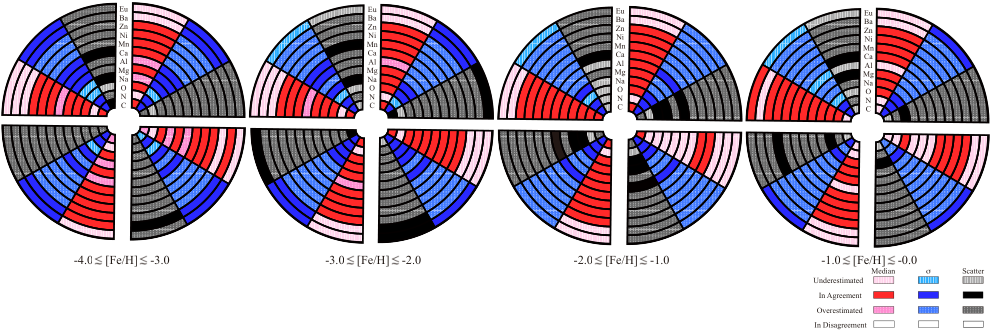
1.
The medians for single groups as well as group combinations is in good agreement with the Galactic observational data for most elements up until Zinc. However, neither the scatter nor the standard deviation of groups and group combinations tend to correlate with observational trends. Specifically, Group A and Group B underestimate most of the standard deviation and scatter of most of the data while Group C overestimates them. As for the median, Group A can predict nearly all of the data at all metallicities while Group B can predict about half of the data at all metallicities. Group C can only predict about half of the data at low metallicities and underestimates most of the data at -2.0 dex $\lesssim$ [Fe/H] $\lesssim$ 0.0 dex.
- $\bullet$
  
  Combining 2 or 3 groups at a time, the underestimated standard deviation and scatter of data only occupy a relatively small fraction at all metallicities. Although these combinations increase the fraction of the reproduced data scatter and reproduced standard deviation at low metallicities, they also increase the fraction of overestimated scatter and standard deviation. Standard deviation and scatter of data tend to be overestimated in the range -2.0 dex $\lesssim$ [Fe/H] $\lesssim$ 0.0 dex.
2.
We draw the following conclusions regarding the breakdown of elemental groups:
- $\bullet$
  
  For CNO elements, Group A and Group B underestimate most of the standard deviations of these 3 elements while Group C is in agreement with all of the standard deviations at -2.0 dex $\lesssim$ [Fe/H] $\lesssim$ 0.0 dex. Regarding the scatter, it appears that the majority of the estimates are too small for all three groups.. Most of the standard deviation of these 3 elements can be reproduced by group combinations at all metallicities.
- $\bullet$
  
  In the case of Odd-Z elements (Na and Al in our sample), we found that the median value of Na can be accurately reproduced by two of the groups. Group C performs well at lower metallicities, while it underestimates Na at -2.0 dex $\lesssim$ [Fe/H] $\lesssim$ 0.0 dex. However, Group C is in agreement with the standard deviation and most of the scatter for Na, whereas the other two groups tend to underestimate these values. In contrast to Na, Al does not exhibit clear trends.
- $\bullet$
  
  In the case of $\alpha$ elements in our sample (Mg and Ca in our sample), we found that Group A and Group B are able to reproduce most of the standard deviation and scatter of Ca, while Group C tends to overestimate these values. However, when it comes to the median of Ca, Group A and Group B are in good agreement at all metallicities, while Group C only agrees with the median at low metallicities. For Mg, both Group A and Group B tend to underestimate the standard deviation and scatter, while Group C still overestimates them. The trend for medians is similar for both Ca and Mg. In general, the median values of both Ca and Mg can be accurately reproduced for any combination of groups, although the majority of the standard deviation and scatter tend to be overestimated.
- $\bullet$
  
  Our analysis of iron-peak elements shows that Group A is able to accurately reproduce most of the median and standard deviation values of these elements at all metallicities, while Group C tends to overestimate them, as shown in Fig. 18. Group B is able to accurately reproduce the median values of these elements, with the exception of Zn, but can be in agreement with the standard deviation of Zn at -4.0 dex $\lesssim$ [Fe/H] $\lesssim$ -1.0 dex. When combining the three groups, the median values of iron-peak elements can be accurately reproduced at all metallicities, with the exception of a few data points for Zn at low metallicities. However, all of the standard deviation values for these elements tend to be overestimated by the combined groups, as shown in Fig. 19. It’s worth noting that iron-peak elements can be reproduced more accurately by the combination of the three groups than other elements, which are primarily reproduced by Group A.
- $\bullet$
  
  Neutron-capture elements (Ba and Eu), exhibit the most significant tension between observational data and theoretical models. Either single group or groups combination underestimate most of the median of Eu and Ba. As for the standard deviation, Group B and group combinations can be in agreement with most of them at low metallicities. At -2.0 dex $\lesssim$ [Fe/H] $\lesssim$ 0.0 dex, single group and groups combinations tend to overestimate Ba and underestimate Eu. As for scatter, either single group or group combination overestimate most of them.

This paper introduces statistical criteria that compare the median, standard deviation, and scatter of observational data with different groups of models, providing a measure of the ability of each yield combination to match observational data. By analyzing the effectiveness of individual yields in describing average Galactic patterns, we highlight the impact of various yield modeling assumptions on theoretical tracks. Our work shows that the abundance scatter patterns in the Milky Way cannot be explained solely by the simultaneous application of the proposed yield prescriptions.

Our objective in this analysis was to investigate whether multiple yield prescriptions and their respective scenarios could be simultaneously at play in the evolution of our Galaxy and partially responsible for the scatter of the data. We proposed statistical criteria that compares the median, standard deviation, and scatter of observational data against groups of models to evaluate the ability of each yield combination to match observational data. However, our proposed method is inconclusive due to several factors. First, a realistic mixing of yield prescriptions cannot be described by a simple average of the models without taking into account weights or time/metallicity dependence. Introducing additional modeling parameters and assumptions to describe the variation of the occurrence of each yield prescription over time would be necessary, but this goes beyond the scope of our analysis. Second, the average of evolutionary tracks is different from a single evolutionary track containing an average or mixing of the yields, with the latter being more realistic.

One-zone GCE models are appropriate for describing global evolutionary trends of elemental abundances. However, in order to analyze the spread in observational data, it is insufficient to only vary yields on a fixed galactic environment. The source of the spread in the data is likely due to varying physical or dynamical properties of the local environment, rather than the simultaneous involvement of multiple nucleosynthetic mechanisms.

While many yield prescriptions are generally effective at reproducing median Galactic trends, the inconsistency of scatter and standard deviation leads us to conclude that yield mixing may not be as significant a factor in the observed scatter of the data compared to physical properties or dynamical effects. At the same time, we cannot rule out that multiple yield prescriptions could be occurring, because several of these prescriptions are equally effective in describing average trends. To further investigate our objectives, improvements can be achieved through the use of grids of GCE models spanning a range of physical parameters, multi-zone GCE models, or hydrodynamical simulations.

Out of all the elements analyzed in this study, neutron-capture elements are the least accurately reproduced. Our analysis only accounts for merging neutron stars as an r-process enrichment channel. We therefore highlight the importance of exploring alternative production channels, such as collapsars and magneto-hydrodynamic jets.

Acknowledgements

We thank the anonymous referee for the meticulous feedback. We thank Benoit Côté for providing the complete Milky Way NuPyCEE parametrization of his 2019 work (Côté et al. 2019) and for fruitful discussions. E.G. acknowledges the support of the National Natural Science Foundation of China (NSFC) under grants NOs. 12173016, 12041305. E.G. acknowledges the science research grants from the China Manned Space Project with NOs. CMS-CSST-2021-A08, CMS-CSST-2021-A07. E.G. acknowledges the Program for Innovative Talents, Entrepreneur in Jiangsu. All the authors have been supported by the National Natural Science Foundation of China under grant (No.11922303) and the Fundamental Research Funds for the Central Universities (No.2042022kf1182).

Data Availability

No new data were generated or analysed in support of this research.

References

Abbott et al. (2017) Abbott B. P., et al., 2017, ApJ, 848, L13
Aguado et al. (2021) Aguado D. S., et al., 2021, ApJ, 908, L8
Aliotta et al. (2022) Aliotta M., et al., 2022, Journal of Physics G Nuclear Physics, 49, 010501
Ananna et al. (2022) Ananna C., et al., 2022, Universe, 8
Andrews et al. (2017) Andrews B. H., Weinberg D. H., Schönrich R., Johnson J. A., 2017, ApJ, 835, 224
Arcones & Thielemann (2023) Arcones A., Thielemann F.-K., 2023, A&ARv, 31, 1
Argast et al. (2004) Argast D., Samland M., Thielemann F. K., Qian Y. Z., 2004, A&A, 416, 997
Asplund et al. (2009) Asplund M., Grevesse N., Sauval A. J., Scott P., 2009, ARA&A, 47, 481
Bensby & Feltzing (2006) Bensby T., Feltzing S., 2006, MNRAS, 367, 1181
Bensby et al. (2005) Bensby T., Feltzing S., Lundström I., Ilyin I., 2005, A&A, 433, 185
Bensby et al. (2014) Bensby T., Feltzing S., Oey M. S., 2014, A&A, 562, A71
Bensby et al. (2017) Bensby T., et al., 2017, A&A, 605, A89
Bethe (1939) Bethe H. A., 1939, Physical Review, 55, 434
Boyer et al. (2012) Boyer M. L., et al., 2012, ApJ, 748, 40
Buchmann & Barnes (2006) Buchmann L. R., Barnes C. A., 2006, Nuclear Phys. A, 777, 254
Burbidge et al. (1957) Burbidge E. M., Burbidge G. R., Fowler W. A., Hoyle F., 1957, Reviews of Modern Physics, 29, 547
Cameron (1957) Cameron A. G. W., 1957, PASP, 69, 201
Carretta et al. (2000) Carretta E., Gratton R. G., Sneden C., 2000, A&A, 356, 238
Cayrel et al. (2004) Cayrel R., et al., 2004, A&A, 416, 1117
Cescutti (2008) Cescutti G., 2008, A&A, 481, 691
Cescutti et al. (2006) Cescutti G., François P., Matteucci F., Cayrel R., Spite M., 2006, A&A, 448, 557
Chen et al. (2022) Chen B., Hayden M. R., Sharma S., Bland-Hawthorn J., Kobayashi C., Karakas A. I., 2022, arXiv e-prints, p. arXiv:2204.11413
Clayton (2003) Clayton D., 2003, Handbook of Isotopes in the Cosmos. Cambridge University Press
Côté et al. (2016) Côté B., West C., Heger A., Ritter C., O’Shea B. W., Herwig F., Travaglio C., Bisterzo S., 2016, MNRAS, 463, 3755
Côté et al. (2017) Côté B., O’Shea B. W., Ritter C., Herwig F., Venn K. A., 2017, ApJ, 835, 128
Côté et al. (2019) Côté B., et al., 2019, ApJ, 875, 106
Cowan & Thielemann (2004) Cowan J. J., Thielemann F.-K., 2004, Physics Today, 57, 10.47
Cristallo et al. (2011) Cristallo S., et al., 2011, ApJS, 197, 17
Cristallo et al. (2015) Cristallo S., Straniero O., Piersanti L., Gobrecht D., 2015, ApJS, 219, 40
Dearborn et al. (1978) Dearborn D. S. P., Tinsley B. M., Schramm D. N., 1978, ApJ, 223, 557
Fields et al. (2018) Fields C. E., Timmes F. X., Farmer R., Petermann I., Wolf W. M., Couch S. M., 2018, ApJS, 234, 19
Freer & Fynbo (2014) Freer M., Fynbo H. O. U., 2014, Progress in Particle and Nuclear Physics, 78, 1
Fröhlich et al. (2006) Fröhlich C., et al., 2006, ApJ, 637, 415
Fryer et al. (2012) Fryer C. L., Belczynski K., Wiktorowicz G., Dominik M., Kalogera V., Holz D. E., 2012, ApJ, 749, 91
Gail et al. (2009) Gail H. P., Zhukovska S. V., Hoppe P., Trieloff M., 2009, ApJ, 698, 1136
Gilmore et al. (2012) Gilmore G., et al., 2012, The Messenger, 147, 25
Hawkins et al. (2020) Hawkins K., et al., 2020, MNRAS, 492, 1164
Haynes & Kobayashi (2019) Haynes C. J., Kobayashi C., 2019, MNRAS, 483, 5123
Hoyle (1954) Hoyle F., 1954, ApJS, 1, 121
Israelian et al. (2004) Israelian G., Ecuvillon A., Rebolo R., García-López R., Bonifacio P., Molaro P., 2004, A&A, 421, 649
Iwamoto et al. (1999) Iwamoto K., Brachwitz F., Nomoto K., Kishimoto N., Umeda H., Hix W. R., Thielemann F.-K., 1999, ApJS, 125, 439
Johnson et al. (2021) Johnson J. W., et al., 2021, MNRAS, 508, 4484
Jones et al. (2015) Jones S., Hirschi R., Pignatari M., Heger A., Georgy C., Nishimura N., Fryer C., Herwig F., 2015, MNRAS, 447, 3115
Karakas (2010) Karakas A. I., 2010, MNRAS, 403, 1413
Kibédi et al. (2020) Kibédi T., et al., 2020, Phys. Rev. Lett., 125, 182701
Kobayashi et al. (2006) Kobayashi C., Umeda H., Nomoto K., Tominaga N., Ohkubo T., 2006, ApJ, 653, 1145
Kobayashi et al. (2011) Kobayashi C., Tominaga N., Nomoto K., 2011, ApJ, 730, L14
Kobayashi et al. (2020) Kobayashi C., Karakas A. I., Lugaro M., 2020, ApJ, 900, 179
Kobayashi et al. (2023) Kobayashi C., et al., 2023, ApJ, 943, L12
Kroupa (2001) Kroupa P., 2001, MNRAS, 322, 231
Kroupa et al. (2020) Kroupa P., Haslbauer M., Banik I., Nagesh S. T., Pflamm-Altenburg J., 2020, MNRAS, 497, 37
Kunz et al. (2002) Kunz R., Fey M., Jaeger M., Mayer A., Hammer J. W., Staudt G., Harissopulos S., Paradellis T., 2002, ApJ, 567, 643
Lattimer & Schramm (1974) Lattimer J. M., Schramm D. N., 1974, ApJ, 192, L145
Limongi & Chieffi (2018) Limongi M., Chieffi A., 2018, ApJS, 237, 13
Maeda et al. (2010) Maeda K., Röpke F. K., Fink M., Hillebrandt W., Travaglio C., Thielemann F. K., 2010, ApJ, 712, 624
Maeder & Meynet (2000) Maeder A., Meynet G., 2000, A&A, 361, 159
Martin (1999) Martin C. L., 1999, ApJ, 513, 156
Mashonkina et al. (2017) Mashonkina L., Jablonka P., Sitnova T., Pakhomov Y., North P., 2017, A&A, 608, A89
Matteucci (1986) Matteucci F., 1986, MNRAS, 221, 911
Matteucci (2001) Matteucci F., 2001, The chemical evolution of the Galaxy. Astrophysics and space science library Vol. 253, Kluwer Academic Publisher, doi:10.1007/978-94-010-0967-6
Matteucci (2012) Matteucci F., 2012, Chemical Evolution of Galaxies. Astronomy and Astrophysics Library. Springer-Verlag Berlin Heidelberg, doi:10.1007/978-3-642-22491-1
Matteucci (2021) Matteucci F., 2021, A&ARv, 29, 5
Matteucci et al. (2009) Matteucci F., Spitoni E., Recchi S., Valiante R., 2009, A&A, 501, 531
Meynet & Maeder (2002) Meynet G., Maeder A., 2002, A&A, 390, 561
Murray et al. (2005) Murray N., Quataert E., Thompson T. A., 2005, ApJ, 618, 569
Nieva & Przybilla (2012) Nieva M. F., Przybilla N., 2012, A&A, 539, A143
Nissen (2016) Nissen P. E., 2016, A&A, 593, A65
Nomoto et al. (1984) Nomoto K., Thielemann F. K., Yokoi K., 1984, ApJ, 286, 644
Nomoto et al. (2013) Nomoto K., Kobayashi C., Tominaga N., 2013, ARA&A, 51, 457
Pagel (2009) Pagel B. E. J., 2009, Nucleosynthesis and Chemical Evolution of Galaxies. Cambridge University Press
Pagel & Tautvaisiene (1997) Pagel B. E. J., Tautvaisiene G., 1997, MNRAS, 288, 108
Palla et al. (2022) Palla M., Santos-Peral P., Recio-Blanco A., Matteucci F., 2022, A&A, 663, A125
Paxton et al. (2011) Paxton B., Bildsten L., Dotter A., Herwig F., Lesaffre P., Timmes F., 2011, ApJS, 192, 3
Paxton et al. (2015) Paxton B., et al., 2015, ApJS, 220, 15
Prantzos et al. (2018) Prantzos N., Abia C., Limongi M., Chieffi A., Cristallo S., 2018, MNRAS, 476, 3432
Prantzos et al. (2020) Prantzos N., Abia C., Cristallo S., Limongi M., Chieffi A., 2020, MNRAS, 491, 1832
Reddy et al. (2003) Reddy B. E., Tomkin J., Lambert D. L., Allende Prieto C., 2003, MNRAS, 340, 304
Reddy et al. (2006) Reddy B. E., Lambert D. L., Allende Prieto C., 2006, MNRAS, 367, 1329
Reggiani et al. (2017) Reggiani H., Meléndez J., Kobayashi C., Karakas A., Placco V., 2017, A&A, 608, A46
Ritter et al. (2018) Ritter C., Herwig F., Jones S., Pignatari M., Fryer C., Hirschi R., 2018, MNRAS, 480, 538
Roederer et al. (2014) Roederer I. U., Preston G. W., Thompson I. B., Shectman S. A., Sneden C., Burley G. S., Kelson D. D., 2014, AJ, 147, 136
Romano (2022) Romano D., 2022, A&ARv, 30, 7
Romano et al. (2010) Romano D., Karakas A. I., Tosi M., Matteucci F., 2010, A&A, 522, A32
Romano et al. (2019) Romano D., Matteucci F., Zhang Z.-Y., Ivison R. J., Ventura P., 2019, MNRAS, 490, 2838
Romano et al. (2020) Romano D., Franchini M., Grisoni V., Spitoni E., Matteucci F., Morossi C., 2020, A&A, 639, A37
Rybizki et al. (2017) Rybizki J., Just A., Rix H.-W., 2017, A&A, 605, A59
Salpeter (1952) Salpeter E. E., 1952, ApJ, 115, 326
Schombert et al. (2019) Schombert J., McGaugh S., Lelli F., 2019, MNRAS, 483, 1496
Schönrich & Binney (2009) Schönrich R., Binney J., 2009, MNRAS, 396, 203
Seitenzahl et al. (2013) Seitenzahl I. R., et al., 2013, MNRAS, 429, 1156
Shen et al. (2015) Shen S., Cooke R. J., Ramirez-Ruiz E., Madau P., Mayer L., Guedes J., 2015, ApJ, 807, 115
Shibagaki et al. (2016) Shibagaki S., Kajino T., Mathews G. J., Chiba S., Nishimura S., Lorusso G., 2016, ApJ, 816, 79
Siegel et al. (2019) Siegel D. M., Barnes J., Metzger B. D., 2019, Nature, 569, 241
Smartt et al. (2017) Smartt S. J., et al., 2017, Nature, 551, 75
Smiljanic et al. (2016) Smiljanic R., et al., 2016, A&A, 589, A115
Spitoni et al. (2015) Spitoni E., Romano D., Matteucci F., Ciotti L., 2015, ApJ, 802, 129
Spitoni et al. (2020) Spitoni E., Verma K., Silva Aguirre V., Calura F., 2020, A&A, 635, A58
Spitoni et al. (2021) Spitoni E., et al., 2021, A&A, 647, A73
Suess & Urey (1956) Suess H. E., Urey H. C., 1956, Reviews of Modern Physics, 28, 53
Talbot & Arnett (1974) Talbot R. J. J., Arnett D. W., 1974, ApJ, 190, 605
Thielemann et al. (1986) Thielemann F. K., Nomoto K., Yokoi K., 1986, A&A, 158, 17
Thielemann et al. (1996) Thielemann F.-K., Nomoto K., Hashimoto M.-A., 1996, ApJ, 460, 408
Thielemann et al. (2017) Thielemann F. K., Eichler M., Panov I. V., Wehmeyer B., 2017, Annual Review of Nuclear and Particle Science, 67, 253
Tinsley (1979) Tinsley B. M., 1979, ApJ, 229, 1046
Travaglio et al. (2011) Travaglio C., Röpke F. K., Gallino R., Hillebrandt W., 2011, ApJ, 739, 93
Trueman et al. (2022) Trueman T. C. L., Côté B., Yagüe López A., den Hartogh J., Pignatari M., Soós B., Karakas A. I., Lugaro M., 2022, ApJ, 924, 10
Truran & Cameron (1971) Truran J. W., Cameron A. G. W., 1971, Ap&SS, 14, 179
Truran & Heger (2003) Truran J. W. J., Heger A., 2003, Treatise on Geochemistry, 1, 711
Vangioni et al. (2018) Vangioni E., Dvorkin I., Olive K. A., Dubois Y., Molaro P., Petitjean P., Silk J., Kimm T., 2018, MNRAS, 477, 56
Veilleux et al. (2005) Veilleux S., Cecil G., Bland-Hawthorn J., 2005, ARA&A, 43, 769
Ventura et al. (2013) Ventura P., Di Criscienzo M., Carini R., D’Antona F., 2013, MNRAS, 431, 3642
Ventura et al. (2014a) Ventura P., di Criscienzo M., D’Antona F., Vesperini E., Tailo M., Dell’Agli F., D’Ercole A., 2014a, MNRAS, 437, 3274
Ventura et al. (2014b) Ventura P., Dell’Agli F., Schneider R., Di Criscienzo M., Rossi C., La Franca F., Gallerani S., Valiante R., 2014b, MNRAS, 439, 977
Wallerstein (1962) Wallerstein G., 1962, ApJS, 6, 407
Watson et al. (2019) Watson D., et al., 2019, Nature, 574, 497
Weinberg et al. (2017) Weinberg D. H., Andrews B. H., Freudenburg J., 2017, ApJ, 837, 183
Wiescher et al. (2010) Wiescher M., Görres J., Uberseder E., Imbriani G., Pignatari M., 2010, Annual Review of Nuclear and Particle Science, 60, 381
Woosley & Weaver (1995) Woosley S. E., Weaver T. A., 1995, ApJS, 101, 181
Woosley et al. (2002) Woosley S. E., Heger A., Weaver T. A., 2002, Reviews of Modern Physics, 74, 1015
Yamazaki et al. (2022) Yamazaki Y., He Z., Kajino T., Mathews G. J., Famiano M. A., Tang X., Shi J., 2022, ApJ, 933, 112
Yan et al. (2019) Yan Z., Jerabkova T., Kroupa P., Vazdekis A., 2019, A&A, 629, A93
Zhao et al. (2016) Zhao G., et al., 2016, ApJ, 833, 225
van de Voort et al. (2020) van de Voort F., Pakmor R., Grand R. J. J., Springel V., Gómez F. A., Marinacci F., 2020, MNRAS, 494, 4867