HybridCVLNet: A Hybrid CSI Feedback System and its Domain AdaptationThanks: This work has been submitted to the IEEE for possible publication. Copyright may be transferred without notice, after which this version may no longer be accessible.Thanks: H. Li, B. Zhang, D. Li, Z. Liu, L. Zhang are with the School of Artificial Intelligence, Beijing University of Posts and Telecommunications, Beijing, 100876, China (e-mail: {lihaozhen, zhangboyuan, rhyme_lee, lzyu, zhanglin}@bupt.edu.cn). X. Gu is with the School of Artificial Intelligence, Beijing University of Posts and Telecommunications, Beijing, 100876, China. She is also with the Purple Mountain Laboratories, Nanjing 211111, China (e-mail: guxinyu@bupt.edu.cn).

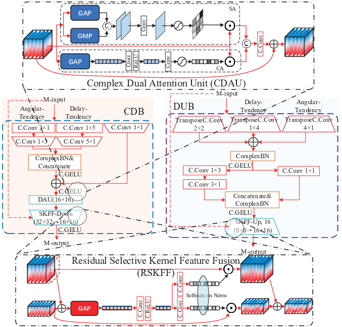
The HybridCVLNet adopts the cascading complex-valued Convolutional Down-sampling Block (CDB) and Deconvolutional Up-sampling Block (DUB) that can efficiently embed phase information into the latent with the inductive bias of translation equivariance [25], illustrated in Fig. 5. The self-attention mechanism weighs the input feature by defining how important (i.e. attention scores) an element is and from which dimensions (i.e. interactions) to judge. The HybridCVLNet derives an attention-score calculation for complex-valued features with interpretability and proposes multiple methods to apply it.

Given a complex-valued feature map $\mathbf{M}\in\mathbb{C}^{K\times H\times W}$, the self-attentiveness of element $\mathbf{m}_{h,w}$ of tensor $\mathbf{M}$ is quantified by the L2 norm value $\|\mathbf{m}_{h,w}\|_{2}$. The attentiveness can be utilized to calculate the attention scores, formulated as

that is regarded as a transformation from two discrete variables $\mathfrak{R}(\mathbf{m}_{h,w})$ and $\mathfrak{I}(\mathbf{m}_{h,w})$ to the distance away from the original point in the complex plane. Considering the sparsity of complex-valued ADCRM, the distance $\|\mathbf{m}_{h,w}\|_{2}$ intuitively describes the intensity of element $\mathbf{m}_{h,w}$. To increase the interpretability, the $\|\mathbf{m}_{h,w}\|_{2}$ is equivalent to the tap amplitude of wireless channel delay profile $|\mathbf{h}(t,\tau)|$, where $\mathbf{h}(t,\tau)=\sum_{i=1}^{N}{c_{i}\left(t\right)\delta\left(\tau-\tau_{i}\right)}$. Note that the impulse response $\mathbf{h}$ and the multipath component coefficient $c_{i}\left(t\right)$ varies with time $t$, representing the channel by a delay line with $N$ taps.

The complex-valued self-attention on $\mathbf{M}$ can be exploited either with inter-channel or with inter-spatial interactions. A global pooling operation obtains a descriptor $\mathbf{d}_{\text{inter-channel}}\in\mathbb{R}^{K\times 1\times 1}$ or $\mathbf{d}_{\text{inter-spatial}}\in\mathbb{R}^{1\times H\times W}$ adopts on $\|\mathbf{m}_{h,w}\|_{2}$ across spatial dimension or channel dimension, which is lately activated through a convolutional layer followed by the Sigmoid gating. Motivated by the SOTA self-attention application [28], the HybridCVLNet embeds a Complex Dual Attention Unit (CDAU), as shown in the upper zoom-in area of Fig. 5 that suppresses less-useful while passing the more informative features. To promote multi-scale features interaction and receptive field variation of the [29], a Residual Selective Kernel Feature Fusion (RSKFF) block with multi-scale fusing and inter-channel self-attention is proposed, illustrated in the lower zoom-in area of Fig. 5.

When inter-domain data drift appears, preserving the validity of the HybridCVLNet discriminative branch, i.e., the prior regularity information, can be helpful. The AdaMatch [31] is a categorical DA scheme that constrains the source and target domain logits $\mathbf{d}_{\text{CL},SL}$ and $\mathbf{d}_{\text{CL},TU}$ with distribution alignment, which encourages the target pseudo-labels in target distribution $\mathbb{P}_{TU}$ to follow the source label distribution $\mathbb{P}_{SL}$. We conduct an MLC version of AdaMatch (ML-AdaMatch) so that the target SH features $\mathbf{x}_{\text{SH},SL}$ are still category-related, and $\mathbf{d}_{\text{CL},TU}$ is valid, while the target domain is unknown.

We concatenate the source and target domain batch together, denoted as $\mathcal{X}_{\mathcal{D}}=\{\mathcal{X}_{SL},\mathcal{X}_{TU}\}$. We then compute logits $\mathbf{y}_{SL}^{\prime}$, $\mathbf{y}_{SL}^{{}^{\prime\prime}\mkern-1.2mu}$ and $\mathbf{y}_{TU}$ as follows:

notably, we utilize batch normalization as the adapter to the target distribution. Thus, only batch normalization is updated at the second forward propagation. We randomly interpolating the logits $\mathbf{y}_{SL}^{\prime}$ and $\mathbf{y}_{SL}^{{}^{\prime\prime}\mkern-1.2mu}$ to obtain source-domain logits $\mathbf{y}_{SL}$ as follow,

where $\lambda_{\text{RI}_{\text{ENV}}}\sim\mathcal{U}^{n_{SL}\cdot 2}(0,1)$ and $\lambda_{\text{RI}_{\text{DP}}}\sim\mathcal{U}^{n_{SL}\cdot 5}(0,1)$ for channel environment and CDL delay profiles. This formulation implicitly does $\underset{W_{\text{MLC}}}{\min}\left|\mathbf{y}_{SL}^{\prime}-\mathbf{y}_{SL}^{{}^{\prime\prime}\mkern-1.2mu}\right|$. We approximate the unknown $\mathbb{P}_{TU}$ using the closest available distribution $\mathbb{P}_{SL}$ that aligns the statistical property of $\mathbf{y}_{TU}=\{\mathbf{y}_{TU_{\text{DP}}},\mathbf{y}_{TU_{\text{ENV}}}\}$ with $\mathbf{y}_{SL}=\{\mathbf{y}_{SL_{\text{DP}}},\mathbf{y}_{SL_{\text{ENV}}}\}$ that helps significantly with the discriminative effectiveness [31].

Then, we compute pseudo labels with softmax activation $\widehat{\mathbf{y}}_{SL_{\text{DP}}}$, $\widehat{\mathbf{y}}_{SL_{\text{ENV}}}$ and $\widehat{\mathbf{y}}_{TU_{\text{DP}}}$, $\widehat{\mathbf{y}}_{TU_{\text{ENV}}}$ separately. The distribution alignment rectifies the target unlabeled pseudo-labels by multiplying with the ratio of the expected value to obtain the final pseudo-labels ${\widetilde{\mathbf{y}}}_{TU}\in\mathbb{R}^{n_{TU}\times 7}$,

the $\text{normalize}(\cdot)$ ensures that the logits sums to 1. As could be seen along the optimization, $\mathbb{E}\left[{\widetilde{\mathbf{y}}}_{TU}\right]=\mathbb{E}\left[{\widehat{\mathbf{y}}}_{SL}\right]$ confirms that distribution alignment makes the target pseudo-labels follow the source label distribution.

To selectively utilize the aligned target pseudo logits, a multi-label confidence threshold on user-provided value $\tau_{\text{CT}}$ is proposed. The relative confidence threshold $c_{\tau_{\text{CT}}}$ and binary mask $\mathbf{v}\in\left\{0,1\right\}^{n_{TU}}$ defined as follows,

The loss function $\mathcal{L}_{\text{DA}}$ sums $\mathcal{L}_{\text{DA}_{SL}}$ for the source and $\mathcal{L}_{\text{DA}_{TU}}$ for the target.

where $\text{Eval}(\cdot)$ is the evaluation mode of model. The $\mu(t)$ is a warmup function that controls $\mathcal{L}_{\text{DA}_{TU}}$ at every step of the training, which smoothly raises from zero to one for the first half of the training and remains at one for the second half [31].

GAN-based image compression system synthesizes details in the limit-bandwidth scenario, obtaining visually pleasing results and showing strong artefacts [32] [33]. The HybridCVLNet adopts a lightweight discriminator and introduces the adversarial term to the DA stage to stimulate the adaptation to the target domain in the CSI feature space.

Given a dataset $\mathcal{D}_{\mathbf{x}}$, original GANs learn to approximate distribution $\mathbb{P}_{\mathbf{x}}$ through a generator $G\left(\mathbf{z}\right)$ that maps samples $\mathbf{z}$ from a prior distribution $\mathbb{P}_{z}$ to the data distribution $\mathbb{P}_{\mathbf{x}}$. The generator $G$ is trained in parallel with a discriminator $Dis$ with the objective as follows,

where $f$ and $g$ are scalar functions to solve $\underset{G}{\text{min}}{\mathcal{L}_{\text{GAN}}}$ that allows to minimize general $f$-divergences between the distribution of $G(\mathbf{z})$ and $\mathbb{P}_{\mathbf{x}}$. The compression GANs (CG) for CSI feedback [9] can be viewed as a combination of GANs and deep compression. Given latent $\mathbf{s}=E\left(\mathbf{H}\right)$, where encoder $E=\{g_{\text{SH}},g_{\text{SH}_{\text{D}}}\circ g_{\text{UH}},g_{\text{UH}_{\text{D}}}\}$, the saddle-point objective for GAN-based CSI feedback is formulated as,

where $G$ is the Generator, $G=\{g_{\text{GT}},g_{\text{GT}_{\text{D}}}\circ g_{\text{RT}},g_{\text{RT}_{\text{D}}}\circ g_{\text{RB}}\}$, $\lambda_{\text{adv}}$ is the hyperparameter determines the balance between the generation and reconstruction and $d$ measures reconstruct similarity (i.e., $\ell_{r}$).

In domain adaptation, given source image and label pairs $(\mathcal{X}_{SL},\mathcal{Y}_{SL})\sim\mathbb{P}_{SL}$ and target images $\mathcal{X}_{TU}\sim\mathbb{P}_{TU}$. In a typical unsupervised domain adaptation (UDA) scheme that learns the source and target mapping $f_{SL}$ and $f_{TU}$ to minimize the difference of feature $f_{SL}(\mathcal{X}_{SL})$ and $f_{TU}(\mathcal{X}_{TU})$ in processing by the discriminate of the domain discriminator $Dis$. Substantially different, the primary goal of the CSI feedback is to achieve CSI regression ($f_{r}$). However, existing UDA schemes focus on intermediate features $\mathbf{M}_{SL}^{I}$, $\mathbf{M}_{TU}^{I}$ may not contribute. Thus a CSI feature-space stimulation DA is proposed to adapt with the $\mathbb{P}_{TU}$ as,

where $f_{\text{LSGAN}}(\mathbf{y})={(\mathbf{y}-1)}^{2}$ and $g_{\text{LSGAN}}\left(\mathbf{y}\right)=\mathbf{y}^{2}$ (which corresponds to the Pearson $\mathcal{X}^{2}$ divergence) in [34] to overcome the vanishing gradients problem of regular GANs, $\mathbf{s}_{TU}$ is the codeword of target domain sample. A verified CDB with anti-alias downsampling (max) and an anti-alias downsampling (average) branch [35] is adopted as the $Dis$.

Furthermore, inspired by the SOTA CG with a semantic mask that could fully synthesize unimportant regions [2]. innovatively, a polar-star-like binary mask $\mathbf{M}_{\text{polar}}$ that indicates the emphasis region to synthesize is proposed. It firstly masks the $\mathbf{d}_{\text{SI}}$ sequence, and considering the amplitude fluctuation around the scatterer location is critical in final regression, a square mask $\mathbf{M}_{\text{square}}\in\mathbb{R}^{3\times 3}$ is assigned. Meanwhile, a delay-direction and angular-direction masks $\mathbf{M}_{\text{delay}}\in\mathbb{R}^{1\times 9}$ and $\mathbf{M}_{\text{angular}}\in\mathbb{R}^{7\times 1}$ are appended to the $\mathbf{M}_{\text{polar}}=\left\{\mathbf{M}_{\text{square}},\mathbf{M}_{\text{delay}},\mathbf{M}_{\text{angular}}\right\}$. The masked GT block feature $\mathbf{M}_{{\text{GT}}}=\mathbf{M}_{\text{polar}}\odot\mathbf{M}_{\text{GT}}$ of HybridCVLNet assigns the regions of zeros corresponding to the area that should be synthesized, and regions of ones should be preserved to promote the masked region adaptation of each CSI sample. We believe such a semantic mask can facilitate adaptation to the CSI amplitude fluctuation pattern of the target domain.

The objective of HybridCLVNet HDA is a three parts combination, namely the primary target regression objective $\mathcal{L}_{\text{r}}$ from (15), the distribution-alignment objective $\mathcal{L}_{\text{DA}}$ from ML-AdaMatch loss formula (25), and the adversarial generative objective $\mathcal{L}_{\text{adv}}$ in (28). We define three hyperparameters $\lambda_{\text{Content}}$, $\lambda_{\text{Rug}_{\text{HDA}}}$, and $\lambda_{\text{adv}}$ to weight each term respectively and the total learning objective is defined as follows,

An inductive-based adaptation to the target domain of a Vanilla CSI feedback system is shown in Fig. 10(a), which gradually adapted with $\mathcal{L}_{\text{r}}$, yet the source domain inference performance may have an unavoidable degradation, namely the "catastrophic forgetting". Similarly, the HybridCVLNet adapted to the target domain with only $\mathcal{L}_{\text{r}}$ would forfeit prior regularized distribution knowledge, as shown in Fig. 10(b) that ruins the category-related functions ($f_{c}$ and $f_{s}$) of HybridCVLNet. To preserve the prior regularization, we introduce the $\mathcal{L}_{\text{DA}}$ of (25), as shown in the central of Fig. 10(b), and from the view of feature, the adversarial generative loss stimulation $\mathcal{L}_{\text{Fadv}}$ in (28) is leveraged as shown in the right of Fig. 10(b) to mimic the patterns of the target domain in artefact space.

The optimization strategy of HybridCVLNet HDA is to promote primary target regression optimization and preserve the prior classification latent simultaneously, as shown in Fig. 10(c). To simplify the hyperparameters, we set the $\lambda_{\text{Content}}=1$, and adjust the balance between the adversarial generative $\mathcal{L}_{\text{Fadv}}$ and distribution alignment terms $\mathcal{L}_{\text{DA}}$ with two ratio factors $\lambda_{\text{Rug}_{\text{HDA}}}$ and $\lambda_{\text{adv}}$. Theoretically, the $\mathcal{L}_{\text{DA}}$ is more effective when target and source category distribution are similar. Increasing $\lambda_{\text{Rug}_{\text{HDA}}}$ maintains the category-related performance. In comparison, increasing $\lambda_{\text{adv}}$ motivates the feature-space regression to the target domain.

In this experiment, we evaluate the performance of the HybridCVLNet with its learning objective on the heterogeneous regularization dataset. As the theoretical design, the proposed HybridCVLNet can effectively preserve the category-related features and fuse with category-invariant features for refinement. The challenge is to obtain guaranteed regression manifestation (achieves the $f_{r}$) and high classification accuracy (achieves the $f_{c}$) simultaneously.

The dataset $\mathcal{D}_{SL}$ is generated on the CDL channel model described in Section IV with parameter settings shown in Table IV in a perfect downlink channel estimation mode to obtain $\mathbf{H}\in\mathbb{C}^{2\times 32\times 612}$. Latterly was processed with domain transformation to ADCRM, where the angular resolution sampling point is chosen as the number of antennas, and the delay sample point is 400 to obtain $\mathbf{H}_{\text{AD}}\in\mathbb{C}^{2\times 32\times 400}$. Considering the channel sparsity in the large delay range, the $\mathbf{H}_{\text{AD}}$ is truncated to 32 along the delay axis that $\mathbf{H}_{\text{AD}}^{\prime}\in\mathbb{C}^{2\times 32\times 32}$, and is normalized with the mean value of $0.5$ by min-max normalization. The $\mathcal{D}_{SL}$ randomly shuffled five types of CDL delay profiles from CDL-A to E, and $30\%$ of the category-balanced dataset is chosen for testing ($N_{\text{train}}=112,000$ and $N_{\text{test}}=48,000$).

Several Key Performance Indicators (KPIs) are considered for the thorough assessment. The regression task $f_{r}$ of HybridCVLNet conducts the global normalized mean squared error (NMSE) as the intra-domain heterogeneous CSI reconstruction quality metric. The regularization task $f_{c}$ adopts the overall and per-category F1-measure (OF1 and CF1) to evaluate the classification accuracy. The expression of NMSE in decibels (dB) is given by:

alternatively, the OF1 and CF1 between the final logits $\widehat{\mathbf{y}}$ and the target label $\mathbf{y}$ defined as

To be fair in revealing the performance of the proposed HybridCVLNet, based on the discussion of the critical factors of deep learning generalizability, we list the performance comparison among original benchmark CsiNet [5] that balanced between performance and parameters, the SOTA performance-seeking CRNet [14], the benchmark lightweight CLNet [36] with extreme low parameter and complexity, and the SOTA complex-valued CVLNet [37]. In particular, to the best of our knowledge, there is no related literature on CSI feedback that utilizes discriminative tasks to regularize. The PRVNet [10], as a VAE CSI feedback scheme, is considered an effective partial regularity scheme that uses the KL-divergence loss term. Nevertheless, it is not convergent in the heterogeneous dataset $\mathcal{D}_{SL}$.

The HybridCVLNet follows a balanced learning strategy and sets the hyperparameters $\lambda_{\text{Rug}}$ of the objective function (15) to $1e^{-3}$. The feature-augmentation is involved when the discriminative $\mathcal{L}_{\text{c}}$ and regression $\mathcal{L}_{\text{r}}$ terms of (15) are convergence smoothly. Thus we set the $\bm{Epoch}_{\text{Ar}}\in{\{70,...,150\}}$.

Table III summarizes the overall performance comparison. The network size is measured by total (UE and BS side) parameter numbers directly indicating the model size. The HybridCVLNet can achieve a significant parameter reduction of about $72.9\%$ when $\gamma=1/4$, $66.6\%$ when $\gamma=1/8$, $57.7\%$ and $47.2\%$ when $\gamma=1/16$ and $\gamma=1/32$ with a stable advantage on inference, respectively. Our parametric advantage comes mainly from the CDB and UDB that process features while mapping. In addition, lightweight design throughout the HybridCVLNet, such as depthwise separable convolution and layer normalization from RFA, the inverse bottleneck structure. We also calculate the network complexity with the floating-point operations per second (FLOPs) of the HybridCVLNet, which is $26.3$M when $\gamma=1/16$ that is competitive with SOTA lightweight CSI feedback system [38] with $24.3$M of UE side. We believe that the lightweight structure of HybridCVLNet offers the possibility of improving the generalizability of the system, which is also in line with the conventional neural network generalization theory.

References

- [1] L. Theis, W. Shi, A. Cunningham, and F. Huszár, “Lossy Image Compression with Compressive Autoencoders,” arXiv e-prints, p. arXiv:1703.00395, Mar. 2017.
- [2] J. Ballé, D. Minnen, S. Singh, S. J. Hwang, and N. Johnston, “Variational image compression with a scale hyperprior,” arXiv e-prints, p. arXiv:1802.01436, Jan. 2018.
- [3] J. Guo, C.-K. Wen, S. Jin, and G. Y. Li, “Overview of deep learning-based CSI feedback in massive MIMO systems,” IEEE Trans. Commun., vol. 70, no. 12, pp. 8017–8045, Oct. 2022.
- [4] J. Guo, C.-K. Wen, S. Jin, and X. Li, “AI for CSI Feedback Enhancement in 5G-Advanced,” arXiv e-prints, p. arXiv:2206.15132, Jun. 2022.
- [5] C.-K. Wen, W.-T. Shih, and S. Jin, “Deep learning for massive MIMO CSI feedback,” IEEE Wireless Commun. Lett., vol. 7, no. 5, pp. 748–751, Oct. 2018.
- [6] H. Li, B. Zhang, X. Liang, H. Chang, X. Gu, and L. Zhang, “CSI Sensing and Feedback: A Semi-Supervised Learning Approach,” arXiv e-prints, p. arXiv:2110.06142, Sep. 2021.
- [7] B. Zhang, H. Li, X. Liang, X. Gu, and L. Zhang, “Multi-task training approach for CSI feedback in massive MIMO systems,” IEEE Commun. Lett., vol. 27, no. 1, pp. 200–204, Oct. 2023.
- [8] Y. Lu and J. Lu, “A universal approximation theorem of deep neural networks for expressing probability distributions,” Proc. NIPS, vol. 33, pp. 3094–3105, 2020.
- [9] B. Tolba, M. Elsabrouty, M. G. Abdu-Aguye, H. Gacanin, and H. M. Kasem, “Massive MIMO CSI feedback based on generative adversarial network,” IEEE Commun. Lett., vol. 24, no. 12, pp. 2805–2808, Aug. 2020.
- [10] M. Hussien, K. K. Nguyen, and M. Cheriet, “PRVNet: A novel partially-regularized variational autoencoders for massive MIMO CSI feedback,” in 2022 IEEE Wireless Commun. Netw. Conf. (WCNC), Apr. 2022, pp. 2286–2291.
- [11] S. Jo and J. So, “Adaptive lightweight cnn-based CSI feedback for massive MIMO systems,” IEEE Wireless Commun. Lett., vol. 10, no. 12, Oct. 2021.
- [12] J. Guo, C.-K. Wen, S. Jin, and G. Y. Li, “Convolutional neural network-based multiple-rate compressive sensing for massive MIMO CSI feedback: Design, simulation, and analysis,” IEEE Trans. Wireless Commun., vol. 19, no. 4, pp. 2827–2840, Jan. 2020.
- [13] Z. Hu, J. Guo, G. Liu, H. Zheng, and J. Xue, “MRFNet: A deep learning-based CSI feedback approach of massive MIMO systems,” IEEE Commun. Lett., vol. 25, no. 10, pp. 3310–3314, Jul. 2021.
- [14] Z. Lu, J. Wang, and J. Song, “Multi-resolution CSI feedback with deep learning in massive MIMO system,” in ICC 2020 - 2020 IEEE Int. Conf. Commun. (ICC), Jun. 2020, pp. 1–6.
- [15] Y. Zhang, J. Wang, J. Sun, B. Adebisi, H. Gacanin, G. Gui, and F. Adachi, “CV-3DCNN: Complex-valued deep learning for CSI prediction in FDD massive MIMO systems,” IEEE Wireless Commun. Lett., vol. 10, no. 2, pp. 266–270, Sep. 2021.
- [16] J. Zeng, J. Sun, G. Gui, B. Adebisi, T. Ohtsuki, H. Gacanin, and H. Sari, “Downlink CSI feedback algorithm with deep transfer learning for FDD massive MIMO systems,” IEEE Trans. on Cognitive Communications and Networking, vol. 7, no. 4, pp. 1253–1265, 2021.
- [17] Y. Mitsuzumi, G. Irie, D. Ikami, and T. Shibata, “Generalized domain adaptation,” in Proc. IEEE Conf. Comput. Vis. Pattern Recognit. (CVPR), Jun. 2021, pp. 1084–1093.
- [18] P. Li, D. Li, W. Li, S. Gong, Y. Fu, and T. M. Hospedales, “A simple feature augmentation for domain generalization,” in Proc. IEEE Int. Conf. Comput. Vis. (ICCV), Oct. 2021, pp. 8886–8895.
- [19] T. Robert, N. Thome, and M. Cord, “Hybridnet: Classification and reconstruction cooperation for semi-supervised learning,” in Proc. ECCV. Springer, 2018, pp. 153–169.
- [20] S. Ayzik and S. Avidan, “Deep image compression using decoder side information,” in Proc. ECCV 2020. Springer, 2020, pp. 699–714.
- [21] S. Sun, J. Pang, J. Shi, S. Yi, and W. Ouyang, “FishNet: A Versatile Backbone for Image, Region, and Pixel Level Prediction,” arXiv e-prints, p. arXiv:1901.03495, Jan. 2019.
- [22] N. Soltani, K. Sankhe, J. Dy, S. Ioannidis, and K. Chowdhury, “More is better: Data augmentation for channel-resilient RF fingerprinting,” IEEE Commun. Magazine, vol. 58, no. 10, pp. 66–72, Oct. 2020.
- [23] E. D. Cubuk, B. Zoph, J. Shlens, and Q. V. Le, “Randaugment: Practical automated data augmentation with a reduced search space,” in Proc. IEEE Conf. Comput. Vis. Pattern Recognit. (CVPR) Workshops, Jun. 2020, pp. 702–703.
- [24] L. Chen, X. Chu, X. Zhang, and J. Sun, “Simple baselines for image restoration,” in Proc. ECCV. Springer, 2022, pp. 17–33.
- [25] Z. Liu, H. Mao, C.-Y. Wu, C. Feichtenhofer, T. Darrell, and S. Xie, “A ConvNet for the 2020s,” in Proc. IEEE Conf. Comput. Vis. Pattern Recognit. (CVPR), Jun. 2022, pp. 11 976–11 986.
- [26] Z. Chen, V. Badrinarayanan, C.-Y. Lee, and A. Rabinovich, “Gradnorm: Gradient normalization for adaptive loss balancing in deep multitask networks,” in Proc. ICML. PMLR, 2018, pp. 794–803.
- [27] A. Kendall, Y. Gal, and R. Cipolla, “Multi-task learning using uncertainty to weigh losses for scene geometry and semantics,” in Proc. IEEE Conf. Comput. Vis. Pattern Recognit. (CVPR), Jun. 2018, pp. 7482–7491.
- [28] S. Woo, J. Park, J.-Y. Lee, and I. S. Kweon, “CBAM: Convolutional block attention module,” in Proc. ECCV. Springer, Sep. 2018, pp. 3–19.
- [29] S. W. Zamir, A. Arora, S. Khan, M. Hayat, F. S. Khan, M.-H. Yang, and L. Shao, “Learning enriched features for real image restoration and enhancement,” in Proc. ECCV. Springer, 2020, pp. 492–511.
- [30] K. Zhu and J. Wu, “Residual attention: A simple but effective method for multi-label recognition,” in Proc. IEEE Int. Conf. Comput. Vis. (ICCV), Oct. 2021, pp. 184–193.
- [31] D. Berthelot, R. Roelofs, K. Sohn, N. Carlini, and A. Kurakin, “AdaMatch: A Unified Approach to Semi-Supervised Learning and Domain Adaptation,” arXiv e-prints, p. arXiv:2106.04732, Jun. 2021.
- [32] E. Agustsson, M. Tschannen, F. Mentzer, R. Timofte, and L. V. Gool, “Generative adversarial networks for extreme learned image compression,” in Proc. IEEE Int. Conf. Comput. Vis. (ICCV), Oct. 2019, pp. 221–231.
- [33] J. Yang, W. An, S. Wang, X. Zhu, C. Yan, and J. Huang, “Label-driven reconstruction for domain adaptation in semantic segmentation,” in Proc. ECCV. Springer, 2020, pp. 480–498.
- [34] X. Mao, Q. Li, H. Xie, R. Y. Lau, Z. Wang, and S. Paul Smolley, “Least squares generative adversarial networks,” in Proc. IEEE Int. Conf. Comput. Vis. (ICCV), Oct. 2017, pp. 2794–2802.
- [35] R. Zhang, “Making convolutional networks shift-invariant again,” in Proc. ICML. PMLR, 2019, pp. 7324–7334.
- [36] S. Ji and M. Li, “CLNet: Complex input lightweight neural network designed for massive MIMO CSI feedback,” IEEE Wireless Commun. Lett., vol. 10, no. 10, pp. 2318–2322, Jul. 2021.
- [37] H. Li, B. Zhang, H. Chang, X. Liang, and X. Gu, “CVLNet: A complex-valued lightweight network for CSI feedback,” IEEE Wireless Commun. Lett., vol. 11, no. 5, pp. 1092–1096, Mar. 2022.
- [38] Z. Cao, W.-T. Shih, J. Guo, C.-K. Wen, and S. Jin, “Lightweight convolutional neural networks for CSI feedback in massive MIMO,” IEEE Commun. Lett., vol. 25, no. 8, pp. 2624–2628, Apr. 2021.
- [39] L. Liu, C. Oestges, J. Poutanen, K. Haneda, P. Vainikainen, F. Quitin, F. Tufvesson, and P. D. Doncker, “The COST 2100 MIMO channel model,” IEEE Wireless Commun., vol. 19, no. 6, pp. 92–99, Dec. 2012.