Direct Data-Driven Computation of Polytopic Robust Control Invariant Sets and State-Feedback Controllers
Abstract
This paper presents a direct data-driven approach for computing robust control invariant (RCI) sets and their associated state-feedback control laws for linear time-invariant systems affected by bounded disturbances. The proposed method utilizes a single state-input trajectory generated from the system, to compute a polytopic RCI set with a desired complexity and an invariance-inducing feedback controller, without the need to identify a model of the system. The problem is formulated in terms of a set of sufficient linear matrix inequality conditions that are then combined in a semi-definite program to maximize the volume of the RCI set while respecting the state and input constraints. We demonstrate through a numerical case study that the proposed data-driven approach can generate RCI sets that are of comparable size to those obtained by a model-based method in which exact knowledge of the system matrices is assumed.
I Introduction
Ensuring safety is of paramount importance in the operation of feedback-controlled systems in various safety-critical applications such as autonomous driving and aircraft flight control. This can be achieved by guaranteeing that the system respects state and input safety constraints at all times. Essentially, this requires imposing invariance of a set, i.e., the system’s states when initialized within the set will never leave it. Therefore, set invariance theory has received a significant attention over the past few years, particularly for constrained systems and stability analysis [6, 7].
A set is called robust control invariant (RCI) if from all initial states within the set, an admissible control input exists, which keeps the state trajectories within the set for all bounded disturbances acting on the system [6]. Several contributions have been proposed in the literature to compute RCI sets and its associated controllers given a model of the system, see for e.g., [16, 21, 12, 18, 23, 8]. These are model-based methods where the main underlying assumption is that a model of the true system is available. However, there are several challenges to obtain an accurate model of the system [17]. Computing a model from the data requires an additional system identification step, and the identified model may be inaccurate when only a few data samples are available, resulting in a large identification error. An inaccurate model can lead to loss of the invariance property as well as violation of constraints when operating in the closed-loop due to model-mismatch, as demonstrated in [24]. On the other hand, even if an accurate model is available using first principles, it may be too complex for efficient controller synthesis and RCI set computation.
To overcome the limitations of model-based methods, recent developments have emphasized data-driven approaches. One such class of methods falls under the category of control-oriented identification, which considers control design and invariance set computation together with model identification. It is shown that concurrent model selection with RCI set computation results in reduced conservatism [20, 9]. Alternatively, the second category encompasses direct data-driven control approaches [2, 3, 4, 5], which synthesize robust controllers directly from the open-loop data of the system without the need for model identification. In this paper, we focus on the latter approach.
The direct data-driven methods presented in [4, 5], compute a state-feedback controller from open-loop data to induce robust invariance in a given polyhedral set. However, these methods require that the set is fixed and known a priori. A recent work [24] offers a method for computing an invariant set as well as its associated feedback controller. While the approach proposed in [24] does not require prior knowledge of the set, it constructs an ellipsoidal invariant set. It should be noted that ellipsoidal sets are potentially more conservative than polyhedral sets, as the latter present several theoretical and practical advantages over the ellipsoids via flexible and arbitrarily complex representation [7], with the only drawback of scalability.
In this paper, we develop a direct data-driven approach to compute polytopic RCI sets and state-feedback controllers for unknown linear systems subject to bounded disturbances. Our method aims to address the challenge of constructing polytopic RCI sets of desired complexity directly from data. We utilize a single state-input trajectory generated in open-loop and derive data-based sufficient LMI conditions which can guarantee invariance and constraint satisfaction. The sufficient LMI conditions are then combined in an SDP program to maximize the volume of the RCI set. The proposed approach can be seen as a data-driven counterpart to the model-based methods presented in [14]. Specifically, we consider a state transformation in which the candidate RCI set is mapped into a known polytope as in [14]. The state-input constraints in the transformed space are found to be affine inequalities. Furthermore, a novel data-based condition for invariance is derived using full block S-procedure. The advantage of having flexibility to choose the representational complexity of the RCI set is demonstrated using a numerical example. We point out that in [14], it is assumed that the exact model of the true system is known, while the approach presented in this paper neither requires knowledge of the model nor an additional system identification step.
Paper organization: The notation and preliminary results used in the paper are given in Section II. The problem of computing the RCI set and the controller is formalized in Section III. The proposed data-based conditions for invariance and constraints are described in Section IV. A one-step and an iterative algorithm based on these conditions is given in Section V to obtain desirably large volume RCI set. Finally, in Section VI, the effectiveness of the proposed algorithm is demonstrated with a numerical example.
II Notations and Preliminaries
The set of real matrix is denoted by and denotes the set of all diagonal matrices with positive diagonal entries. An identity matrix of dimension is denoted by and represent and its -th column. A matrix of zeros with appropriate dimension is denoted as . The vector of ones with dimension is denoted by . denotes a positive (semi) definite matrix . For compactness, in the text ’s will represent matrix entries that are uniquely identifiable from symmetry. Let be a matrix written according to its column vectors as , we define vectorization of as , which returns a vector of dimension , stacking the columns of . For a finite set with for , the convex-hull of is given by, . For matrices and , denotes their Kronecker product. The following result will be used in the paper:
Lemma 1 (Vectorization)
For matrices , , and , the matrix equation is equivalent to (see, [1, Ex. Roth’s identity]),
For a better readability, all unknown matrix variables to be computed will be written in a boldface font, e.g., etc.
III Problem Setting
III-A Data-generating system and constraints
We consider the following discrete-time data-generating system
| (2) |
where , and are the state, control input and the (additive) disturbance vectors at time , respectively. The system matrices and are unknown. A state-input trajectory of samples is generated from system (2). The generated data is represented with the following matrices,
| (3a) | ||||
| (3b) | ||||
| (3c) | ||||
III-B Feasible model set and ‘informative’ data
We characterize a set of feasible models which are compatible with the measured data and the bound on the disturbance samples captured by the set , defined as follows
| (5) |
Using the definitions of data matrices in (3) and disturbance set in (4), the feasible model set is represented as,
| (6) |
with .
Proposition 1 (Bounded feasible model set [5, 24])
The feasible model set in (6) is a bounded polyhedron if and only if and has a full column rank.
The above proposition relates to the “informative” data and persistency of excitation conditions [10]. The full row rank of can be checked from the data, if this condition is not satisfied, the set is unbounded which makes it difficult to find a feasible controller and RCI set.
III-C RCI set definition and invariance inducing controller
Let us consider a static state feedback control law
| (7) |
where is a feedback gain matrix. The resulting closed-loop dynamics for a feasible model (using (5) and (7)) is
| (8) |
where the dependence is dropped and is denoted as for convenience.
Let us consider the following polytopic set11 1 In the definition of , we have assumed that is invertible, which would be later guaranteed by the LMI conditions for invariance. The matrix is a-priori chosen by the user. The selection of is discussed in details in [15].
| (9) |
where , .
The set is referred to as robustly invariant for the system (8), if the following condition is satisfied:
| (10) |
Remark 1
Note that, the invariance condition (10) has to be satisfied for all feasible models , compatible with data. This can be seen as a data-based counterpart of the model-based invariance condition given by wherein exact knowledge of the system matrices is assumed. In other words, the data-based invariance condition (10) aims at designing robustly for the set induced due to the lack of model knowledge caused by the disturbances and finite data samples. This condition is also the main difference w.r.t. the approach presented in [20], wherein a single feasible model is sought while using a model-dependent disturbance set to take into account finiteness of the data.
The set has to satisfy the state and input constraints, this implies and , which can be further expressed as
| (11) | ||||
| (12) |
The problem considered in this paper is formalized as follows:
Problem 1
We aim at maximizing the volume of set solving Problem 1.
IV Tractable formulations for System Constraints and Invariance Condition
In this section, we present a convenient coordinate transformation [14] such that state and control input constraints (11)-(12) are expressed as affine inequalities, while the invariance condition (10) is expressed as a set of LMIs. Thus, a solution to Problem 1 is given in the form of an LMI feasibility problem. The volume maximization of the invariant set is then performed via a semi-definite programming problem.
IV-A System constraints
Let us consider the following state transformation
| (13) |
This allows us to express the set in (9) as
| (14) |
where is a symmetric set defined as follows:
| (15) |
Note that in the -state-space, the candidate invariant set is a known symmetric set around the origin. The corresponding polytopic set in the -state-space will be completely determined by the choice of , which we aim to compute.
As is a known matrix, the symmetric set can be expressed as the convex hull of the finitely many known vertices :
| (16) |
where is some known positive integer determined by the choice of . We now express the state and input inequality constraints (4) in the -state-space by using the transformation (13). Satisfaction of these inequalities constraints at the vertices ensures that they are satisfied over the whole set as well. Therefore, we can write the state constraints (11) in terms of as follows:
| (17) |
In order to express the control input constraints in terms of , let us consider a new matrix variable as follows:
| (18) |
The control input constraints in (12) are then given as
| (19) |
The system constraints (17) and (19) are affine and are identified by and scalar inequalities. These constraints are exact, in contrast to the relaxation used in [18]. Hence, no conservatism is introduced. Note that, if the sets and are symmetric, half of the constraints in (17) and (19) are redundant and hence removable. This is a consequence of the symmetry of the set , which allows arranging ’s in a way to have for .
IV-B Invariance conditions in the transformed state-space
Before we state the condition for invariance, let us express the system dynamics in the -state-space. Using (13), the closed-loop dynamics (8) can be written as
| (20) |
for a feasible model and .
We now state two equivalent invariance conditions in the state-space based on the closed-loop dynamics (20).
Lemma 2
Proof:
Since for each vertex , it holds that , it can be easily seen that . Let us now prove the converse statement, i.e., . From (16), any can be expressed as a convex combination of the vertices,
| (23) |
Then, based on the closed-loop dynamics (20) we get,
| (24) |
We know that according to (22). Since in (IV-B) is obtained as a convex combination of and as the set is convex, it necessarily follows that , thus proving . ∎In the rest of the paper, we will consider condition (22) for robust invariance of the set . Note that, eq. (22) allows us to enforce the invariance condition only at a finite set of known vertices, instead of enforcing it for all .
IV-C Data-based LMI condition for invariance
We will now state and prove a data-based sufficient condition to render the set invariant with an associated state-feedback controller. Recall that a -length state-input trajectory generated from system (2) is available. The data is arranged in the form of matrices as in (3). Let us first define the following matrix and a vector, which are constructed from the given state-input data and a known disturbance set matrix in (4).
| (25a) | ||||
| (25b) | ||||
The following theorem states the data-based sufficient LMI feasibility condition for invariance and control.
Theorem 3 (Data-based LMI for invariance)
Given data matrices and a fixed matrix , if there exists , , and the variables that satisfy the following LMIs for and ,
| (26) |
where,
| (27a) | ||||
| (27b) | ||||
then, the state feedback controller gain is obtained as which renders the set in (14) robust invariant.
Proof:
We first rewrite the feasible model set in (6) using the vectorization Lemma 1 as follows,
where we have used the identity (1) to rewrite the inequalities in (6) in a vector form and substituted as defined in (25). Recall that denotes the vectorization of model matrix obtained by stacking its column vectors.
Similarly, using the identity (1), we rewrite the closed-loop dynamics (20) at the vertex as follows,
From (15) the invariance condition in (22) can be written as, for all ,
| (68) |
where is the -th column vector of the identity matrix .
We now multiply (68) by a positive scalar variable and lower bound the left hand side by a term that is known to be non-negative for all (S-procedure [22]). In this way, we obtain a sufficient condition for invariance as follows,
| (69) |
with , being diagonal matrices having non-negative entries. Based on (IV-C) and the set definitions , in (4), (IV-C) respectively, it is straightforward to verify that the right hand side of (69) is nonnegative.
A sufficient invariance condition is obtained by re-arranging (69) into the following quadratic form,
| (70) |
where and is a symmetric matrix given by,
| (71) |
where is as given in (27a) and ’s represent entries that are uniquely identifiable from symmetry. The invariance condition (22) holds if . The statement of Theorem 3 thus follows. ∎
IV-D Dilated data-based LMI condition for invariance
In this subsection, we derive a set of modified data-based LMI conditions for invariance. These LMIs have additional matrix variables and are potentially less conservative than those introduced in Theorem 3.
Let us introduce new matrix variables and signals , for and . From the dynamics (IV-C) we obtain,
| (72) |
The sufficient condition in (69) is now expressed in the new introduced variables as follows:
| (73) |
Along the similar lines as described in the previous subsection, a sufficient condition for invariance is obtained by re-arranging (73) into the following quadratic form:
| (74) |
where and is a symmetric matrix. The invariance condition thus holds if , i.e.,
| (75) |
where and , are as defined in (27a), (27b) respectively. Note that the block in (75) has a nonlinear dependence on and , which will be resolved by introducing new matrix variables. We will now state the following dilated sufficient LMI conditions for invariance.
Theorem 4 (Dilated LMI conditions for invariance)
Proof:
In order to resolve the non-linearity in the block of (75), let us introduce a new matrix variable such that
| (78) |
By applying Schur complement to (78) we have,
| (79) |
Using congruence transformation matrix , (79) can be rewritten as
| (80) |
In order to resolve the nonlinear dependence in the block of the left hand side matrix in (80), we use,
| (81) |
From this inequality, replacing in (80) with , leads to a sufficient LMI condition for (80) as in (76). Thus, proving the first LMI condition (76) stated in Theorem 4.
V Computation of RCI set with volume maximization
In this section, we present our algorithm to compute RCI sets of desirably large size. To this end, we combine state, input constraints and LMI invariance conditions derived in the previous section in a semi-definite programming (SDP) problem to maximize the volume of the RCI set.
V-A One-step algorithm:
We note that the volume of the invariant set in (9) is proportional to the determinant [15]. Moreover, the RCI set is required to satisfy the state constraints (17), control input constraints (19) as well as data-based LMI conditions for invariance (76)-(77) (or (26)). Under these constraints, we can easily formulate a determinant maximization problem. Thus, Problem 1 is feasible if the following SDP program has a feasible solution,
Algorithm 1:
| (84) |
where the optimization variables are for . The symmetry condition is imposed to make the objective function concave. The above SDP is a very simple one-step procedure to compute RCI sets of desirably large size.
V-B Iterative algorithm:
We remark that instead of one-step solution of (84), an iterative volume maximization scheme can be applied to compute the RCI set. In this approach, the SDP (84) is solved with an iterative procedure such that the solution obtained at the -th iteration is utilized in the problem to be solved at the -th iteration in order to reduce conservatism. In such iterative scheme, the is not required to be symmetric and the conservatism introduced due to the linearization (81) can be also be reduced.
Let and denote the values of the variables , obtained at the -th iteration. In order to ensure that at each iteration the volume of the RCI set increases, i.e., , we impose the following,
| (85) |
where is the new symmetric matrix variable.
Thus, the -block in (76) is replaced with the right hand side of (86) at the -th iteration as follows,
| (87) |
For brevity, we omit the detailed proof of the iterative algorithm. The reader is referred to [14] for the details.
The iterative algorithm is summarized as follows:
Algorithm 2: -th iteration:
| (88) |
where the optimization variables are for .
VI Numerical Example
We demonstrate the effectiveness of the proposed approach via a numerical case study. All algorithms have been implemented in the Python environment using cvxpy package [11] utilizing MOSEK [19] to solve the SDP programs.
Open-loop unstable system: Double integrator
We consider an open-loop unstable double integrator system having dynamics described as in (2) with
| (89) |
Note that the system matrices are unknown, but they are only used to gather the data. A single state-input trajectory of samples is gathered by exciting the system (89) with inputs uniformly distributed in , see Fig. 1. The data satisfies the persistency of excitation rank conditions given in Proposition 1. The disturbance acting on the systems is assumed to take values in the bound , i.e., according to the set definition in (4). The state constraints are and the input constraints are .

VI-1 Comparison between data-driven approaches and a model-based method
In this subsection, we compare the proposed data-driven algorithms with a model-based approach [14]. In the model-based approach, exact values of the system matrices are assumed to be known. The complexity of the RCI sets is selected as by choosing matrix as follows


The RCI sets and the associated state-feedback control laws are computed by running one-step Algorithm 1 solving (84) and Algorithm 2 solving (88) iteratively for iterations with dilated LMI conditions. We also compute the RCI set and control law based on dilated LMI conditions given in the model-based method [14]. The resulting RCI sets matrices and the state-feedback gains are obtained as follows:
| DD: -step | DD: iterative | MB [14] | |
|---|---|---|---|
| Volume of | 8.31 | 9.86 | 9.50 |
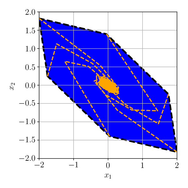
The obtained RCI sets are depicted in Fig. 2. It can be observed that the proposed direct data-driven approach is able to generate RCI sets which are of comparable volume to those obtained with the model-based method. The main advantage is that explicit knowledge of model matrices is not required, thus avoiding an additional identification step. The corresponding volumes of the RCI sets are reported in Table I, which shows that iterative Algorithm 2 with dilated LMI conditions generates relatively larger size RCI sets than those computed with the one-step Algorithm 1, which indicate that Algorithm 2 is indeed less conservative for this example.
Furthermore, Fig. 2 also shows closed-loop state trajectories starting from each vertex of the RCI set. These trajectories are obtained by simulating the true system in closed-loop with the state-feedback controller . During the closed-loop simulation, a random disturbance uniformly distributed in the interval is acting on the system at each time instance. The figure shows that the approach guarantees robust invariance in the presence of a bounded but unknown disturbance while respecting the state-constraints. The corresponding input trajectories computed with the iterative data-driven algorithm are shown in Fig. 3. The figure shows that the input constraints are also satisfied.
VI-2 RCI sets with different complexities
In this subsection, we analyse the effect of choosing different matrices corresponding to different complexities of polytope. The RCI set and the associated state-feedback gain matrices are computed running Algorithm 1 and the computed matrices are as follows,


| Complexity | |||
|---|---|---|---|
| Volume of | 4.19 | 7.04 | 8.29 |
The subscripts in (VI-2) indicate the set complexity . In Fig. 4 maximum volume RCI set with complexities are plotted along with the closed-loop state trajectories obtained by simulating the true system from different initial conditions and randomly varying the disturbance within the chosen bounds. The corresponding volume of the RCI sets are reported in Table II.
As expected, it can be observed that as increases, size of the RCI set increases, thus can be used as an additional tuning parameter to obtain an invariant set with larger volume.
VII CONCLUSIONS
We proposed a direct data-driven approach to compute a full complexity polytopic RCI set and an associated linear state-feedback control law. In the proposed algorithm neither the model of the system is required to be known nor any identification step is necessary. The algorithm is robust w.r.t. a set of all feasible models compatible with the available state-input data and satisfying the disturbance bounds. The proposed direct data-driven approach is able to generate RCI sets with sizes that are comparable to that of an approach in which exact system knowledge is assumed. As a future work, the proposed approach can be extended to generate RCI sets and controllers for a more general class of systems, e.g., linear parameter-varying and non-linear systems.
References
- [1] K. M. Abadir and J. R. Magnus. Matrix Algebra. Econometric Exercises. Cambridge University Press, 2005.
- [2] J. Berberich, A. Koch, C. W. Scherer, and F. Allgöwer. Robust data-driven state-feedback design. In Proc. of the 2020 American Control Conference (ACC), pages 1532–1538, Denver, CO, USA, 2020.
- [3] J. Berberich, C. W. Scherer, and F. Allgöwer. Combining prior knowledge and data for robust controller design. IEEE Transactions on Automatic Control, pages 1–16, 2022.
- [4] A. Bisoffi, C. De Persis, and P. Tesi. Data-based guarantees of set invariance properties. In Proc. of the 21st IFAC World Congress, pages 3953–3958, Berlin, Germany, 2020.
- [5] A. Bisoffi, C. De Persis, and P. Tesi. Controller design for robust invariance from noisy data. IEEE Transactions on Automatic Control, 68(1):636–643, 2023.
- [6] F. Blanchini. Set invariance in control. Automatica, 35(11):1747–1767, 1999.
- [7] F. Blanchini and S. Miani. Set-Theoretic Methods in Control. Birkhäuser, Boston, MA, 2015.
- [8] T. B. Blanco, M. Cannon, and B. De Moor. On efficient computation of low-complexity controlled invariant sets for uncertain linear systems. International Journal of Control, 83(7):1339–1346, July 2010.
- [9] Y. Chen and N. Ozay. Data-driven computation of robust control invariant sets with concurrent model selection. IEEE Transactions on Control Systems Technology, 30(2):495–506, 2022.
- [10] C. De Persis and P. Tesi. Formulas for data-driven control: Stabilization, optimality, and robustness. IEEE Transactions on Automatic Control, 65(3):909–924, 2020.
- [11] S. Diamond and S. Boyd. CVXPY: A Python-embedded modeling language for convex optimization. Journal of Machine Learning Research, 17(83):1–5, 2016.
- [12] M. Fiacchini, T. Alamo, and E.F. Camacho. On the computation of convex robust control invariant sets for nonlinear systems. Automatica, 46(8):1334–1338, 2010.
- [13] A. Gupta and P. Falcone. Full-complexity characterization of control-invariant domains for systems with uncertain parameter dependence. IEEE Control System Letter, 3(1):19–24, 2019.
- [14] A. Gupta, H. Köroğlu, and P. Falcone. Restricted-complexity characterization of control-invariant domains with application to lateral vehicle dynamics control. Conference on Decision and Control, pages 4956–4951, 2017.
- [15] A. Gupta, H. Köroğlu, and P. Falcone. Computation of robust control invariant sets with predefined complexity for uncertain systems. International Journal of Robust and Nonlinear Control, 31(5):1674–1688, 2021.
- [16] A. Gupta, M. Mejari, P. Falcone, and D. Piga. Computation of parameter dependent robust invariant sets for LPV models with guaranteed performance. Automatica, 151:110920, 2023.
- [17] Z. S. Hou and Z. Wang. From model-based control to data-driven control: Survey, classification and perspective. Information Sciences, 235:3–35, 2013.
- [18] C. Liu and I. M. Jaimoukha. The computation of full-complexity polytopic robust control invariant sets. In Proc. of the 54th IEEE Conf. on Decision and Control, pages 6233–6238, Osaka, Japan, 2015.
- [19] MOSEK. Mosek aps fusion api for python 10.0.40- academic license. https://docs.mosek.com/latest/pythonapi/index.html, 2023.
- [20] S. Mulagaleti, A. Bemporad, and M. Zanon. Data-driven synthesis of robust invariant sets and controllers. IEEE Control Systems Letters, 6:1676–1681, 2022.
- [21] S. V. Raković and M. Baric. Parameterized Robust Control Invariant Sets for Linear Systems: Theoretical Advances and Computational Remarks. IEEE Transactions on Automatic Control, 55(7):1599–1614, Jul 2010.
- [22] C. W. Scherer. A full block S-procedure with applications. In Proc. of the 36th IEEE Conference on Decision and Control, volume 3, pages 2602–2607, San Diego, CA, USA, 1997.
- [23] F. Tahir and I. M. Jaimoukha. Low-complexity polytopic invariant sets for linear systems subject to norm-bounded uncertainty. IEEE Transactions on Automatic Control, 60(5):1416–1421, 2015.
- [24] B. Zhong, M. Zamani, and M. Caccamo. Synthesizing safety controllers for uncertain linear systems: A direct data-driven approach. In Proc. of the Conference on Control Technology and Applications (CCTA), pages 1278–1284, Trieste, Italy, 2022.