Scale-Invariant Model for Gravitational Waves and Dark Matter

Maciej Kierkla Bogumiła Świeżewska Affiliation: Faculty of Physics, University of Warsaw, Pasteura 5, 02-093 Warsaw, Poland; Email: maciej.kierkla@fuw.edu.pl Email: bogumila.swiezewska@fuw.edu.pl Affiliation: E-mail: ;

Abstract:

The present contribution summarises the results recently published in Ref. [1]. We have conducted a revised analysis of the first-order phase transition that is associated with symmetry breaking in a classically scale-invariant model that has been extended with a new $SU(2)$ gauge group. By incorporating recent developments in the understanding of supercooled phase transitions, we were able to calculate all of its features and significantly limit the parameter space. We were also able to predict the gravitational wave spectra generated during this phase transition and found that this model is well-testable with LISA. Additionally, we have made predictions regarding the relic dark matter abundance. Our predictions are consistent with observations but only within a narrow part of the parameter space. We have placed significant constraints on the supercool dark matter scenario by improving the description of percolation and reheating after the phase transition, as well as including the running of couplings. Finally, we have also analyzed the renormalization-scale dependence of our results.

^†^†conference: Corfu Summer Institute 2022 “School and Workshops on Elementary Particle Physics and Gravity”,
28 August - 1 October 2022,
Corfu, Greece

1 Introduction

Considering the recent direct detection of gravitational waves (GW) by the LIGO and Virgo Collaborations [2, 3, 4, 5, 6, 7], as well as the upcoming Laser Interferometer Space Antenna (LISA) [8, 9, 10, 11, 12, 13] and other future and ongoing experiments [14, 15, 16, 17, 18, 19, 20, 21, 22, 23], it is reasonable to explore ways to utilize GW to investigate fundamental physics. One promising method is to search for evidence of a first-order phase transition (PT) in the early Universe through the primordial gravitational wave background [24, 9, 11, 10, 12, 13]. This signal is expected to be present at frequencies within LISA’s sensitivity range if the transition occurred around temperatures similar to those of the electroweak PT, $T\sim 100\ \,\mathrm{GeV}$ . However, in many models, the signal is not strong enough to be detected. In contrast, the class of models with classical scale invariance [25, 26, 27, 28, 29, 30, 31, 32, 33, 34, 35, 36, 37, 38] typically predicts a strong gravitational wave signal within LISA’s reach due to a logarithmic potential that enables significant supercooling and latent heat release during the transition.

Within the wide variety of classically conformal models, those incorporating an additional gauge group are particularly promising due to their high level of predictability. The conformal Standard Model (SM) can be extended in a minimal manner with the addition of either an extra $U(1)$ [39, 40, 41, 42, 43, 44, 45, 46, 47, 48, 49, 50, 51, 52, 53, 54, 55, 56, 57, 58, 59, 60, 61, 28, 62, 63, 64, 65, 33, 66, 67, 34, 36, 68, 69, 70, 37, 38] or $SU(2)$ [25, 71, 50, 72, 73, 74, 75, 64, 31, 32, 76] symmetry, and there are other possibilities such as models featuring an extended scalar sector [40, 77, 78, 79, 80, 81, 82, 83, 84, 85, 86, 87, 88, 89, 50, 90, 91, 92, 93, 94, 95, 96, 97, 98, 99, 100, 101, 102, 103, 104, 105, 29, 30, 106, 107, 108, 109, 110, 111, 112, 113, 114, 115, 116, 117, 118], larger gauge groups, extra fermions, or more intricate architectures [119, 120, 121, 122, 123, 124, 125, 126, 127, 128, 129, 130, 131, 132, 133, 134, 135, 136, 137, 138]. The focus of our current work is on the first-order PT in a classically scale-invariant model that includes an additional $SU(2)_{X}$ gauge symmetry and a scalar that transforms as a doublet under this group while remaining a singlet of the SM. In addition to exhibiting a strong first-order phase transition, this model also provides a candidate for dark matter particles that are stabilized by a residual symmetry that persists after the $SU(2)_{X}$ symmetry is broken [139, 140].

Although the possibility of detecting GW from a PT and exploring events that occurred in the early Universe is exciting, the imprecise nature of theoretical predictions is discouraging [141, 142]. The dependence on the renormalisation scale is one of the main sources of uncertainty in these predictions. Classically scale-invariant models, owing to the logarithmic nature of their potential, span a broad range of energies and therefore are particularly susceptible to issues related to scale dependence. In this work [1]:

1.

We present updated predictions of the stochastic GW background in the classically scale-invariant model with $SU(2)_{X}$ symmetry, incorporating recent advances in understanding supercooled PTs [143, 144, 145, 146, 147]. Our study is the first to include the condition for percolation in the SU(2)_X model, and we show that it significantly affects the parameter space.
2.

We pay close attention to the renormalisation-scale dependence of the results. To minimise this dependence, we use a renormalisation-group improved effective potential and perform an expansion in powers of couplings consistent with the conditions from conformal symmetry breaking and the radiative nature of the transition.
3.

We investigate the DM phenomenology in light of the updated understanding of the PT.

2 The model

In this work [1], we analyse the classically scale-invariant SM extended by a dark $SU(2)_{X}$ gauge group. The new fields of the model are:

•

the scalar doublet $\Phi$ of $SU(2)_{X}$ ,
•

the three dark gauge bosons $X$ of $SU(2)_{X}$ .

The Higgs $H$ and new scalar $\Phi$ doublets can be written as

H=\frac{1}{\sqrt{2}}\left(\begin{array}[]{c}0\\ h\end{array}\right),\quad\Phi=\frac{1}{\sqrt{2}}\left(\begin{array}[]{c}0\\ \varphi\end{array}\right)\,.

In terms of $h$ and $\varphi$ , the one-loop effective potential can be written as

V(h,\varphi)=V^{(0)}(h,\varphi)+V^{(1)}(h,\varphi),

(1)

where the tree-level part is

V^{(0)}(h,\varphi)=\frac{1}{4}\left(\lambda_{1}h^{4}+\lambda_{2}h^{2}\varphi^{2}+\lambda_{3}\varphi^{4}\right)\,,

(2)

with $\lambda_{2}$ being the portal coupling that connects the visible and dark sectors. The one-loop correction is given by

V^{(1)}(h,\varphi)=\frac{1}{64\pi^{2}}\sum_{a}n_{a}M_{a}^{4}(h,\varphi)\left(\log\frac{M_{a}^{2}(h,\varphi)}{\mu^{2}}-C_{a}\right),

(3)

where

n_{a}=(-1)^{2s_{a}}Q_{a}N_{a}(2s_{a}+1),

and the sum runs over all particle species. With $M_{a}(h,\varphi)$ we denote the field-dependent mass of a particle, $n_{a}$ denotes the number of degrees of freedom associated with each species and $C_{a}=\frac{5}{6}$ for vector bosons and $C_{a}=\frac{3}{2}$ for other particles. Furthermore, $Q_{a}=1$ for uncharged particles, and $Q_{a}=2$ for charged particles, $N_{a}=1,\,3$ for uncoloured and coloured particles, respectively.

Regarding symmetry breaking, the stationary point equations divided by the VEVs, $v=\langle h\rangle$ , $w=\langle\varphi\rangle$ , read

	$\displaystyle\frac{1}{v^{3}}\frac{\partial V}{\partial h}=\lambda_{1}$	$\displaystyle+\frac{1}{2}\lambda_{2}\left(\frac{w}{v}\right)^{2}+\frac{1}{v^{3}}\left.\frac{\partial V^{(1)}}{\partial h}\right\|_{h=v,\varphi=w}=0,$		(4)
	$\displaystyle\frac{1}{w^{3}}\frac{\partial V}{\partial\varphi}=\lambda_{3}$	$\displaystyle+\frac{1}{2}\lambda_{2}\left(\frac{v}{w}\right)^{2}+\frac{1}{w^{3}}\left.\frac{\partial V^{(1)}}{\partial\varphi}\right\|_{h=v,\varphi=w}=0.$		(5)

Typically, $v_{\varphi}/v_{h}\gg 10$ , therefore the $\lambda_{2}\left(v_{h}/v_{\varphi}\right)^{2}$ term can be neglected. Then, the second equation becomes

\lambda_{3}=-\frac{9}{256\pi^{2}}g_{X}^{4}\left[2\log\left(\frac{g_{X}}{2}\frac{w}{\mu}\right)-\frac{1}{3}\right].

(6)

The first equation reads

\lambda_{1}+\frac{1}{2}\lambda_{2}\left(\frac{w}{v}\right)^{2}+\frac{1}{16\pi^{2}}\sum_{W^{\pm},Z,t}n_{a}\frac{M_{a}^{4}(h,\varphi)}{v^{4}}\left(\log\frac{M_{a}^{2}(h,\varphi)}{\mu^{2}}-C_{a}+\frac{1}{2}\right)=0.

(7)

The above indicates that the symmetry breaking in the $\varphi$ direction follows the Coleman-Weinberg mechanism, while the symmetry breaking in the direction of $h$ is similar to that of the SM, as the ”tree-level mass term” is generated by the portal coupling.

The physical mass corresponds to a pole of the propagator, i.e. is evaluated away from $p^{2}=0$ , and is given by

M^{2}_{\mathrm{pole}}=m^{2}_{\textrm{tree-level}}+\real[\Sigma(p^{2}=M^{2}_{\mathrm{pole}})].

(8)

Including loop corrections from self energies which introduce momentum dependence, we have

M^{2}(p)=\left(\begin{array}[]{cc}3\lambda_{1}v^{2}+\frac{\lambda_{2}}{2}w^{2}&\lambda_{2}vw\\ \lambda_{2}vw&3\lambda_{3}w^{2}+\frac{\lambda_{2}}{2}v^{2}\\ \end{array}\right)+\left(\begin{array}[]{cc}\Sigma_{hh}(p)&\Sigma_{h\varphi}(p)\\ \Sigma_{h\varphi}(p)&\Sigma_{\varphi\varphi}(p)\\ \end{array}\right).

(9)

By diagonalising the mass matrix we obtain the mass eigenvalues

	$\displaystyle M^{2}_{\pm}(p^{2})$	$\displaystyle=\frac{1}{2}\Biggl\{\left(3\lambda_{1}+\frac{\lambda_{2}}{2}\right)v^{2}+\frac{1}{2}\left(\frac{\lambda_{2}}{2}+3\lambda_{3}\right)w^{2}+\Sigma_{hh}(p^{2})+\Sigma_{\varphi\varphi}(p^{2})$
		$\displaystyle\ \ \ \pm\sqrt{\left[\left(3\lambda_{1}-\frac{\lambda_{2}}{2}\right)v^{2}-\left(3\lambda_{3}-\frac{\lambda_{2}}{2}\right)w^{2}+\Sigma_{hh}(p^{2})-\Sigma_{\varphi\varphi}(p^{2})\right]^{2}+4\lambda_{2}^{2}v^{2}w^{2}}\,\Biggr\}.$		(10)

Neglecting terms suppressed by a product of a small coupling, $\lambda_{2}$ or $\lambda_{3}$ and the Higgs VEV, we can approximately determine which of the mass eigenvalues corresponds to the Higgs particle. We find

		$\displaystyle M_{+}^{2}(h,\varphi)=3\lambda_{3}\varphi^{2}+\Sigma_{\varphi\varphi}(p^{2}),$		(11)
		$\displaystyle M_{-}^{2}(h,\varphi)=3\lambda_{1}h^{2}+\frac{1}{2}\lambda_{2}\varphi^{2}+\Sigma_{hh}(p^{2})\,.$		(12)

for $3\lambda_{1}h^{2}-3\lambda_{3}\varphi^{2}+\frac{1}{2}\lambda_{2}\varphi^{2}+\Sigma_{hh}(p^{2})-\Sigma_{\varphi\varphi}(p^{2})<0$ . For the opposite sign, $M_{+}$ and $M_{-}$ are interchanged. Then, to obtain the momentum-corrected masses we solve the gap equations

	$\displaystyle M_{H}^{2}$	$\displaystyle=M_{\mp}^{2}(p^{2}=M_{H}^{2}),$		(13)
	$\displaystyle M_{S}^{2}$	$\displaystyle=M_{\pm}^{2}(p^{2}=M_{S}^{2}).$		(14)

We identify the first one with the Higgs $M_{H}=125\,\mathrm{GeV}$ , while the other gives the mass of the new scalar $S$ . Finally, the mass eigenstates are obtained from the gauge eigenstates by a rotation matrix as

\left(\begin{array}[]{c}\phi_{-}\\ \phi_{+}\end{array}\right)=\left(\begin{array}[]{rl}\cos\theta&\sin\theta\\ -\sin\theta&\cos\theta\end{array}\right)\left(\begin{array}[]{c}h\\ \varphi\end{array}\right)\,,\qquad-\frac{\pi}{2}<\theta<\frac{\pi}{2}\,.

(15)

In order to scan the parameter space, we employ the following numerical procedure:

1.

We choose the values of the input parameters, $M_{X}$ and $g_{X}$ . We assume the tree-level relation for the $X$ mass $M_{X}=\frac{1}{2}g_{X}v_{\varphi}$ so we can compute the value of the $\varphi$ VEV, $v_{\varphi}$ . The values of $g_{X}$ and $v_{\varphi}$ are treated as evaluated at the scale $\mu=M_{X}$ .
2.

We use the minimisation condition along the $\varphi$ direction, evaluated at $\mu=M_{X}$ to evaluate $\lambda_{3}$ . This gives us a simple relation

$\lambda_{3}=\frac{3}{256\pi^{2}}g_{X}^{4}.$
3.

The $g_{X}$ and $\lambda_{3}$ couplings are evolved using their RGEs and evaluated at $\mu=M_{Z}$ .
4.

If $g_{X}(M_{Z})\leqslant 1.15$ the RG-improved potential is well-behaved throughout the scales considered.
5.

The value of $\lambda_{2}$ as a function of $\lambda_{1}(\mu=M_{Z})$ is obtained from the first minimisation condition.
6.

The value of $\lambda_{1}$ is computed from the requirement that the physical Higgs mass is equal to $125\ \rm{GeV}$ , using the first gap equation. The evaluation is performed at $\mu=M_{Z}$ , therefore the vacuum expectation value of $\varphi$ at $\mu=M_{Z}$ is needed. It is found using the second minimisation condition evaluated at $\mu=M_{Z}$ .
7.

The mass of $S$ is computed by solving iteratively the second gap equation.
8.

The mixing between the scalars is evaluated by demanding that the off-diagonal terms of the mass matrix evaluated at $p^{2}=0$ and in the mass-eigenbasis are zero.

Refer to caption — Figure 1: Values of the new scalar mass $M_{S}$ (left panel) and the VEV $w$ (evaluated at $\mu=M_{X}$ ) (right panel). In the left panel the thick black line indicates where $M_{S}=M_{H}=125\,\mathrm{GeV}$ and across this line mass ordering between $S$ and $H$ changes (to the left of the line $M_{S}<M_{H}$ , and to the right $M_{H}<M_{S}$ ). To the right of the dotted line $\xi_{H}$ becomes numerically equal to 1. The dashed lines indicate a discrepancy between the running and the pole mass (in percent). Grey-shaded regions are excluded.

We present the result of the scan for $M_{S}$ and $w$ (the VEV of $\varphi$ ) in figure 1. The new scalar $S$ is heavier than the Higgs boson in most of the parameter space. The dashed lines in the plot represent the disparity between the mass obtained by solving eq. (14) iteratively and the mass estimated from the effective potential approximation. Although the differences are not negligible, they do not exceed 10% even in the upper right region of the parameter space. Finally, the region of low $X$ masses is excluded because it is not possible the reproduce a stable minimum with the correct Higgs VEV and mass in this regime, while the upper right corner is cut off by the condition $g_{X}(M_{Z})\leq 1.15$ for the perturbativity of the dark gauge coupling.

3 Dark matter

Our DM candidates are the three vector bosons $X_{\mu}^{a}$ (where $a=1,\,2,\,3$ ) of the hidden sector gauge group $SU(2)$ with mass $M_{X}=\frac{1}{2}g_{X}w$ . As discussed in [139], the gauge bosons are stable due to an intrinsic $\mathbb{Z}_{2}\crossproduct\mathbb{Z}_{2}^{\prime}$ symmetry associated with complex conjugation of the group elements and discrete gauge transformations. This discrete symmetry actually generalizes to a custodial $SO(3)$ [140] and the dark gauge bosons are degenerate in mass.

For the standard freeze-out mechanism, the Boltzmann equation has the form

\frac{\differential n}{\differential t}+3\,H\,n=-\,\frac{\left<\sigma v\right>_{\rm ann}}{3}\left(n^{2}-n^{2}_{eq}\right)-\frac{2\left<\sigma v\right>_{\rm semi}}{3}\,n\left(n-n_{eq}\right)\,.

(16)

The annihilation cross section is dominated by the $XX\rightarrow SS$ process

\left<\sigma v\right>_{\rm ann}=\frac{11g_{X}^{4}}{2304\pi M^{2}_{X}}\,,

(17)

while the semiannihilation cross section is dominated by the $XX\rightarrow XS$ process

\left<\sigma v\right>_{\rm semi}=\frac{3g_{X}^{4}}{128\pi M_{X}^{2}}\,.

(18)

Interestingly, the semiannihilation processes dominate since $\left<\sigma v\right>_{\rm semi}\sim 5\left<\sigma v\right>_{\rm ann}$ .

Solving the Boltzmann equation, we obtain the dark matter relic abundance

\Omega_{X}h^{2}=\frac{1.04\times 10^{9}\,\,{\rm GeV}^{-1}}{\sqrt{g_{*}}\,M_{P}\,J(x_{f})},\qquad J(x_{f})=\int_{x_{f}}^{\infty}dx\,\frac{\left<\sigma v\right>_{\rm ann}+2\left<\sigma v\right>_{\rm semi}}{x^{2}}\,,

(19)

where $x_{f}\approx 25-26$ and $x=M_{X}/T$ . The correct relic abundance $\Omega_{\rm DM}h^{2}=0.120\pm 0.001$ is reproduced if

g_{X}\approx 0.9\times\sqrt{\frac{M_{X}}{1\ \rm TeV}}\,.

(20)

Finally, DM particles can scatter off of nucleons, with the spin-independent cross section given by

\sigma_{\rm SI}=\frac{m_{N}^{4}f^{2}}{16\pi v^{2}}\bigg(\frac{1}{M_{S}^{2}}-\frac{1}{M_{H}^{2}}\bigg)^{2}g_{X}^{2}\sin^{2}2\alpha\simeq\frac{64\pi^{3}f^{2}m_{N}^{4}}{81M_{X}^{6}}\approx 0.6\times 10^{-45}\ \rm{cm}^{2}\left(\frac{\,{\rm TeV}}{M_{X}}\right)^{6}\,.

(21)

Then, to evade the experimental bounds we would have $\sigma_{\rm SI}<1.5\times 10^{-45}\ \rm{cm}^{2}\,\left(M_{X}/\,{\rm TeV}\right)$ for $M_{X}>0.88\,{\rm TeV}$ .

4 Finite temperature

The temperature-dependent effective potential is

V(h,\varphi,T)=V^{(0)}(h,\varphi)+V^{(1)}(h,\varphi)+V^{T}(h,\varphi,T)+V_{\textrm{daisy}}(h,\varphi,T).

(22)

The finite-temperature correction is

V^{T}(h,\varphi,T)=\frac{T^{4}}{2\pi^{2}}\sum_{a}n_{a}J_{a}\left(\frac{M_{a}(h,\varphi)^{2}}{T^{2}}\right),

(23)

where the sum runs over particle species. $J_{a}$ denotes the thermal function, which is given by

J_{F,B}(y^{2})=\int_{0}^{\infty}\differential{x}x^{2}\log(1\pm e^{-\sqrt{x^2 + y^2}}),

(24)

where “ $+$ ” for fermions ( $J_{F}$ ) and “ $-$ ” for bosons ( $J_{B}$ ). The correction from the daisy-resummed diagrams is

V_{\textrm{daisy}}(h,\varphi,T)=-\frac{T}{12\pi}\sum_{i}n_{i}\left[(M_{i,\textrm{th}}^{2}(h,\varphi,T))^{3/2}-(M_{i}^{2}(h,\varphi))^{3/2}\right],

(25)

where $n_{i}$ is the number of degrees of freedom, $M_{i,\textrm{th}}$ denotes thermally corrected mass, and $M_{i}$ the usual field dependent mass.

The zero-temperature part of the effective potential along the $\varphi$ direction reads

V(\varphi)=\frac{1}{4}\lambda_{3}(t)Z_{\varphi}(t)^{2}\varphi^{4}+\frac{9M_{X}(\varphi,t)^{4}}{64\pi^{2}}\left(\log\frac{M_{X}(\varphi,t)^{2}}{\mu^{2}}-\frac{5}{6}\right),

(26)

where $t=\log\frac{\mu}{\mu_{0}}$ , $\mu_{0}=M_{Z}$ , $M_{X}(\varphi,t)=\frac{1}{2}g_{X}(t)\sqrt{Z_{\varphi}(t)}\varphi$ , $\mu=\frac{1}{2}g_{X}(M_{X})\varphi\equiv\overline{M}_{X}(\varphi)$ .

Note that we include more terms in the renormalisation-group improved potential than in the approaches often found in the literature. In detail:

1.

The approach of [64, 31] approximates the running quartic coupling via its $\beta$ function, relates the renormalisation scale with the field and uses as a reference scale the scale at which $\lambda_{\varphi}$ changes sign,

$V_{1}\approx\frac{1}{4}\lambda_{3}(t)\varphi^{4}\approx\frac{1}{4}\frac{9g_{X}^{4}}{128\pi^{2}}\log(\frac{\f}{\f_0}),$ (27)

where $t=\log\frac{\mu}{\varphi_{0}}$ , $\lambda_{\varphi}(0)=0$ and $g_{X}$ is evaluated at $\mu=\varphi_{0}$ (the running of $g_{X}$ is not included).
2.

The approach of [147] also approximates the one-loop potential by the tree-level potential with running coupling but uses $\mu=\varphi$ and some fixed reference scale $\mu_{0}=m_{t}$ ,

$V_{2}\approx\frac{1}{4}\lambda_{3}(t)\varphi^{4},$ (28)

where $t=\log(\frac{\f}{\mu_0})$ .

To better understand which contributions are crucial we perform a series of approximations or modifications on our approach, the results of which are presented in the right panel of figure 2. Namely:

Figure 2: Effective potential at zero temperature along the

\varphi

direction for a benchmark point with

g_{X}=0.9

M_{X}=10^{4}\,\mathrm{GeV}

(defined at

\mu=M_{X}

). Left panel: Comparison of different approaches used in the literature,

V_{1}

of eq. (27) (yellow solid),

V_{2}

of eq. (28) (dashed red) and the full potential

V

of eq. (26) used in this work (solid blue). Right panel: Comparison of different approximations imposed on the full potential

V

of eq. (26) used in this work (solid blue) discussed in the main text:

V_{b}

(long-dashed darkest green),

V_{c}

(medium-dashed dark green),

V_{d}

(short-dashed light green).

1.

$V_{a}$ corresponds to the potential $V$ with the part proportional to the logarithm neglected. $V_{a}$ exactly overlaps with the full potential (solid blue line).
2.

$V_{b}$ corresponds to the potential $V$ with the choice of $\mu=\varphi$ (darkest green, long-dashed line). This choice alone does not modify the potential significantly with respect to our choice (solid blue line).
3.

$V_{c}$ corresponds to the potential $V$ with the constant $-\frac{5}{6}$ neglected (dark green, medium-dashed curve). Since the omission of the logarithm (with our choice of the scale) does not visibly modify the result, $V_{c}$ is equivalent to using the tree-level part of $V$ . Here the difference with respect to the full potential is significant. It is understandable, since the choice of the scale was such as to get rid of the logarithmic term but not the $\frac{5}{6}$ constant.
4.

$V_{d}$ corresponds to the tree-level part of $V$ but with the choice $\mu=\varphi$ (light green, short-dashed line), which makes this choice very close to $V_{1}$ and $V_{2}$ discussed above. Clearly, $V_{d}$ differs significantly from the full potential.

5 Phase transition and gravitational wave signal

A first-order phase transition proceeds through nucleation, growth and percolation of bubbles filled with the broken-symmetry phase in the sea of the symmetric phase. This corresponds to the fields tunnelling through a potential barrier. In our case, we have checked that tunnelling proceeds along the $\varphi$ direction, while the transition in the $h$ direction is smooth.

5.1 Important temperatures

The temperatures relevant to our discussion are:

Critical Temperature $T_{c}$ .

At high temperatures the symmetry is restored and the effective potential has a single minimum at the origin of the field space. As the Universe cools down, a second minimum is formed. At the critical temperature, the two minima are degenerate, and for lower temperatures, the minimum with broken symmetry becomes the true vacuum. This is the temperature at which the tunnelling becomes possible.

Thermal Inflation Temperature $T_{V}$ .

If there is large supercooling, i.e. the phase transition is delayed to low temperatures, much below the critical temperature, it is possible that a period of thermal inflation due to the false vacuum energy appears before the phase transition completes. The Hubble parameter can be written as

H^{2}=\frac{1}{3\bar{M}_{\rm{Pl}}^{2}}(\rho_{R}+\rho_{V})=\frac{1}{3\bar{M}_{\rm{Pl}}^{2}}\left(\frac{T^{4}}{\xi^{2}_{g}}+\Delta V\right),\quad\xi_{g}=\sqrt{30/(\pi^{2}g_{*})}\,,

(29)

where $\Delta V$ is the difference between the values of the effective potential at false and true vacuum. The onset of the period of thermal inflation can be approximately attributed to the temperature at which vacuum and radiation contribute to the energy density equally,

T_{V}\equiv\left(\xi^{2}_{g}\Delta V\right)^{\frac{1}{4}}.

(30)

For supercooled transitions, it is a good approximation to assume that $\Delta V$ is independent of the temperature below $T_{V}$ . By using the temperature $T_{V}$ , the Hubble constant can be rewritten as

H^{2}\simeq\frac{1}{3\bar{M}_{\rm{Pl}}^{2}\xi^{2}_{g}}\left(T^{4}+T_{V}^{4}\right).

(31)

In the case of large supercooling, the contribution to the Hubble parameter from radiation energy can be neglected, leaving

H^{2}\simeq H^{2}_{V}=\frac{1}{3\bar{M}_{\rm{Pl}}^{2}}\Delta V.

(32)

In figure 3 there are the same excluded areas as before and two new shaded regions. The lower left corner (darkest grey) is not analysed because there the PT is sourced by the QCD phase transition, which is beyond the scope of the present work. The light-grey region around $M_{X}\approx 10^{6}\,\mathrm{GeV}$ is where the percolation criterion of eq. (42) is violated and is discussed in more detail below.

Nucleation Temperature $T_{n}$ .

Below the critical temperature, nucleation of bubbles of true vacuum becomes possible. To compute the decay rate of the false vacuum we start by solving the bounce equation,

\frac{\differential^{2}\varphi}{\differential r^{2}}+\frac{2}{r}\frac{\differential\varphi}{\differential r}=\frac{\differential V(\varphi,T)}{\differential\varphi},\qquad\frac{\differential\varphi}{\differential r}=0\quad\text{ for }\quad r=0\quad\text{ and }\quad\varphi\to 0\quad\text{ for }\quad r\to\infty.

(33)

Once the bubble profile is known we can compute the Euclidean action along the tunnelling path

S_{3}(T)=4\pi\int r^{2}\mathrm{d}r\frac{1}{2}\left(\frac{\mathrm{d}\varphi}{\mathrm{d}r}\right)^{2}+V(\varphi,T).

(34)

Then the decay rate of the false vacuum due to the thermal fluctuations is given by

\Gamma(T)\approx T^{4}\left(\frac{S_{3}(T)}{2\pi T}\right)^{3/2}e^{-S_{3}(T)/T}.

(35)

The nucleation temperature is defined as the temperature at which at least one bubble is nucleated per Hubble volume, which can be interpreted as the onset of the PT.

N(T_{n})=1=\int_{t_{c}}^{t_{n}}dt\frac{\Gamma(t)}{H(t)^{3}}=\int_{T_{n}}^{T_{c}}\frac{dT}{T}\frac{\Gamma(T)}{H(T)^{4}}.

(36)

The common criterion for evaluating $T_{n}$ as $S_{3}/T_{n}\approx 140$ is not reliable in the case of strongly supercooled transitions.

Percolation Temperature $T_{p}$ .

When the bubbles of the true vacuum percolate, most of the bubble collisions take place. Therefore, the percolation temperature is the relevant temperature for the GW signal generation. The probability of finding a point still in the false vacuum at a certain temperature is given by $P(T)=e^{-I(T)}$ , where $I(T)$ is the amount of true vacuum volume per unit comoving volume and reads as

I(T)=\frac{4\pi}{3}\int_{T}^{T_{c}}\differential{T^\prime}\frac{\Gamma(T^{\prime})}{T^{\prime 4}H(T^{\prime})}\left(\int_{T}^{T^{\prime}}\frac{\differential{\tilde T}}{H(\tilde{T})}\right)^{3}.

(37)

We can distinguish between the vacuum and radiation domination period which leads to the Hubble parameter in the following form:

\displaystyle H(T)\simeq\left\{\begin{array}[]{ll}H_{\mathrm{R}}(T)=\frac{T^{2}}{\sqrt{3}\bar{M}_{\mathrm{pl}}\xi_{g}},&\quad\mathrm{for}\quad T>T_{V},\\ H_{\mathrm{V}}=\frac{T_{V}^{2}}{\sqrt{3}\bar{M}_{\mathrm{pl}}\xi_{g}},&\quad\mathrm{for}\quad T<T_{V}.\end{array}\right.

We can thus write a simplified version of $I(T)$ valid in the region where $T<T_{V}$ :

\displaystyle\begin{split}I_{\mathrm{RV}}(T)=\frac{4\pi}{3H_{\mathrm{V}}^{4}}\left(\int_{T_{V}}^{T_{c}}\frac{dT^{\prime}\Gamma\left(T^{\prime}\right)}{T^{\prime 6}}T_{V}^{2}\left(2T_{V}-T-\frac{T_{V}^{2}}{T^{\prime}}\right)^{3}+\int_{T}^{T_{V}}\frac{dT^{\prime}\Gamma\left(T^{\prime}\right)}{T^{\prime}}\left(1-\frac{T}{T^{\prime}}\right)^{3}\right)\end{split}

(40)

The percolation criterion is given by

I_{\mathrm{RV}}(T_{p})=0.34\,,\qquad\text{or}\qquad P(T_{p})=0.7\,.

(41)

The fraction 0.34 is the ratio of the volume in equal-size and randomly-distributed spheres (including overlapping regions) to the total volume of space for which percolation occurs in three-dimensional Euclidean space, and implies that at $T_{p}$ at least 34% of the (comoving) volume is converted to the true minimum.

Comparing to the values of $T_{n}$ (fig. 4) one can see that these two temperatures are of the same order, yet they differ, hence one should not use $T_{n}$ as a proxy for the temperature at which the PT proceeds in case of the models with large supercooling.

One also needs to make sure that the volume of the false vacuum $V_{f}\sim a^{3}(T)P(T)$ is decreasing around the percolation temperature. This condition is especially constraining in models featuring strong supercooling, as thermal inflation can prevent bubbles from percolating. It can be expressed as

\displaystyle\frac{1}{V_{f}}\frac{\differential V_{f}}{\differential t}=3H(t)-\frac{\differential I(t)}{\differential t}=H(T)\left(3+T\frac{\differential I(T)}{\differential T}\right)<0.

(42)

Reheating Temperature $T_{r}$ .

At the end of the phase transition, the Universe is in a vacuum-dominated state. Then the total energy released in the phase transition is $\Delta V(T_{p})\approx\Delta V(T=0)\equiv\Delta V$ . If reheating is instantaneous, this whole energy is turned into the energy of radiation,

\Delta V=\rho_{R}(T_{r})=\rho_{R}(T_{V})\qquad\rightarrow\qquad T_{r}=T_{V}.

(43)

On the other hand, if at $T_{p}$ the rate of energy transfer from the $\varphi$ field to the plasma, $\Gamma_{\varphi}$ , is smaller than the Hubble parameter, $\Gamma_{\varphi}<H(T_{p})$ , then the energy will be stored in the scalar field oscillating about the true vacuum and redshift as matter until $\Gamma_{\varphi}$ becomes comparable to the Hubble parameter. In this case

T_{r}=T_{V}\sqrt{\frac{\Gamma_{\varphi}}{H_{*}}}.

(44)

The rate of energy transfer from $\varphi$ to the plasma reads

\displaystyle\Gamma_{\varphi}=

\displaystyle\xi_{S}^{2}(1-\xi_{S}^{2})\Gamma_{\mathrm{SM}}(S)+(1-\xi_{S}^{2})\Gamma(S\to HH),\quad\xi_{S}=\left\{\begin{array}[]{lrl}-\sin\theta&\textrm{ for }&M_{H}\leqslant M_{S}\\ \cos\theta&\textrm{ for }&M_{H}>M_{S}\end{array}\right.

where $\Gamma_{\mathrm{SM}}$ denotes a decay width computed as in the SM, i.e. with the same couplings and decay channels, but for a particle of mass $M_{S}$ . The mixing enhances the decay width twofold, first, it amplifies the coupling $SHH$ as compared to $\varphi hh$ and, moreover, it allows a contribution from the SM sector, which is especially important when the $S\to HH$ decay is kinematically forbidden.

5.2 Supercool Dark Matter?

The authors of [64, 31, 76] claim that for a wide range of parameters, there can be supercool DM. Their main assumptions are:

•

The true vacuum has zero energy, the energy in the false vacuum is $\Delta V\simeq 9m^{4}_{\chi}/(128\pi^{2})$ , which implies that supercooling starts at

$T_{V}\simeq\frac{M_{X}}{8.5}\quad\text{and}\quad H_{*}=\sqrt{\frac{3}{\pi}}\,\frac{M^{2}_{X}}{4M_{\rm pl}}\,.$
•

Nucleation occurs when $S_{3}(T_{n})/T_{n}\simeq 4\ln(M_{\rm pl}/m_\chi)\simeq 142$ .
•

The reheating temperature is related to the thermal inflation temperature as
$T_{\rm r}=T_{V}\ \min\left(1,\Gamma/H\right)^{1/2}$ , where $\Gamma\simeq\Gamma_{h}\sin^{2}(v/w)$ , with $\Gamma_{h}\approx 4\ \rm{MeV}\,.$

•

The DM abundance resulting from inflationary supercooling is

Y_{\rm DM}\equiv\frac{n_{\rm DM}|_{T=T_{\rm r}}}{s|_{T=T_{\rm r}}}=\frac{45g_{\rm DM}}{2\pi^{4}g_{*}}\frac{T_{\rm r}}{T_{\rm V}}\left(\frac{T_{\rm n}}{T_{\rm V}}\right)^{3}\,.

•

For $T_{\rm r}<T_{\rm dec}\simeq M_{X}/25$ , both supercooling and sub-thermal production contribute to the DM relic abundance,

$\Omega_{\rm DM}h^{2}=\Omega_{\rm DM}h^{2}|_{\rm supercool}+\Omega_{\rm DM}h^{2}|_{\rm sub-thermal}\,.$
•

For $T_{\rm r}>T_{\rm dec}$ , the plasma thermalizes again, and the usual freeze-out mechanism yields the relic abundance,

$\Omega_{\rm DM}h^{2}=\Omega_{\rm DM}h^{2}|_{\rm freeze-out}\,.$

Nevertheless, our analysis suggests that due to the percolation criterion which excludes $M_{X}$ above $\sim 10^{6}\ \rm\,{\rm GeV}$ and the fact that $\Gamma_{\varphi}>H(T_{p})$ in the rest of the DM range, we find $T_{r}>T_{\rm dec}$ for all parameter points. Hence, the supercool DM population gets diluted away, the sub-thermal population reaches thermal equilibrium again, and the relic abundance is produced as in the standard freezeout scenario (see fig. 6). Our conclusions were also validated in a recent paper [152].

5.3 Gravitational waves

The GW signal in the model under consideration can be sourced by bubble collisions. The spectrum is:

\Omega_{\text{col}}(f)=\left(\frac{R_{*}H_{*}}{5}\right)^{2}\left(\frac{\kappa_{\text{col}}\alpha}{1+\alpha}\right)^{2}S_{\textrm{col}}(f)\,.

(47)

where $R_{*}$ is the length scale of the transition, $\kappa_{\text{col}}$ is the energy transfer efficiency factor at the end of the transition and $\alpha=\Delta V/\rho_{R}(T_{p})$ is the transition strength. The spectral shape $S_{\textrm{col}}$ and peak frequency are defined as

S_{\textrm{col}}=25.09\left[2.41\left(\frac{f}{f_{\textrm{col}}}\right)^{-0.56}+2.34\left(\frac{f}{f_{\textrm{col}}}\right)^{0.57}\right]^{-4.2}\,,\qquad f_{\textrm{col}}\simeq 0.13\left(\frac{5}{R_{*}H_{*}}\right).

(48)

The spectra of the sound-wave-sourced GW are expressed as:

\Omega_{\textrm{sw}}(f)=\left(\frac{R_{*}H_{*}}{5}\right)\left(1-\frac{1}{\sqrt{1+2\tau_{\textrm{sw}}H_{*}}}\right)\left(\frac{\kappa_{\text{sw}}\alpha}{1+\alpha}\right)^{2}S_{{\textrm{sw}}}(f),

(49)

with

S_{\textrm{sw}}(f)=\left(\frac{f}{f_{\textrm{sw}}}\right)^{3}\left[\frac{4}{7}+\frac{3}{7}\left(\frac{f}{f_{\textrm{sw}}}\right)^{2}\right]^{7/2}\,,

(50)

where the duration of the sound wave period normalised to Hubble and the peak frequency can be expressed as

\tau_{\textrm{sw}}H_{*}=\frac{R*H_{*}}{U_{f}},\quad U_{f}\simeq\sqrt{\frac{3}{4}\frac{\alpha}{1+\alpha}\kappa_{\textrm{sw}}}\,,\quad f_{\textrm{sw}}\simeq 0.54\left(\frac{5}{R_{*}H_{*}}\right)\,.

(51)

To assess the observability of a signal we compute the signal-to-noise (SNR) ratio for the detectors that have the best potential of observing the predicted signal, i.e. LISA and AEDGE. We calculate the SNR using the usual formula [153, 154]:

\displaystyle\mbox{SNR}=\sqrt{\mathcal{T}\int_{f_{\rm{min}}}^{f_{\rm{max}}}\differential f\left[\frac{h^{2}\Omega_{\rm{GW}}(f)}{h^{2}\Omega_{\rm{Sens}}(f)}\right]^{2}},

(52)

where $\mathcal{T}$ is the duration of collecting data and $h^{2}\Omega_{\rm{Sens}}(f)$ is the sensitivity curve of a given detector. For calculations we have used data collecting durations as $\mathcal{T}_{\rm{LISA}}$ = 75 % $\cdot$ 4 years [153] and $\mathcal{T}_{\rm{AEDGE}}$ = 3 years [17]. We will assume that a signal could be observed if $\mathrm{SNR}>10$ , which is the usual criterion.

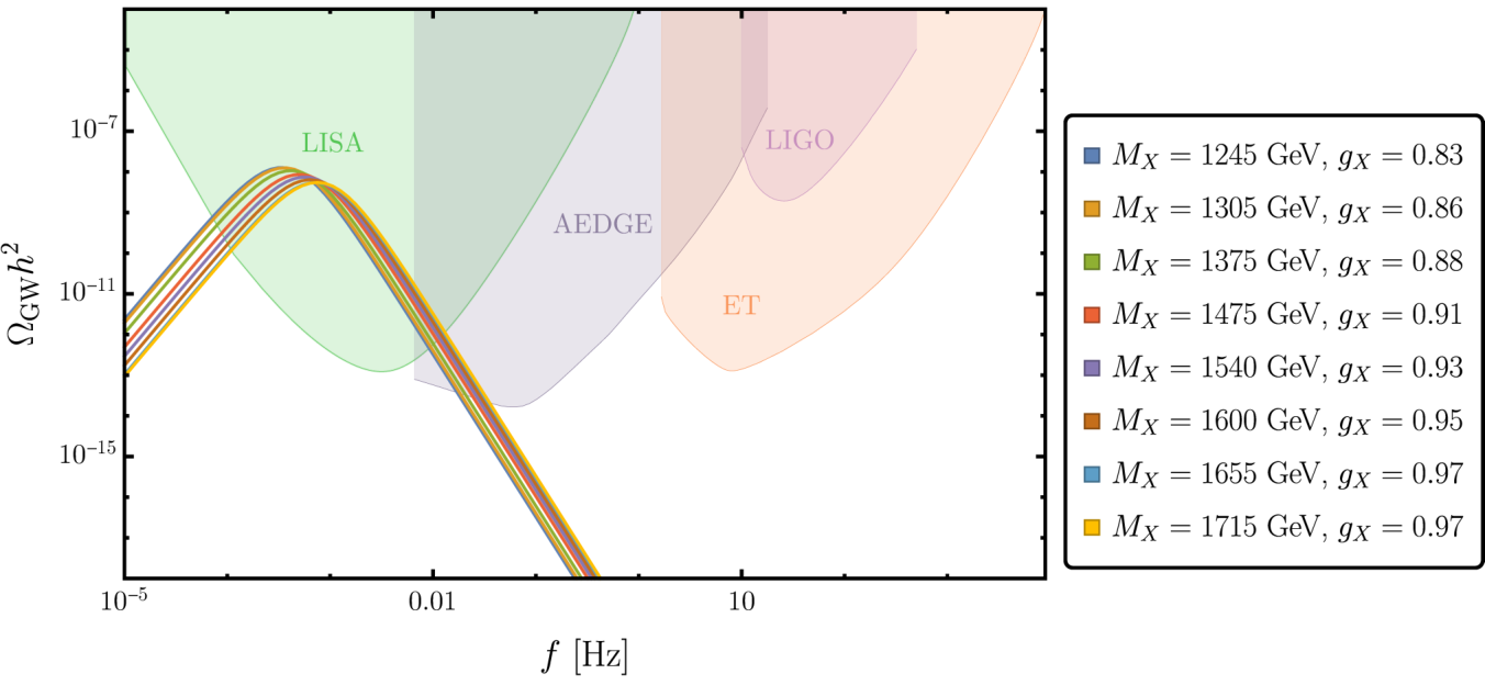
The results are presented in figure 7. Superimposed is a curve indicating where in the parameter space the correct DM relic density is reproduced and the DM direct detection constraints are satisfied (solid black). Strikingly, the SNR for LISA for the predicted signal is above the observability threshold within the whole parameter space, and almost whole in the case of AEDGE. This means that a first-order phase transition sourced by tunnelling of a scalar field in the present model should be thoroughly testable by LISA and AEDGE. Moreover, in case of not observing a signal consistent with the expectations for the first-order phase transitions this scenario could be falsified.

The correct DM relic abundance and non-exclusion by direct detection experiments (solid black line in figure 7) are located in the region of a relatively weaker signal. It is still well observable with LISA and AEDGE. The GW signal in the region where the correct abundance is reproduced is sourced entirely by sound waves. Examples of spectra for points along the black line in figure 7 are shown in figure 8.

5.4 Renormalisation-scale dependence

Finally, we perform scans of the parameter space at fixed $\mu$ . This will tell us how our understanding of the parameter space and observability of the GW signal depends on the renormalisation scale. Figure 9 shows the results for the percolation temperature $T_{p}$ computed at different scales ( $\mu=M_{X}$ (left), $\mu=M_{Z}$ (right)) together with the previous constraints on the parameter space. Both figures indicate a striking dependence on the renormalisation scale. This has further implications since for $T_{p}\lesssim 0.1\,\mathrm{GeV}$ the PT is believed to be sourced by the QCD effects, which changes the nature and properties of the PT. In this work we focus on the PT sourced by the tunnelling, therefore the considered parameter space changes dramatically as the renormalisation scale is changed. Also, the answer to a basic question – whether or not the PT completes via percolation of bubbles of the true vacuum – is altered by the change of the renormalisation scale as can be seen by examining the percolation criterion (light-grey shaded region). The results show that the change of the scale at which computations are performed not only changes the results quantitatively, by shifting the values of the characteristic parameters of the phase transition, but it also significantly modifies them qualitatively – by modifying the character of the phase transition, the very fact of its completion and the dominant source of the GW signal.

6 Summary and conclusions

In the present work, we studied a model endowed with classical scale invariance, a dark SU(2)_X gauge group and a scalar doublet of this group. This model provides a dynamical mechanism of generating all the mass scales via radiative symmetry breaking, while featuring only two free parameters. Moreover, it provides dark matter candidates – the three gauge bosons of the SU(2)_X group which are degenerate in mass – stabilised by an intrinsic $\mathbb{Z}_{2}\times\mathbb{Z}_{2}^{\prime}$ symmetry. Like other models with scaling symmetry, the studied model exhibits strong supercooling which results in the generation of an observable gravitational-wave signal.

Motivated by these attractive features we performed an analysis of the phase transition, gravitational wave generation and dark matter relic abundance, updating and extending the existing results [25, 71, 50, 72, 73, 74, 75, 64, 31, 32, 76]. The analysis features the key ingredients:

•

careful analysis of the potential in the light of radiative symmetry breaking;
•

using renormalisation-group improved potential which includes all the leading order terms;
•

using RG-running to move between various relevant scales: the electroweak scale for scalar mass generation, the scale of the mass of the new scalar for its decay during reheating;
•

careful analysis of the supercooled phase transition, following recent developments, in particular imposing the percolation criterion which proved crucial for phenomenological predictions;
•

analysis of dark matter relic abundance in the light of the updated picture of the phase transition;
•

analysis of gravitational-wave spectra using most recent results from simulations;
•

using fixed-scale potential, in addition to the renormalisation-group-improved one, to study the scale dependence of the results.

The first and foremost result of our analysis is that within the model the gravitational wave signal sourced by a first-order phase transition associated with the $SU(2)_{X}$ and electroweak symmetry breaking is strong and observable for the whole allowed parameter space. This is an important conclusion since it allows this scenario to be falsified in case of negative LISA results.

Second, we exclude the supercool dark matter scenario within the region where the phase transition proceeds via nucleation and percolation of bubbles of the true vacuum. It is a result of a combination of two reasons: we include the percolation condition, eq. (42), which allows to verify that a strongly supercooled phase transition indeed completes via percolation of bubbles and strongly constrains the parameter space relevant for our analysis. Moreover, we improve on the computation of the decay rate of the scalar field $\varphi$ , which controls the reheating rate, which pushes the onset of inefficient reheating towards higher $M_{X}$ , beyond the region of interest.

Third, we find the parameter space in which the correct relic dark matter abundance is predicted. It is produced via the standard freeze-out mechanism in the region with relatively low $M_{X}$ and large $g_{X}$ . It is the region where the phase transition is relatively weak (compared with other regions of the parameter space), yet the gravitational-wave signal should be well observable with LISA. This parameter space is further reduced due to the recent direct detection constraints.

Moreover, in the present work we focused on the issue of scale dependence of the predictions. Our approach to reducing this dependence was to implement the renormalisation-group improvement procedure, respecting the power counting of couplings to include all the relevant terms. For comparison, we present results of computations performed at fixed scale, where the dependence on the renormalisation scale is significant. It is important to note that with the change of the scale the predictions do not only change quantitatively, they can change qualitatively. For example, for computations performed at a fixed scale (both $\mu=M_{X}$ and $M_{Z}$ ) gravitational waves sourced by bubble collisions are not present. At the same time, with RG improvement we see a substantial region where bubble collisions are efficient in producing an observable signal.

To sum up, the classically scale-invariant model with an extra SU(2) symmetry remains a valid theoretical framework for describing dark matter and gravitational-wave signal produced during a first-order phase transition in the early Universe. It will be tested experimentally by LISA and other gravitational-wave detectors. The predictions, however, are sensitive to the theoretical procedures implemented. Therefore, it is crucial to improve our understanding of theoretical pitfalls affecting the predictions. The present work is a step in this direction.

Acknowledgments.

We would like to thank Kristjan Kannike, Wojciech Kotlarski, Luca Marzola, Tania Robens, Martti Raidal and Rui Santos for useful discussions. We are indebted to Marek Lewicki for numerous discussions, clarifications and sharing data for the SNR plots. We are grateful to João Viana for his computation of Higgs decay width using hdecay and IT hints. We would also like to thank Matti Heikinheimo, Tomislav Prokopec, Tommi Tenkanen, Kimmo Tuominen and Ville Vaskonen for collaboration in the early stages of this work. AK was supported by the Estonian Research Council grants MOBTT5, MOBTT86, PSG761 and by the EU through the European Regional Development Fund CoE program TK133 “The Dark Side of the Universe”. The work of BŚ and MK is supported by the National Science Centre, Poland, through the SONATA project number 2018/31/D/ST2/03302. AK would also like the thank the organizers of the “School and Workshops on Elementary Particle Physics and Gravity”, Corfu 2022, for their hospitality during his stay, and for giving him the opportunity to present this work.

References

[1] M. Kierkla, A. Karam, and B. Swiezewska, “Conformal model for gravitational waves and dark matter: a status update,” JHEP 03 (2023) 007, arXiv:2210.07075 [astro-ph.CO].
[2] Virgo, LIGO Scientific Collaboration, B. P. Abbott et al., “Observation of Gravitational Waves from a Binary Black Hole Merger,” Phys. Rev. Lett. 116 no.~6, (2016) 061102, arXiv:1602.03837 [gr-qc].
[3] Virgo, LIGO Scientific Collaboration, B. P. Abbott et al., “GW151226: Observation of Gravitational Waves from a 22-Solar-Mass Binary Black Hole Coalescence,” Phys. Rev. Lett. 116 no.~24, (2016) 241103, arXiv:1606.04855 [gr-qc].
[4] VIRGO, LIGO Scientific Collaboration, B. P. Abbott et al., “GW170104: Observation of a 50-Solar-Mass Binary Black Hole Coalescence at Redshift 0.2,” Phys. Rev. Lett. 118 no.~22, (2017) 221101, arXiv:1706.01812 [gr-qc]. [Erratum: Phys. Rev. Lett.121,no.12,129901(2018)].
[5] Virgo, LIGO Scientific Collaboration, B. Abbott et al., “GW170817: Observation of Gravitational Waves from a Binary Neutron Star Inspiral,” Phys. Rev. Lett. 119 no.~16, (2017) 161101, arXiv:1710.05832 [gr-qc].
[6] LIGO Scientific, Virgo Collaboration, B. P. Abbott et al., “GW170814: A Three-Detector Observation of Gravitational Waves from a Binary Black Hole Coalescence,” Phys. Rev. Lett. 119 no.~14, (2017) 141101, arXiv:1709.09660 [gr-qc].
[7] LIGO Scientific, Virgo Collaboration, B. . P. . Abbott et al., “GW170608: Observation of a 19-solar-mass Binary Black Hole Coalescence,” Astrophys. J. Lett. 851 (2017) L35, arXiv:1711.05578 [astro-ph.HE].
[8] N. Bartolo et al., “Science with the space-based interferometer LISA. IV: Probing inflation with gravitational waves,” JCAP 12 (2016) 026, arXiv:1610.06481 [astro-ph.CO].
[9] C. Caprini, D. G. Figueroa, R. Flauger, G. Nardini, M. Peloso, M. Pieroni, A. Ricciardone, and G. Tasinato, “Reconstructing the spectral shape of a stochastic gravitational wave background with LISA,” JCAP 11 (2019) 017, arXiv:1906.09244 [astro-ph.CO].
[10] C. Gowling and M. Hindmarsh, “Observational prospects for phase transitions at LISA: Fisher matrix analysis,” JCAP 10 (2021) 039, arXiv:2106.05984 [astro-ph.CO].
[11] LISA Cosmology Working Group Collaboration, P. Auclair et al., “Cosmology with the Laser Interferometer Space Antenna,” arXiv:2204.05434 [astro-ph.CO].
[12] G. Boileau, N. Christensen, C. Gowling, M. Hindmarsh, and R. Meyer, “Prospects for LISA to detect a gravitational-wave background from first order phase transitions,” arXiv:2209.13277 [gr-qc].
[13] C. Gowling, M. Hindmarsh, D. C. Hooper, and J. Torrado, “Reconstructing physical parameters from template gravitational wave spectra at LISA: first order phase transitions,” arXiv:2209.13551 [astro-ph.CO].
[14] L. Badurina et al., “AION: An Atom Interferometer Observatory and Network,” JCAP 05 (2020) 011, arXiv:1911.11755 [astro-ph.CO].
[15] P. W. Graham, J. M. Hogan, M. A. Kasevich, and S. Rajendran, “Resonant mode for gravitational wave detectors based on atom interferometry,” Phys. Rev. D 94 no.~10, (2016) 104022, arXiv:1606.01860 [physics.atom-ph].
[16] MAGIS Collaboration, P. W. Graham, J. M. Hogan, M. A. Kasevich, S. Rajendran, and R. W. Romani, “Mid-band gravitational wave detection with precision atomic sensors,” arXiv:1711.02225 [astro-ph.IM].
[17] AEDGE Collaboration, Y. A. El-Neaj et al., “AEDGE: Atomic Experiment for Dark Matter and Gravity Exploration in Space,” EPJ Quant. Technol. 7 (2020) 6, arXiv:1908.00802 [gr-qc].
[18] M. Punturo et al., “The Einstein Telescope: A third-generation gravitational wave observatory,” Class. Quant. Grav. 27 (2010) 194002.
[19] S. Hild et al., “Sensitivity Studies for Third-Generation Gravitational Wave Observatories,” Class. Quant. Grav. 28 (2011) 094013, arXiv:1012.0908 [gr-qc].
[20] LIGO Scientific Collaboration, G. M. Harry, “Advanced LIGO: The next generation of gravitational wave detectors,” Class. Quant. Grav. 27 (2010) 084006.
[21] VIRGO Collaboration, F. Acernese et al., “Advanced Virgo: a second-generation interferometric gravitational wave detector,” Class. Quant. Grav. 32 no.~2, (2015) 024001, arXiv:1408.3978 [gr-qc].
[22] LIGO Scientific Collaboration, J. Aasi et al., “Advanced LIGO,” Class. Quant. Grav. 32 (2015) 074001, arXiv:1411.4547 [gr-qc].
[23] LIGO Scientific, Virgo Collaboration, R. Abbott et al., “Open data from the first and second observing runs of Advanced LIGO and Advanced Virgo,” SoftwareX 13 (2021) 100658, arXiv:1912.11716 [gr-qc].
[24] C. Caprini et al., “Science with the space-based interferometer eLISA. II: Gravitational waves from cosmological phase transitions,” JCAP 1604 no.~04, (2016) 001, arXiv:1512.06239 [astro-ph.CO].
[25] T. Hambye and A. Strumia, “Dynamical generation of the weak and Dark Matter scale,” Phys. Rev. D88 (2013) 055022, arXiv:1306.2329 [hep-ph].
[26] J. Jaeckel, V. V. Khoze, and M. Spannowsky, “Hearing the signal of dark sectors with gravitational wave detectors,” Phys. Rev. D94 no.~10, (2016) 103519, arXiv:1602.03901 [hep-ph].
[27] K. Hashino, M. Kakizaki, S. Kanemura, and T. Matsui, “Synergy between measurements of gravitational waves and the triple-Higgs coupling in probing the first-order electroweak phase transition,” Phys. Rev. D94 no.~1, (2016) 015005, arXiv:1604.02069 [hep-ph].
[28] R. Jinno and M. Takimoto, “Probing a classically conformal B-L model with gravitational waves,” Phys. Rev. D95 no.~1, (2017) 015020, arXiv:1604.05035 [hep-ph].
[29] L. Marzola, A. Racioppi, and V. Vaskonen, “Phase transition and gravitational wave phenomenology of scalar conformal extensions of the Standard Model,” Eur. Phys. J. C77 no.~7, (2017) 484, arXiv:1704.01034 [hep-ph].
[30] P. H. Ghorbani, “Electroweak phase transition in the scale invariant standard model,” Phys. Rev. D 98 no.~11, (2018) 115016, arXiv:1711.11541 [hep-ph].
[31] I. Baldes and C. Garcia-Cely, “Strong gravitational radiation from a simple dark matter model,” JHEP 05 (2019) 190, arXiv:1809.01198 [hep-ph].
[32] T. Prokopec, J. Rezacek, and B. Świeżewska, “Gravitational waves from conformal symmetry breaking,” JCAP 02 (2019) 009, arXiv:1809.11129 [hep-ph].
[33] C. Marzo, L. Marzola, and V. Vaskonen, “Phase transition and vacuum stability in the classically conformal B–L model,” Eur. Phys. J. C 79 no.~7, (2019) 601, arXiv:1811.11169 [hep-ph].
[34] A. Mohamadnejad, “Gravitational waves from scale-invariant vector dark matter model: Probing below the neutrino-floor,” Eur. Phys. J. C 80 no.~3, (2020) 197, arXiv:1907.08899 [hep-ph].
[35] A. Ghoshal and A. Salvio, “Gravitational waves from fundamental axion dynamics,” JHEP 12 (2020) 049, arXiv:2007.00005 [hep-ph].
[36] Z. Kang and J. Zhu, “Scale-genesis by Dark Matter and Its Gravitational Wave Signal,” Phys. Rev. D 102 no.~5, (2020) 053011, arXiv:2003.02465 [hep-ph].
[37] A. Mohamadnejad, “Electroweak phase transition and gravitational waves in a two-component dark matter model,” JHEP 03 (2022) 188, arXiv:2111.04342 [hep-ph].
[38] A. Dasgupta, P. S. B. Dev, A. Ghoshal, and A. Mazumdar, “Gravitational Wave Pathway to Testable Leptogenesis,” arXiv:2206.07032 [hep-ph].
[39] R. Hempfling, “The Next-to-minimal Coleman-Weinberg model,” Phys. Lett. B379 (1996) 153–158, arXiv:hep-ph/9604278 [hep-ph].
[40] M. Sher, “The Coleman-Weinberg phase transition in extended Higgs models,” Phys. Rev. D 54 (1996) 7071–7074, arXiv:hep-ph/9607337.
[41] W.-F. Chang, J. N. Ng, and J. M. S. Wu, “Shadow Higgs from a scale-invariant hidden U(1)(s) model,” Phys. Rev. D75 (2007) 115016, arXiv:hep-ph/0701254 [HEP-PH].
[42] S. Iso, N. Okada, and Y. Orikasa, “Classically conformal $B-L$ extended Standard Model,” Phys. Lett. B676 (2009) 81–87, arXiv:0902.4050 [hep-ph].
[43] S. Iso and Y. Orikasa, “TeV Scale B-L model with a flat Higgs potential at the Planck scale: In view of the hierarchy problem,” PTEP 2013 (2013) 023B08, arXiv:1210.2848 [hep-ph].
[44] C. Englert, J. Jaeckel, V. V. Khoze, and M. Spannowsky, “Emergence of the Electroweak Scale through the Higgs Portal,” JHEP 04 (2013) 060, arXiv:1301.4224 [hep-ph].
[45] V. V. Khoze and G. Ro, “Leptogenesis and Neutrino Oscillations in the Classically Conformal Standard Model with the Higgs Portal,” JHEP 10 (2013) 075, arXiv:1307.3764 [hep-ph].
[46] V. V. Khoze, “Inflation and Dark Matter in the Higgs Portal of Classically Scale Invariant Standard Model,” JHEP 11 (2013) 215, arXiv:1308.6338 [hep-ph].
[47] M. Hashimoto, S. Iso, and Y. Orikasa, “Radiative symmetry breaking at the Fermi scale and flat potential at the Planck scale,” Phys. Rev. D 89 no.~1, (2014) 016019, arXiv:1310.4304 [hep-ph].
[48] M. Hashimoto, S. Iso, and Y. Orikasa, “Radiative symmetry breaking from flat potential in various U(1)’ models,” Phys. Rev. D 89 no.~5, (2014) 056010, arXiv:1401.5944 [hep-ph].
[49] S. Benic and B. Radovcic, “Electroweak breaking and Dark Matter from the common scale,” Phys. Lett. B 732 (2014) 91–94, arXiv:1401.8183 [hep-ph].
[50] V. V. Khoze, C. McCabe, and G. Ro, “Higgs vacuum stability from the dark matter portal,” JHEP 08 (2014) 026, arXiv:1403.4953 [hep-ph].
[51] S. Benic and B. Radovcic, “Majorana dark matter in a classically scale invariant model,” JHEP 01 (2015) 143, arXiv:1409.5776 [hep-ph].
[52] H. Okada and Y. Orikasa, “Classically conformal radiative neutrino model with gauged B $-$ L symmetry,” Phys. Lett. B 760 (2016) 558–564, arXiv:1412.3616 [hep-ph].
[53] J. Guo, Z. Kang, P. Ko, and Y. Orikasa, “Accidental dark matter: Case in the scale invariant local B-L model,” Phys. Rev. D91 no.~11, (2015) 115017, arXiv:1502.00508 [hep-ph].
[54] P. Humbert, M. Lindner, and J. Smirnov, “The Inverse Seesaw in Conformal Electro-Weak Symmetry Breaking and Phenomenological Consequences,” JHEP 06 (2015) 035, arXiv:1503.03066 [hep-ph].
[55] S. Oda, N. Okada, and D.-s. Takahashi, “Classically conformal U(1)’ extended standard model and Higgs vacuum stability,” Phys. Rev. D 92 no.~1, (2015) 015026, arXiv:1504.06291 [hep-ph].
[56] P. Humbert, M. Lindner, S. Patra, and J. Smirnov, “Lepton Number Violation within the Conformal Inverse Seesaw,” JHEP 09 (2015) 064, arXiv:1505.07453 [hep-ph].
[57] A. D. Plascencia, “Classical scale invariance in the inert doublet model,” JHEP 09 (2015) 026, arXiv:1507.04996 [hep-ph].
[58] N. Haba, H. Ishida, N. Okada, and Y. Yamaguchi, “Bosonic seesaw mechanism in a classically conformal extension of the Standard Model,” Phys. Lett. B 754 (2016) 349–352, arXiv:1508.06828 [hep-ph].
[59] A. Das, N. Okada, and N. Papapietro, “Electroweak vacuum stability in classically conformal B-L extension of the Standard Model,” Eur. Phys. J. C 77 no.~2, (2017) 122, arXiv:1509.01466 [hep-ph].
[60] N. Haba, H. Ishida, R. Takahashi, and Y. Yamaguchi, “Gauge coupling unification in a classically scale invariant model,” JHEP 02 (2016) 058, arXiv:1511.02107 [hep-ph].
[61] Z.-W. Wang, F. S. Sage, T. G. Steele, and R. B. Mann, “Asymptotic Safety in the Conformal Hidden Sector?,” J. Phys. G 45 no.~9, (2018) 095002, arXiv:1511.02531 [hep-ph].
[62] A. Das, S. Oda, N. Okada, and D.-s. Takahashi, “Classically conformal U(1)’ extended standard model, electroweak vacuum stability, and LHC Run-2 bounds,” Phys. Rev. D 93 no.~11, (2016) 115038, arXiv:1605.01157 [hep-ph].
[63] S. Oda, N. Okada, and D.-s. Takahashi, “Right-handed neutrino dark matter in the classically conformal U(1)’ extended standard model,” Phys. Rev. D 96 no.~9, (2017) 095032, arXiv:1704.05023 [hep-ph].
[64] T. Hambye, A. Strumia, and D. Teresi, “Super-cool Dark Matter,” JHEP 08 (2018) 188, arXiv:1805.01473 [hep-ph].
[65] F. Loebbert, J. Miczajka, and J. Plefka, “Consistent Conformal Extensions of the Standard Model,” Phys. Rev. D 99 no.~1, (2019) 015026, arXiv:1805.09727 [hep-ph].
[66] S. Yaser Ayazi and A. Mohamadnejad, “Conformal vector dark matter and strongly first-order electroweak phase transition,” JHEP 03 (2019) 181, arXiv:1901.04168 [hep-ph].
[67] Y. G. Kim, K. Y. Lee, and S.-H. Nam, “Conformal invariance and singlet fermionic dark matter,” Phys. Rev. D 100 no.~7, (2019) 075038, arXiv:1906.03390 [hep-ph].
[68] I. D. Gialamas, A. Karam, T. D. Pappas, and V. C. Spanos, “Scale-invariant quadratic gravity and inflation in the Palatini formalism,” Phys. Rev. D 104 no.~2, (2021) 023521, arXiv:2104.04550 [astro-ph.CO].
[69] B. Barman and A. Ghoshal, “Scale invariant FIMP miracle,” JCAP 03 no.~03, (2022) 003, arXiv:2109.03259 [hep-ph].
[70] B. Barman and A. Ghoshal, “Probing pre-BBN era with Scale Invariant FIMP,” arXiv:2203.13269.
[71] C. D. Carone and R. Ramos, “Classical scale-invariance, the electroweak scale and vector dark matter,” Phys. Rev. D88 (2013) 055020, arXiv:1307.8428 [hep-ph].
[72] G. M. Pelaggi, “Predictions of a model of weak scale from dynamical breaking of scale invariance,” Nucl. Phys. B 893 (2015) 443–458, arXiv:1406.4104 [hep-ph].
[73] A. Karam and K. Tamvakis, “Dark matter and neutrino masses from a scale-invariant multi-Higgs portal,” Phys. Rev. D92 no.~7, (2015) 075010, arXiv:1508.03031 [hep-ph].
[74] V. V. Khoze and A. D. Plascencia, “Dark Matter and Leptogenesis Linked by Classical Scale Invariance,” JHEP 11 (2016) 025, arXiv:1605.06834 [hep-ph].
[75] L. Chataignier, T. Prokopec, M. G. Schmidt, and B. Świeżewska, “Single-scale Renormalisation Group Improvement of Multi-scale Effective Potentials,” JHEP 03 (2018) 014, arXiv:1801.05258 [hep-ph].
[76] D. Marfatia and P.-Y. Tseng, “Gravitational wave signals of dark matter freeze-out,” JHEP 02 (2021) 022, arXiv:2006.07313 [hep-ph].
[77] K. A. Meissner and H. Nicolai, “Conformal Symmetry and the Standard Model,” Phys. Lett. B648 (2007) 312–317, arXiv:hep-th/0612165 [hep-th].
[78] R. Foot, A. Kobakhidze, and R. R. Volkas, “Electroweak Higgs as a pseudo-Goldstone boson of broken scale invariance,” Phys. Lett. B655 (2007) 156–161, arXiv:0704.1165 [hep-ph].
[79] R. Foot, A. Kobakhidze, K. McDonald, and R. Volkas, “Neutrino mass in radiatively-broken scale-invariant models,” Phys. Rev. D76 (2007) 075014, arXiv:0706.1829 [hep-ph].
[80] R. Foot, A. Kobakhidze, K. L. McDonald, and R. R. Volkas, “A Solution to the hierarchy problem from an almost decoupled hidden sector within a classically scale invariant theory,” Phys. Rev. D77 (2008) 035006, arXiv:0709.2750 [hep-ph].
[81] R. Foot, A. Kobakhidze, and R. R. Volkas, “Stable mass hierarchies and dark matter from hidden sectors in the scale-invariant standard model,” Phys. Rev. D 82 (2010) 035005, arXiv:1006.0131 [hep-ph].
[82] L. Alexander-Nunneley and A. Pilaftsis, “The Minimal Scale Invariant Extension of the Standard Model,” JHEP 09 (2010) 021, arXiv:1006.5916 [hep-ph].
[83] R. Foot, A. Kobakhidze, and R. R. Volkas, “Cosmological constant in scale-invariant theories,” Phys. Rev. D 84 (2011) 075010, arXiv:1012.4848 [hep-ph].
[84] J. S. Lee and A. Pilaftsis, “Radiative Corrections to Scalar Masses and Mixing in a Scale Invariant Two Higgs Doublet Model,” Phys. Rev. D86 (2012) 035004, arXiv:1201.4891 [hep-ph].
[85] A. Farzinnia, H.-J. He, and J. Ren, “Natural Electroweak Symmetry Breaking from Scale Invariant Higgs Mechanism,” Phys. Lett. B727 (2013) 141–150, arXiv:1308.0295 [hep-ph].
[86] E. Gabrielli, M. Heikinheimo, K. Kannike, A. Racioppi, M. Raidal, and C. Spethmann, “Towards Completing the Standard Model: Vacuum Stability, EWSB and Dark Matter,” Phys. Rev. D89 no.~1, (2014) 015017, arXiv:1309.6632 [hep-ph].
[87] T. G. Steele, Z.-W. Wang, D. Contreras, and R. B. Mann, “Viable dark matter via radiative symmetry breaking in a scalar singlet Higgs portal extension of the standard model,” Phys. Rev. Lett. 112 no.~17, (2014) 171602, arXiv:1310.1960 [hep-ph].
[88] J. Guo and Z. Kang, “Higgs Naturalness and Dark Matter Stability by Scale Invariance,” Nucl. Phys. B898 (2015) 415–430, arXiv:1401.5609 [hep-ph].
[89] A. Salvio and A. Strumia, “Agravity,” JHEP 06 (2014) 080, arXiv:1403.4226 [hep-ph].
[90] H. Davoudiasl and I. M. Lewis, “Right-Handed Neutrinos as the Origin of the Electroweak Scale,” Phys. Rev. D90 no.~3, (2014) 033003, arXiv:1404.6260 [hep-ph].
[91] A. Farzinnia and J. Ren, “Higgs Partner Searches and Dark Matter Phenomenology in a Classically Scale Invariant Higgs Boson Sector,” Phys. Rev. D 90 no.~1, (2014) 015019, arXiv:1405.0498 [hep-ph].
[92] M. Lindner, S. Schmidt, and J. Smirnov, “Neutrino Masses and Conformal Electro-Weak Symmetry Breaking,” JHEP 10 (2014) 177, arXiv:1405.6204 [hep-ph].
[93] Z. Kang, “Upgrading sterile neutrino dark matter to FI $m$ P using scale invariance,” Eur. Phys. J. C 75 no.~10, (2015) 471, arXiv:1411.2773 [hep-ph].
[94] K. Kannike, G. Hütsi, L. Pizza, A. Racioppi, M. Raidal, A. Salvio, and A. Strumia, “Dynamically Induced Planck Scale and Inflation,” JHEP 05 (2015) 065, arXiv:1502.01334 [astro-ph.CO].
[95] K. Endo and Y. Sumino, “A Scale-invariant Higgs Sector and Structure of the Vacuum,” JHEP 05 (2015) 030, arXiv:1503.02819 [hep-ph].
[96] Z. Kang, “View FImP miracle (by scale invariance) à la self-interaction,” Phys. Lett. B 751 (2015) 201–204, arXiv:1505.06554 [hep-ph].
[97] K. Endo and K. Ishiwata, “Direct detection of singlet dark matter in classically scale-invariant standard model,” Phys. Lett. B 749 (2015) 583–588, arXiv:1507.01739 [hep-ph].
[98] A. Ahriche, K. L. McDonald, and S. Nasri, “A Radiative Model for the Weak Scale and Neutrino Mass via Dark Matter,” JHEP 02 (2016) 038, arXiv:1508.02607 [hep-ph].
[99] Z.-W. Wang, T. G. Steele, T. Hanif, and R. B. Mann, “Conformal Complex Singlet Extension of the Standard Model: Scenario for Dark Matter and a Second Higgs Boson,” JHEP 08 (2016) 065, arXiv:1510.04321 [hep-ph].
[100] K. Ghorbani and H. Ghorbani, “Scalar Dark Matter in Scale Invariant Standard Model,” JHEP 04 (2016) 024, arXiv:1511.08432 [hep-ph].
[101] A. Farzinnia and S. Kouwn, “Classically scale invariant inflation, supermassive WIMPs, and adimensional gravity,” Phys. Rev. D 93 no.~6, (2016) 063528, arXiv:1512.05890 [hep-ph].
[102] A. J. Helmboldt, P. Humbert, M. Lindner, and J. Smirnov, “Minimal conformal extensions of the Higgs sector,” JHEP 07 (2017) 113, arXiv:1603.03603 [hep-ph].
[103] A. Ahriche, K. L. McDonald, and S. Nasri, “The Scale-Invariant Scotogenic Model,” JHEP 06 (2016) 182, arXiv:1604.05569 [hep-ph].
[104] A. Ahriche, A. Manning, K. L. McDonald, and S. Nasri, “Scale-Invariant Models with One-Loop Neutrino Mass and Dark Matter Candidates,” Phys. Rev. D 94 no.~5, (2016) 053005, arXiv:1604.05995 [hep-ph].
[105] F. Wu, “Aspects of a nonminimal conformal extension of the standard model,” Phys. Rev. D 94 no.~5, (2016) 055011, arXiv:1606.08112 [hep-ph].
[106] S. Yaser Ayazi and A. Mohamadnejad, “Scale-Invariant Two Component Dark Matter,” Eur. Phys. J. C 79 no.~2, (2019) 140, arXiv:1808.08706 [hep-ph].
[107] I. Oda, “Planck and Electroweak Scales Emerging from Conformal Gravity,” Eur. Phys. J. C 78 no.~10, (2018) 798, arXiv:1806.03420 [hep-th].
[108] V. Brdar, Y. Emonds, A. J. Helmboldt, and M. Lindner, “Conformal Realization of the Neutrino Option,” Phys. Rev. D 99 no.~5, (2019) 055014, arXiv:1807.11490 [hep-ph].
[109] V. Brdar, A. J. Helmboldt, and J. Kubo, “Gravitational Waves from First-Order Phase Transitions: LIGO as a Window to Unexplored Seesaw Scales,” JCAP 02 (2019) 021, arXiv:1810.12306 [hep-ph].
[110] A. Mohamadnejad, “Accidental scale-invariant Majorana dark matter in leptoquark-Higgs portals,” Nucl. Phys. B 949 (2019) 114793, arXiv:1904.03857 [hep-ph].
[111] K. Kannike, A. Kubarski, and L. Marzola, “Geometry of Flat Directions in Scale-Invariant Potentials,” Phys. Rev. D 99 no.~11, (2019) 115034, arXiv:1904.07867 [hep-ph].
[112] D.-W. Jung, J. Lee, and S.-H. Nam, “Scalar dark matter in the conformally invariant extension of the standard model,” Phys. Lett. B 797 (2019) 134823, arXiv:1904.10209 [hep-ph].
[113] V. Brdar, A. J. Helmboldt, and M. Lindner, “Strong Supercooling as a Consequence of Renormalization Group Consistency,” JHEP 12 (2019) 158, arXiv:1910.13460 [hep-ph].
[114] J. Braathen, S. Kanemura, and M. Shimoda, “Two-loop analysis of classically scale-invariant models with extended Higgs sectors,” JHEP 03 (2021) 297, arXiv:2011.07580 [hep-ph].
[115] K. Kannike, K. Loos, and L. Marzola, “Minima of classically scale-invariant potentials,” JHEP 06 (2021) 128, arXiv:2011.12304 [hep-ph].
[116] J. Kubo, J. Kuntz, M. Lindner, J. Rezacek, P. Saake, and A. Trautner, “Unified emergence of energy scales and cosmic inflation,” JHEP 08 (2021) 016, arXiv:2012.09706 [hep-ph].
[117] A. Ahriche, “Purely Radiative Higgs Mass in Scale invariant models,” Nucl. Phys. B 982 (2022) 115896, arXiv:2110.10301 [hep-ph].
[118] R. Soualah and A. Ahriche, “Scale invariant scotogenic model: Dark matter and the scalar sector,” Phys. Rev. D 105 no.~5, (2022) 055017, arXiv:2111.01121 [hep-ph].
[119] A. G. Dias, C. A. de S. Pires, V. Pleitez, and P. S. Rodrigues da Silva, “Dynamically induced spontaneous symmetry breaking in 3-3-1 models,” Phys. Lett. B 621 (2005) 151–159, arXiv:hep-ph/0503192.
[120] M. Holthausen, M. Lindner, and M. A. Schmidt, “Radiative Symmetry Breaking of the Minimal Left-Right Symmetric Model,” Phys. Rev. D 82 (2010) 055002, arXiv:0911.0710 [hep-ph].
[121] M. Heikinheimo, A. Racioppi, M. Raidal, C. Spethmann, and K. Tuominen, “Physical Naturalness and Dynamical Breaking of Classical Scale Invariance,” Mod. Phys. Lett. A29 (2014) 1450077, arXiv:1304.7006 [hep-ph].
[122] D. Chway, T. H. Jung, H. D. Kim, and R. Dermisek, “Radiative Electroweak Symmetry Breaking Model Perturbative All the Way to the Planck Scale,” Phys. Rev. Lett. 113 no.~5, (2014) 051801, arXiv:1308.0891 [hep-ph].
[123] M. Holthausen, J. Kubo, K. S. Lim, and M. Lindner, “Electroweak and Conformal Symmetry Breaking by a Strongly Coupled Hidden Sector,” JHEP 12 (2013) 076, arXiv:1310.4423 [hep-ph].
[124] J. Kubo, K. S. Lim, and M. Lindner, “Gamma-ray Line from Nambu-Goldstone Dark Matter in a Scale Invariant Extension of the Standard Model,” JHEP 09 (2014) 016, arXiv:1405.1052 [hep-ph].
[125] W. Altmannshofer, W. A. Bardeen, M. Bauer, M. Carena, and J. D. Lykken, “Light Dark Matter, Naturalness, and the Radiative Origin of the Electroweak Scale,” JHEP 01 (2015) 032, arXiv:1408.3429 [hep-ph].
[126] O. Antipin, M. Redi, and A. Strumia, “Dynamical generation of the weak and Dark Matter scales from strong interactions,” JHEP 01 (2015) 157, arXiv:1410.1817 [hep-ph].
[127] G. F. Giudice, G. Isidori, A. Salvio, and A. Strumia, “Softened Gravity and the Extension of the Standard Model up to Infinite Energy,” JHEP 02 (2015) 137, arXiv:1412.2769 [hep-ph].
[128] Y. Ametani, M. Aoki, H. Goto, and J. Kubo, “Nambu-Goldstone Dark Matter in a Scale Invariant Bright Hidden Sector,” Phys. Rev. D 91 no.~11, (2015) 115007, arXiv:1505.00128 [hep-ph].
[129] C. D. Carone and R. Ramos, “Dark chiral symmetry breaking and the origin of the electroweak scale,” Phys. Lett. B 746 (2015) 424–429, arXiv:1505.04448 [hep-ph].
[130] J. Kubo and M. Yamada, “Scale and electroweak first-order phase transitions,” PTEP 2015 no.~9, (2015) 093B01, arXiv:1506.06460 [hep-ph].
[131] A. Latosinski, A. Lewandowski, K. A. Meissner, and H. Nicolai, “Conformal Standard Model with an extended scalar sector,” JHEP 10 (2015) 170, arXiv:1507.01755 [hep-ph].
[132] N. Haba, H. Ishida, N. Kitazawa, and Y. Yamaguchi, “A new dynamics of electroweak symmetry breaking with classically scale invariance,” Phys. Lett. B 755 (2016) 439–443, arXiv:1512.05061 [hep-ph].
[133] A. Karam and K. Tamvakis, “Dark Matter from a Classically Scale-Invariant $SU(3)_{X}$ ,” Phys. Rev. D94 no.~5, (2016) 055004, arXiv:1607.01001 [hep-ph].
[134] J. Kubo and M. Yamada, “Scale genesis and gravitational wave in a classically scale invariant extension of the standard model,” JCAP 1612 no.~12, (2016) 001, arXiv:1610.02241 [hep-ph].
[135] H. Ishida, S. Matsuzaki, and R. Ouyang, “Unified interpretation of scalegenesis in conformally extended standard models: a dynamical origin of Higgs portal,” Chin. Phys. C 44 no.~11, (2020) 111002, arXiv:1907.09176 [hep-ph].
[136] A. G. Dias, J. Leite, B. L. Sánchez-Vega, and W. C. Vieira, “Dynamical symmetry breaking and fermion mass hierarchy in the scale-invariant 3-3-1 model,” Phys. Rev. D 102 no.~1, (2020) 015021, arXiv:2005.00556 [hep-ph].
[137] M. Aoki, V. Brdar, and J. Kubo, “Heavy dark matter, neutrino masses, and Higgs naturalness from a strongly interacting hidden sector,” Phys. Rev. D 102 no.~3, (2020) 035026, arXiv:2007.04367 [hep-ph].
[138] A. G. Dias, J. Leite, and B. L. Sánchez-Vega, “Scale-invariant 3-3-1-1 model with $B-L$ symmetry,” arXiv:2207.06276 [hep-ph].
[139] C. Gross, O. Lebedev, and Y. Mambrini, “Non-Abelian gauge fields as dark matter,” JHEP 08 (2015) 158, arXiv:1505.07480 [hep-ph].
[140] T. Hambye, “Hidden vector dark matter,” JHEP 01 (2009) 028, arXiv:0811.0172 [hep-ph].
[141] D. Croon, O. Gould, P. Schicho, T. V. I. Tenkanen, and G. White, “Theoretical uncertainties for cosmological first-order phase transitions,” JHEP 04 (2021) 055, arXiv:2009.10080 [hep-ph].
[142] P. Athron, C. Balazs, A. Fowlie, L. Morris, G. White, and Y. Zhang, “How arbitrary are perturbative calculations of the electroweak phase transition?,” arXiv:2208.01319 [hep-ph].
[143] J. Ellis, M. Lewicki, and J. M. No, “On the Maximal Strength of a First-Order Electroweak Phase Transition and its Gravitational Wave Signal,” JCAP 04 (2019) 003, arXiv:1809.08242 [hep-ph].
[144] J. Ellis, M. Lewicki, J. M. No, and V. Vaskonen, “Gravitational wave energy budget in strongly supercooled phase transitions,” JCAP 06 (2019) 024, arXiv:1903.09642 [hep-ph].
[145] M. Lewicki and V. Vaskonen, “On bubble collisions in strongly supercooled phase transitions,” Phys. Dark Univ. 30 (2020) 100672, arXiv:1912.00997 [astro-ph.CO].
[146] J. Ellis, M. Lewicki, and J. M. No, “Gravitational waves from first-order cosmological phase transitions: lifetime of the sound wave source,” JCAP 07 (2020) 050, arXiv:2003.07360 [hep-ph].
[147] J. Ellis, M. Lewicki, and V. Vaskonen, “Updated predictions for gravitational waves produced in a strongly supercooled phase transition,” JCAP 11 (2020) 020, arXiv:2007.15586 [astro-ph.CO].
[148] XENON Collaboration, E. Aprile et al., “Dark Matter Search Results from a One Ton-Year Exposure of XENON1T,” Phys. Rev. Lett. 121 no.~11, (2018) 111302, arXiv:1805.12562 [astro-ph.CO].
[149] PandaX-4T Collaboration, Y. Meng et al., “Dark Matter Search Results from the PandaX-4T Commissioning Run,” Phys. Rev. Lett. 127 no.~26, (2021) 261802, arXiv:2107.13438 [hep-ex].
[150] LZ Collaboration, J. Aalbers et al., “First Dark Matter Search Results from the LUX-ZEPLIN (LZ) Experiment,” arXiv:2207.03764 [hep-ex].
[151] XENON Collaboration, E. Aprile et al., “Projected WIMP sensitivity of the XENONnT dark matter experiment,” JCAP 11 (2020) 031, arXiv:2007.08796 [physics.ins-det].
[152] M. T. Frandsen, M. E. Thing, M. Heikinheimo, K. Tuominen, and M. Rosenlyst, “Vector dark matter in supercooled Higgs portal models,” arXiv:2301.00041 [hep-ph].
[153] C. Caprini et al., “Detecting gravitational waves from cosmological phase transitions with LISA: an update,” JCAP 03 (2020) 024, arXiv:1910.13125 [astro-ph.CO].
[154] T. Robson, N. J. Cornish, and C. Liu, “The construction and use of LISA sensitivity curves,” Class. Quant. Grav. 36 no.~10, (2019) 105011, arXiv:1803.01944 [astro-ph.HE].