Enhancing the SEOBNRv5 effective-one-body waveform model with
second-order gravitational self-force fluxes
Abstract
We leverage recent breakthrough calculations using second-order gravitational self-force (2GSF) theory to improve both the gravitational-mode amplitudes and radiation-reaction force in effective-one-body (EOB) waveform models. We achieve this by introducing new calibration parameters in the SEOBNRv5HM mode amplitudes, and matching them to the newly available 2GSF energy-flux multipolar data for quasicircular nonspinning binary black holes. We find that this significantly improves the SEOBNRv5HM energy flux, when compared to numerical-relativity (NR) simulations of binary black holes with mass ratios between 1:1 and 1:20. Moreover, we find that, once the conservative part of the SEOBNRv5 dynamics is calibrated, the SEOBNRv5HM waveform model with 2GSF information reproduces the binding energy of NR simulations more accurately, providing a powerful check of the consistency and naturalness of the EOB approach. While we only include nonspinning 2GSF information, the more accurate binding energy and energy flux carry over to the SEOBNRv5 waveform models for spinning binary black holes. Thus, our results improve the latest generation of SEOBNR waveform models (i.e., SEOBNRv5), which has been recently completed for use in the upcoming fourth observing (O4) run of the LIGO-Virgo-KAGRA Collaboration.
I Introduction
During their first, second and third observing runs 2; 5; 8; 11; 10, the LIGO 1 and Virgo 12 gravitational-wave (GW) observatories have detected GWs from about ninety coalescences of compact binaries, composed of black holes (BHs) and/or neutron stars. Moreover, independent confirmations of these detections, as well as claims of new ones, were obtained in Refs. 79; 80; 102; 108; 81; 82. All together, these results have firmly established the field of GW astronomy. The vast majority of the observed GW signals involve binaries with comparable masses 4; 102; 8; 81 although a few signals show evidence for binaries with greater mass asymmetry 6; 7, quantified by the ratio of the component masses ( or , and being the primary and secondary masses in the binary, respectively).
As the number of GW detections is expected to increase in upcoming observation runs 3; 4; 9, so likely will the number of asymmetric coalescences. It is therefore important that waveform models used for detecting, identifying, and analyzing the GW signals faithfully represent binaries in the small-mass-ratio (SMR) regime.
Effective-one-body (EOB) theory 40; 42; 49; 54; 41 provides waveform models that can be used for the analysis of GW signals by combining results from various first-principle methods for solving the two-body problem in General Relativity, such as post-Newtonian (PN) theory 36; 97; 89; 70 and numerical relativity (NR) 93; 44; 23. Moreover, EOB waveform models are constructed in such a way that they reduce to test-body motion around a black hole in the limit of vanishing . Thus, to improve fidelity of EOB waveform models, it is in principle straightforward and natural to incorporate results from SMR perturbation theory or gravitational self-force (GSF) theory 87 in the EOB formalism 55.
There are two main families of EOB models, SEOBNR (e.g., see Refs. 38; 46; 84) and TEOBResumS (e.g., see Refs. 76; 77; 61). We consider here the former, and in particular we focus on the latest generation of SEOBNR models (i.e., SEOBNRv511
1
The SEOBNRv5 family of models is publicly available through the Python package pySEOBNR:
https://git.ligo.org/waveforms/software/pyseobnr.
Stable versions of pySEOBNR are published through the Python Package Index (PyPI), and can be installed via pip install pyseobnr.) recently developed in Refs. 65; 88; 94; 72 for the upcoming
fourth observing run of the LIGO-Virgo-KAGRA (LVK) Collaboration, which will also include the KAGRA 18; 19 detector in Japan.
The inclusion of GSF results in EOB waveforms has, so far, been limited to the inclusion of higher PN test-body coefficients in the energy flux and gravitational-mode amplitudes (e.g., see Refs. 38; 46; 76; 77), fits of EOB-mode amplitudes to the inspiral Teukolsky-multipolar modes 106; 107 and the calibration of EOB Hamiltonians 98; 38 to match the first-order GSF correction to the nonspinning shift of the innermost stable circular orbit (ISCO) 26. Various studies 27; 66; 13; 22; 15 considered improving the EOB Hamiltonian by incorporating GSF corrections to the binding energy through use of the first law of binary mechanics 67; 69. In the standard gauge 40; 49 used in EOB waveform models, this leads to a gauge singularity at the lightring (or photon orbit) radius 13; 22. This singularity can be cured by reformulating the EOB Hamiltonian in a different gauge 22; 56. So far, this has not been implemented in any fully featured EOB waveform model employed for LVK analyses. Recently, a version of the TEOBResumS model has been produced 75 that incorporates most of the previously calculated GSF corrections to the EOB Hamiltonian without, however, calibrating it to NR simulations, and focusing only on the inspiral phase to avoid issues with the lightring divergence.
Recent calculations in GSF theory have provided the second-order GSF (henceforth, 2GSF) correction to the energy flux 103 as well as corresponding post-adiabatic waveforms 104. References 21; 20 carried out a detailed comparison of these results against NR waveforms using a version of the TEOBResumS waveforms; among other things, 2GSF waveforms enabled a precise assessment of the accuracy of the TEOBResumS family in the SMR regime. However, these references did not seek to incorporate the 2GSF data into EOB waveform models. In this work we will capitalize on the 2GSF breakthrough by directly incorporating 2GSF energy flux corrections in the latest generation of SEOBNR models. We will see that, quite interestingly, including these corrections does not only improve the waveform models at small mass-ratios, but also for comparable masses.
In this paper, we employ units such that . The component masses of a binary are denoted and with . The total mass is , the reduced mass is , while denotes the symmetric mass-ratio .
II Basics of the effective-one-body approach
In the EOB formalism the dynamics of a compact binary is mapped onto that of an effective test mass (or test spin) in a deformed BH background, with the deformation parameter being the symmetric mass-ratio. The EOB approach builds semi-analytical inspiral-merger-ringdown waveforms by combining analytical predictions for the inspiral and ringdown phases (from BH perturbation theory) with physically-motivated ansatzes for the plunge-merger stage. The EOB waveforms are then made highly accurate via a calibration to NR waveforms. The EOB formalism relies on three key ingredients: the EOB conservative dynamics (i.e., a two-body Hamiltonian), the EOB radiation-reaction forces (i.e., the energy flux) and the EOB gravitational modes. In this paper we shall limit to the inspiral-portion of the coalescence of nonspinning BHs. Here, we describe each of the main EOB ingredients, as necessary (e.g., see Ref. 88 for details).
II.1 EOB Hamiltonian
In the binary’s center-of-mass frame, the motion is described by the orbital phase , the relative position , the radial momentum and the angular momentum . In the EOB formalism, the Hamiltonian , describing the conservative binary dynamics, is related to the effective Hamiltonian , describing the dynamics of a test body in a deformed BH background, via the energy map 40
| (1) |
For nonspinning binaries, in the limit, reduces to the Hamiltonian of a (nonspinning) test mass in a Schwarzschild background. The nonspinning EOB Hamiltonian was first derived in Refs. 40; 42 with 2PN information. It was then extended to 3PN order in Ref. 49 and to 4PN order in Ref. 50. As of today, the 5PN 30; 31; 37 and 6PN terms 32; 33 are partially known. In the non-spinning limit reads:
| (2) |
where is the canonical momentum conjugate to the tortoise coordinate ,
| (3) |
The 5PN Taylor-expanded potential is given by
| (4) |
where and is the Euler gamma constant. In Eq. (II.1), except for the log part, we replace the (partially known) coefficient of by the parameter . The latter is used in the construction of the SEOBNRv5 waveform models 88 (and also in previous EOB families) to calibrate against NR simulations. Furthermore, the resummed form of , the potentials and , and the spinning EOB Hamiltonian used for the calibration of the SEOBNRv5 waveform model can be found in Refs. 65; 88.
II.2 EOB gravitational modes
The observer-frame’s gravitational polarizations read
| (5) | ||||
| (6) |
where we denote with the binary’s inclination angle (computed with respect to the direction perpendicular to the orbital plane), the azimuthal direction to the observer, and ’s the -2 spin-weighted spherical harmonics. For nonspinning binaries , therefore one can restrict the discussion to modes with .
In the SEOBNRv5HM waveform model, the 7 most dominant modes are included, specifically and . The EOB modes for the entire coalescence (i.e., inspiral, plunge, merger and ringdown (RD)), can be written as:
| (7) |
where is defined as
| (8) |
where is the peak of the -mode amplitude. The choice of a different attachment point for the mode is discussed in Refs. 46; 88. In the SEOBNRv5HM model, one imposes that 88
| (9) |
where is the time at which , with the ISCO radius of a Kerr BH 28 with the final mass and spin of the remnant object 64; 63. The parameter in Eq. (9) is the second EOB calibration parameter (the first being in the potential of Eq. (II.1)), which is determined by minimizing the disagreement between EOB and NR waveforms throughout the inspiral-plunge stage. Henceforth, we focus only on the , and do not provide details on how the is constructed.
The inspiral-plunge EOB modes are written as
| (10) |
where ’s resum the PN-expanded GW modes for circular orbits in factorized form 52; 53; 48; 86, while ’s are the nonquasicircular (NQC) corrections 47; 51; 43, aimed at incorporating relevant radial effects during the plunge (see below). The factorized inspiral modes are given by 48
| (11) |
The first factor, , encodes the leading (Newtonian) order waveform, and its explicit expression is
| (12) |
where is the luminosity distance, is a scalar spherical harmonic, is the parity of the mode,
| (13) |
and the functions and are given by
| (14) |
and
| (15) |
Finally, in Eq. (12) is given by
| (16) |
with
| (17) |
The second factor in Eq. (11), , is an effective source term. Depending on the parity of the mode, it is given by
| (18) |
with
| (19) |
The third factor in Eq. (11), , is an analytic resummation of the leading-order tail terms in the PN expansion 35,
| (20) |
where is the orbital frequency normalized by the total energy.
The final two factors in Eq. (11) encode additional physical information included in the waveform from PN theory. The function is expanded as
| (21) |
The functions , , and are fixed by requiring that the waveform at fixed orbital frequency matches known analytical PN and test-body expressions. The full expressions used in SEOBNRv5HM are given in Appendix B of 88. In this work, we will further use to incorporate the new 2GSF energy flux results.
II.3 EOB equations of motion and radiation-reaction force
The EOB equations of motion read
| (22a) | ||||||
| (22b) | ||||||
where the radiation-reaction (RR) forces and are given by 41
| (23) |
where is the energy flux, which is given as a sum over modes 48,
| (24) |
Each of the )-mode contributions to the energy flux is obtained from the inspiral-plunge waveform modes, assuming quasi-circular orbits
| (25) |
As discussed in Sec. II.2, in the SEOBNRv5 model, as in other EOB variants, the inspiral-plunge quasi-circular waveform is enhanced by the NQC corrections (see Eq. (10)), which for the SEOBNR models take the form
| (26) |
with the constants and chosen such that the EOB modes agree with NR modes at the point where the inspiral-plunge modes are matched to the merger-RD modes (see Eq. (7) above and Ref. 88).
In the initial SEOBNR models, the NQC corrections were included in the energy flux (and RR forces) through Eq. (25) via an iterative procedure or fits (e.g., see Refs. 85; 98). However, starting from the SEOBNRv4 model 84, the inspiral-plunge modes in Eq. (25) only contain the factorized modes. The NQC corrections are included only in the gravitational polarization modes. The initial TEOBResumS models also included the NQC corrections in the energy flux, but then in subsequent versions the energy flux did not take them in. Recently, the TEOBResumS model of Ref. 95 incorporates fits to the NQC corrections in the energy flux (and RR force) through Eq. (25). Finally, in the SEOBNRv5 waveform model used in this paper, the NQC corrections do not enter the RR forces. As we shall discuss below, in the nonspinning case, the calibration to 2GSF results improves the EOB energy fluxes considerably, thus the NQC corrections play a subdominant role. Furthermore, the inclusion of higher-order PN spin terms in the gravitational EOB modes, which were absent in the previous SEOBNRv4 model, reduces the disagreement between EOB and NR fluxes and pushes it mostly to the very late inspiral, where the effective test-body motion is almost unaffected by dissipative effects (see for details Ref. 88).
III Basics of the gravitational self-force approach
The development of the GSF approach has traditionally been driven by the need to model GW emission from extreme-mass-ratio inspirals. This approach expands the metric of the binary around the metric of the primary in powers of (see Eq. (27) below). It is well known 62 that in order to get a waveform phase error that scales as , the expansion of the metric perturbation must be carried through (i.e., at 2GSF). That is to say, the waveform phase error scales as if second-order (in the mass-ratio) corrections are not included in the metric.
Practical 2GSF calculations have recently been carried out using a two-timescale framework 73. Within this approach the (multipolar) flux for a quasicircular, nonspinning binary was recently computed 103. This has since been combined with a calculation of the binding energy 91 to compute the associated inspiral dynamics and waveforms 104. Important additional details are available in Ref. 21. Here we will briefly review the calculation of the 2GSF flux.
Restricting to quasicircular orbits, we expand the metric of the binary as
| (27) |
where is the Schwarzschild metric of the primary and is the orbital azimuthal angle of the secondary. The metric amplitudes, , depend on the binary’s slowly evolving orbital frequency 22 2 The metric amplitudes also depend on small corrections to the primary’s mass and spin which evolve due to absorption of gravitational radiation. The magnitude of these corrections is very small 21, so we ignore them in this work. Neglecting these effects, particularly the presence of a small but nonzero spin, is also consistent with the EOB model.. During the inspiral (i.e., sufficiently far from the ISCO), the orbital frequency, and thus the metric amplitudes, evolve on the slow RR timescale , whereas evolves on the fast orbital timescale . The two-timescale framework treats and as independent. By substituting Eq. (27) into the Einstein field equations, we can split them into (i) a set of Fourier-domain partial differential equations for the amplitudes at fixed , and (ii) evolution equations that determine and as functions of time. Decomposing the metric perturbation onto a basis of tensor spherical harmonics and working in the Lorenz gauge 24; 25, we arrive at the field equations which can be found explicitly in Ref. 73. Constructing the second-order source, applying appropriate boundary conditions, and integrating the field equations required the development of a raft of new techniques and codes 90; 92; 74; 16; 58; 105.
In our two-timescale scheme we assume the secondary follows a quasicircular orbit in which . In order to satisfy the Einstein field equations through second order in the mass ratio, we consistently account for the nonzero everywhere that it appears (which is in numerous places in the second-order field equation and second-order flux). However, the assumption breaks down near the ISCO, and the expansions based on that assumption cause to unphysically diverge at the ISCO. Due to the presence of terms, the 2GSF flux computed using the above two-timescale expansion also diverges at the ISCO. This non-physical divergence can be removed by transitioning to a new expansion in the vicinity of the ISCO 45. The location where this transition occurs provides an estimate for where the inspiral two-timescale expansion breaks down. Reference 21 estimated that, for small , this breakdown occurs around
| (28) |
where .
The GSF energy flux is calculated from the modes of at null infinity 17. With the polarizations expanded in -2 spin-weighted spherical harmonics (see Eq. (6)), the flux is given by
| (29) |
Defining we can write the flux as an expansion in at fixed as
| (30) |
The symmetry of the physical binary system under the interchange of the labels suggests that, for comparable-mass binaries, it is natural to re-expand in the symmetric mass-ratio at fixed total mass . This is known to improve agreement of perturbative results with NR simulations of comparable-mass binaries 68; 99 and also it is natural for comparing with PN and EOB models. Defining and using
| (31) | ||||
| (32) | ||||
| (33) |
we can re-expand the flux as
| (34) |
where
| (35a) | ||||
| (35b) | ||||
Hereafter we shall use . For interfacing with the EOB model, it is useful to define a re-expanded (Newtonian-)normalized flux
| (36) |
with
| (37) |
We hereafter define . Using the re-expanded normalized flux also results in a significant improvement in the agreement between the GSF and NR fluxes for all modes other than the (2,2) mode. Presumably, this is due to this re-summed flux having the correct leading Newtonian behavior for all mass-ratios.
The first calculation of the 2GSF flux was presented in Ref. 103, where remarkable agreement was found between the total GSF flux (first plus second order) and the flux computed from NR simulations of comparable-mass binaries. Figure 4 of Ref. 103 showed that for the (2,2) and (3,3) mode the difference between the NR and GSF flux scaled as , as expected, over mass ratios ranging from 10:1 to 1:1. In Fig. 1 we show that this scaling also holds for the (5,5) mode across a wider range of mass ratios from 20:1 to 3:1. In Appendix B we show similar plots for the other modes considered in this work. This excellent agreement with NR gives us further confidence that the calculated 2GSF flux is capturing all contributions to the flux through . For this work we also computed the 2GSF flux at many more orbital frequencies than were previously presented in Ref. 103.
Figure 1 (and the related plots in Appendix B) also shows the improvement gained by using the re-expanded normalized GSF flux. We see that factoring out the leading Newtonian behaviour brings the GSF flux much closer to the NR flux, especially in the case of comparable masses. This factorization is also a key part of the resummation of the EOB flux as described in Sec. II. This further motivates us to incorporate the new 2GSF flux information in the EOB flux.
IV Matching EOB and GSF multipolar fluxes
In order to incorporate information from the 2GSF flux into the EOB flux, we need to compare the two in a gauge-invariant manner. In both cases, the energy flux is decomposed into spin-weighted spherical modes. Consequently, we can compare the -mode fluxes individually at a fixed value of the orbital frequency . By its nature, the GSF result is given as an expansion in powers of . We need to do the same with the EOB energy flux modes . Combining Eqs. (11) and (25) gives
| (38) |
Instead of expanding the full flux, it is more convenient to expand the flux normalized by its leading Newtonian contribution,
| (39) |
This allows us to preserve the nonpolynomial dependence of on in the final EOB result, and ensure its correct behaviour in the equal-mass limit. One potential complication in doing this is that is not written directly in terms of , but instead depends indirectly on through . However, expanding the dependence of in powers of and (see Eqs. (16) and (19)), we find that
| (40) |
Since in this comparison we are only interested in next-to-leading order corrections in , we can thus safely replace by everywhere in the expansion.
Next, we need to expand the individual factors in Eq. (39) in powers of at fixed values of . Starting with the effective source given in Eq. (18), we write
| (41) |
At leading order, this is simply given by the well-known test-body result
| (42) |
which is reproduced exactly by the EOB Hamiltonian (by construction). At next-to-leading order, the effective source for quasicircular inspirals depends on the linear-in- correction to the EOB potential. In principle, this contribution depends on the exact details of the implementation of the A-potential in the SEOBNRv5HM model, including any calibration of to NR results. (This is one of the routes through which the calibration of the A-potential becomes degenerate with calibration of the energy flux in the EOB RR force.) However, through use of the first law of binary mechanics 67, it is possible to directly compute the linear-in- correction to the potential 66; 27 in terms of the Detweiler redshift invariant 57, the exact value of which can be computed numerically in the GSF context 27; 13; 100. This gives
| (43) |
with
| (44a) | ||||
| (44b) | ||||
We use interpolated data for the redshift generated with the code 100 from a previous work 22. This ensures that the matching procedure will not depend on precise feature of the dynamics in SEOBNRv5HM, in particular removing any possibly circular dependence on the calibration to NR.
The next step is to expand the tail term , given in Eq. (20). This has a hidden dependence on through . We start by expanding :
| (45) |
which straightforwardly gives
| (46a) | ||||
| (46b) | ||||
Following 48, we note that the modulus square of the tail term can be written as
| (47) |
We thus find the expansion of this term as
| (48) |
with
| (49) | ||||
| and | ||||
| (50) | ||||
We now write the expansion of the final factor in Eq. (38) as
| (51) |
and compare to the re-expanded normalized GSF flux in Eq. (36). We can find the exact values of and in terms of the GSF flux by matching the two expressions for the normalized flux at fixed order-by-order in , yielding
| (52) | ||||
| and | ||||
| (53) | ||||
Equation (52), of course, matches the expression previously found in 48. The expression for is the new expression needed to incorporate the 2GSF flux into the EOB flux.
For including 2GSF information in the EOB mode amplitudes and energy flux, we focus on the 7 dominant modes that are included in the SEOBNRv5HM model. For these modes we first determine the contributions to already included in the EOB waveform modes by expanding in powers of ,33 3 Note that the SEOBNRv5HM model does not include all PN information available at the time of writing (for details see Appendix B of Ref. 88).
| (54a) | ||||
| (54b) | ||||
| (54c) | ||||
| (54d) | ||||
| (54e) | ||||
| (54f) | ||||
| (54g) | ||||
We augment the by adding an additional polynomial in starting at the lowest order in not already included, no power higher than , and at most three terms. The are determined by fitting to the numerical results. While these extra terms take the form of higher-order PN terms, we emphasize that the goal here is not to estimate the next-order terms in the PN series (which would in general also contain contributions). Instead, the goal is to capture as much of the behaviour of the numerical data as possible.
To see how this fit works in practice, let us focus on the case of the -mode shown in Fig. 2. There are two complicating factors in performing the fit. The first is that the GSF data has finite numerical accuracy. This causes issues in the weak-field regime, where the EOB approximation is more accurate than the GSF data, and we thus run the risk of overfitting the numerical noise. The second complication is that the GSF data diverges at the Schwarzschild ISCO at , where the inspiral two-timescale expansion breaks down (see Sec. III). This feature is not physical and should not be reproduced by the EOB flux.
As a result of these complications the residual after subtracting from has three main features (as visible in the lower panel of Fig. 2): In the low frequency regime the residual is (nearly) constant, indicating the numerical noise floor. At high frequencies the residual shows a sharp increase due to the divergence at the ISCO. In the middle the residual scales with a power law compatible with the lowest unknown PN orders. Our goal is to fit this middle feature without digging into either source of systematic bias. Typical automated fitting procedures will fail at the latter, and adjusting them to avoid doing so will typically introduce more new adjustable parameters than are being fitted for in the first place. Consequently, the most practical approach is to manually adjust the fitting parameters until the middle feature completely disappears, and the residual is completely dominated by the systematic biases from either end of the spectrum. In the case of the -mode this produces
| (55a) |
Repeating the process for the six remaining modes (shown in Fig. 3) yields the following fits:
| (55b) | ||||
| (55c) | ||||
| (55d) | ||||
| (55e) | ||||
| (55f) | ||||
| (55g) |
Thus, in the GSF-augmented EOB model, in Eq. (21) is replaced as
| (56) |
both when computing the EOB gravitational polarizations and RR force (taking for modes for which it has not been calculated, yet).
For two modes (the and ) these fits contain higher PN terms than included in the corresponding in previous SEOBNR models, which included terms up to and respectively. For the sake of consistency, SEOBNRv5HM 88 augments the corresponding -terms with terms at and using 1GSF flux terms, which are known up to very high PN order 60.
V Impact of GSF information on the SEOBNRv5HM model accuracy
In this section we study the impact of including the 2GSF information in the energy flux and mode amplitudes on the overall faithfulness of the SEOBNRv5HM model developed in Ref. 88.
We start with comparing the energy flux of the SEOBNRv5HM model to NR simulations from the SXS collaboration 39; 101. Details of the simulations used can be found in Appendix C. In Fig. 4 we compare the energy flux of an NR simulation with mass-ratio to the SEOBNRv5HM flux (24) with and without the 2GSF corrections. We see that even at the modest mass-ratio, the 2GSF corrections improve the agreement with the NR flux by a factor of a few across the frequencies spanned. This improvement is much more substantial than that obtained by including the NQCs in the energy flux 88. Moreover, we see that adding the NQCs to the flux on top of the 2GSF corrections leads to no substantial improvement except in the last fraction of a GW cycle before merger.
To understand how the improvement of the SEOBNRv5HM flux due to the 2GSF corrections scales with mass-ratio, in Fig. 5 we plot the same quantities as in Fig. 4, but now for different NR simulations at varying mass-ratio and fixed value of . We again see that the 2GSF calibration improves the agreement with the NR flux by a factor of a few across the range of sampled mass-ratios, and provides a much more substantial improvement than merely including NQC corrections in the energy flux. At low , adding the NQC corrections on top of the 2GSF corrections provides an additional small improvement, while near equal masses the NQC corrections actually make the agreement with NR slightly worse. Naively, one might expect the relative error of the SEOBNRv5HM flux with the 2GSF calibration to scale with . However, instead we see a relative error which is almost constant. This suggests that insufficient accuracy in the (i.e. the test-body flux) is the dominant source of error (see also 20; 21). However, note that while is smaller than (28) for all mass-ratios, it is still close enough to the ISCO for corrections to the flux from the transition to plunge to be relevant. Such contributions would lead to an almost flat relative error scaling as (see e.g. Fig. 15 in Appendix B).
It thus appears that the calibration of the SEOBNRv5HM flux against 2GSF results is successful in bringing the EOB flux closer to the NR flux. Ultimately, the true measure of the model is the waveforms that it produces. In Fig. 6 we compare the (2,2)-mode of the SEOBNRv5HM model (including 2GSF calibration) to waveforms from the pure GSF-based waveform from Ref. 104 (in its 1PAT1 form)44 4 The 1PAT1 GSF waveform model makes a number of approximations. A detailed discussion of the approximations used and domain of 1PAT1’s validity can be found in Sec. II of Ref. 21., and NR waveforms at three different mass ratios. The 2GSF waveforms are shown until the binary velocity reaches . For the first part, the waveforms are visually indistinguishable, and only in the last before merger we start to see differences, especially with the (inspiral only!) 2GSF waveforms with mass ratios 4 and 1. Indeed, when we look at the dephasing in the lower panel, the 2GSF waveforms for mass ratios 9.99 and 4 (1) stay below 0.1 (0.3) radians up to before merger. Remarkably, the dephasing of the 2GSF waveform for mass ratio 9.99 is still below 0.1 radians when the velocity reaches , highlighting the importance of including large mass-ratio corrections, while for mass ratios 4 and 1, the dephasing reaches 1 radian and radians, respectively, at . The dephasing of the SEOBNRv5HM waveforms is shown throughout the coalescence (i.e., during the inspiral, merger and ringdown stages) and it is much smaller than that of the GSF waveforms. This is expected since the SEOBNRv5HM waveforms have been calibrated to NR simulations 88.
To provide a more quantitative assessment of the impact of including the 2GSF information in the SEOBNRv5HM model, we calculate the mismatch (or unfaithfulness) between (2,2)-modes of the SEOBNRv5HM waveforms and of a set of NR waveforms with varying mass ratios using (e.g., see Ref. 88)
| (57) |
where we maximize over the relative shift in phase () and time () between the two waveforms, while denotes the noise weighted inner product 59; 96 given by
| (58) |
where is the one-sided power spectral density (PSD) of the detector noise, which we assume to be the design zero-detuned high-power noise of Advanced LIGO 29.
For each NR simulation, we calculate the mismatches for a range of total masses between and . In Fig. 7, we show a histogram of the mismatches for the three cases: the SEOBNRv5HM model without 2GSF corrections, the SEOBNRv5HM model with 2GSF corrections in the RR force (i.e., in the energy flux) and polarization modes, and the latter with the addition of NQC corrections in the RR force. Each waveform model is calibrated to NR by tuning the two calibration parameters introduced in Sec. II: , which appears in the Hamiltonian, and , which determines the time at which the inspiral-plunge waveform is matched to the merger-ringdown one (for details see Ref. 88). We stress that the NR calibration is done by demanding that the SEOBNRv5 (2,2) mode has mismatches with NR below throughout the inspiral, merger and ringdown stages.
After calibration to the NR simulations, the histograms of the three models in Fig. 7 are very similar. To gain insight into this, it is instructive to compare the mismatches between the models and NR to the NR error. Generally, there are several contributions to the NR-error budget, including truncation error and error in extrapolating the waveforms to infinity.55 5 It should be noted that there are other sources of error in the NR simulations, in particular due to residual spin and residual eccentricity. For the configurations considered here, these effects are subdominant. For mismatch studies, the former is more dominant 39, so we compute the mismatch between the highest and second highest NR resolution as a conservative measure of the NR error. From Fig. 7 one can see that the mismatches between the models and NR are close to the NR error. This suggests that part of the reason for minor differences between the models is that they are hitting the limits due to NR error.
However, a potentially more important factor is that there is a large degree of degeneracy in the mismatch between changes in the RR force and changes in the Hamiltonian controlling the conservative dynamics (see Eqs. (22) and (53)). Consequently, the calibration of the Hamiltonian (through the calibration of the waveform modes) can largely compensate for imperfections in the dissipative sector of the EOB approach. In Fig. 8, we see the values of the two main calibration parameters, and of the SEOBNRv5HM models with and without 2GSF corrections in the RR force and polarization modes. The presence of the 2GSF corrections has clear impact on the calibration coefficients. This implies that the two calibrated models have somewhat different dynamics; however, those differences do not lead to appreciable differences in the corresponding waveforms, as can be seen in Fig. 7.
Since the calibration parameter controls part of the EOB -potential, the two SEOBNRv5HM models with and without 2GSF information have different Hamiltonians, and therefore differ in their binding energy. The latter is given by
| (59) |
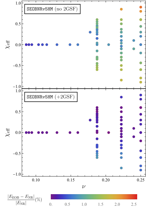
In Fig. 9 we compare the SEOBNRv5HM binding energy to the one extracted from NR simulations from Ref. 83. The SEOBNRv5HM with 2GSF corrections reproduces the NR binding energy much more faithfully, staying within the NR error estimates until roughly one GW cycle before merger. This improvement persists even when modeling aligned-spin binaries despite only adding 2GSF corrections to the nonspinning part of the waveform and RR force. In Fig. 10, we compare the SEOBNRv5HM binding energy for models with and without the 2GSF information to that of a set of spin-aligned NR waveforms 83 at a fixed value . Without the 2GSF calibration, the binding energy can be off by as much as 2.5% especially at high values of the effective spin . However, with the 2GSF calibration, we find deviations from the NR binding energy to be at the sub-percent level, with an average difference of just .
VI Discussion
In this paper, we have enhanced the accuracy of the (factorized) gravitational modes used in the SEORBNRv5 models of Refs. 65; 88; 94 by calibrating them to nonspinning, quasi-circular 2GSF multipolar data of Ref. 103. This calibration affects also the EOB radiation reaction (RR) force driving the dynamical evolution of the binary black holes in the SEORBNRv5 model.
By direct comparison of the energy flux in the SEORBNRv5HM model to that extracted from NR simulations, we have confirmed in Figs. 4 and 5 that the 2GSF calibration of the flux leads to a significant improvement in the faithfulness of the SEORBNRv5HM flux. In particular, the improvement seems to make the inclusion of NQC corrections in the RR force subdominant, and limited to the very late inspiral (plunge), where the effective test-body motion is almost unaffected by dissipative effects.
Furthermore, when looking at the mismatches between the SEORBNRv5HM and NR waveforms in Fig. 7, the inclusion of the 2GSF calibration seems to only have a marginal impact on the waveform mismatches after calibration to NR. If anything, this is a testament to the effectiveness of the SEORBNRv5 Hamiltonian’s calibration to NR, which is obtained by demanding that the mismatches of the SEORBNRv5 inspiral-merger-ringdown (2,2) modes are below . Since the waveforms are computed using the EOB equations of motion, which depend on the conservative and dissipative dynamics, the mismatches have significant degeneracy between the calibration terms in the EOB Hamiltonian and in the RR force (notably the 2GSF terms in the energy flux). This is one reason why the flux calibration terms that we have added to the EOB flux could not have been added through the NR calibration performed in Ref. 8866 6 One could explore in the future the possibility of calibrating directly the Hamiltonian from the binding energy extracted from NR simulations instead of doing it indirectly using the waveforms 83. However, this procedure would require the computation of the binding energy for the entire set of aligned-spin SXS NR waveforms used to calibrate the SEOBNRv5 model.. This degeneracy also means that calibrating SEOBNRv5HM to NR with and without the 2GSF calibration of the flux leads to a different EOB Hamiltonian. The Hamiltonian itself however is supposed to correspond to a gauge invariant observable of the binary, the binding energy. Comparing the EOB binding energy to results extracted from NR simulations in Fig. 9, we find that the Hamiltonian calibrated with the 2GSF information included reproduces the NR binding energy much more faithfully than the Hamiltonian calibrated without. This is a significant consistency test of the SEOBNRv5HM model, and one that extends to binary BHs with spins, as well (see Fig. 10). So, while adding the 2GSF information to the SEOBNRv5HM model does not necessarily improve the faithfulness of the corresponding waveforms in the regime where they are calibrated to NR, it does improve the overall consistency and naturalness of the model. This gives us greater confidence that the SEOBNRv5HM model will remain (somewhat) faithful to NR when extrapolated beyond the calibration region, in particular for higher mass ratios.
In this work we focused on adding 2GSF corrections to the nonspinning sector of the SEOBNRv5HM waveforms. However, numerical results are also available for corrections to the 2GSF flux linear in either the primary or secondary spin 103; 14; 71. In principle, the matching procedure employed here can also be used to calibrate the SEOBNRv5HM modes to these data. We will leave the implementation of this to future work.
A limiting factor in this work has been that the 2GSF multipolar flux data we used do not include corrections due to the transition from inspiral to plunge, causing it to diverge at the ISCO. This has limited our ability to calibrate the RR force and gravitational modes in the strong-field regime. Inclusion of these terms could lead to further improvements of our results, and will be addressed once new 2GSF data becomes available.
Acknowledgments
The authors thank Héctor Estellés, Mohammed Khalil, and Antoni Ramos-Buades for useful discussions. MvdM is supported by VILLUM FONDEN (grant no. 37766), and the Danish Research Foundation. NW acknowledges support from a Royal Society - Science Foundation Ireland University Research Fellowship. This publication has emanated from research conducted with the financial support of Science Foundation Ireland under Grant numbers 16/RS-URF/3428 and 17/RS-URF-RG/3490. AP acknowledges support from a Royal Society University Research Fellowship. For the purpose of Open Access, the authors have applied a CC BY public copyright licence to any Author Accepted Manuscript version arising from this submission. This work makes use of the Black Hole Perturbation Toolkit 34. Finally, the authors acknowledge the computational resources provided by the Max Planck Institute for Gravitational Physics (Albert Einstein Institute) in Potsdam, in particular, the Hypatia cluster. The SEOBNRv5 family of models is publicly available through the Python package pySEOBNR git.ligo.org/lscsoft/pyseobnr. Stable versions of pySEOBNR are published through the Python Package Index (PyPI), and can be installed via pip install pyseobnr.
Appendix A Independence of results on the specific EOB Hamiltonian
The accurate mismatches and small binding-energy disagreements with NR found in Sec. V have been obtained using the SEOBNRv5 nonspinning Hamiltonian of Ref. 65; 88. Here, we want to understand whether those results are somehow tied to the particular structure (or resummation) of the Hamiltonian and the PN content. Thus, we repeat some of the analyses using the non-spinning Hamiltonian from the previous SEOBNR family, SEOBNRv4 98; 38.
Figure 11 is similar to Fig. 7, but now we compute the mismatches between the SEOBNRv4.5HM and NR (2,2) waveforms, where the SEOBNRv4.5HM model is constructed calibrating the SEOBNRv4 Hamiltonian, and using the SEOBNRv5HM RR force and gravitational modes with and without the 2GSF information. We find that although the mismatches are a bit higher than for the SEOBNRv5 ones, there is actually a noticeable improvement when including the 2GSF information.
Appendix B Extended comparison between GSF and NR multipolar fluxes
In this appendix we show further comparisons between GSF and NR multipolar energy fluxes. The comparisons for the (3,2), (3,3), (4,3) and (4,4) modes are shown in Fig. 13. The residual after subtracting the GSF flux from the NR flux clearly shows the expected scaling. The comparisons for the (2,1) and (2,2) modes are presented in Fig. 14. The scaling of the residuals for these modes is less clear for the reasons given below and in the caption of the figure. The SXS datasets used to make Figs. 1, 13, and 14 are given in Table 1.
Figure 14 shows that for the (2,2) mode, the flux’s scaling with at is likely affected by the transition to plunge. Such a transition occurs over a frequency interval on a timescale , during which the small parameter enters into the SMR expansion 45. The behavior of the energy flux in this case can be obtained by combining Eq. (10) of Ref. 78 with Eqs. (22) and (23) of Ref. 21. In those equations, we define and , where is the orbital separation, such that and in the transition regime. The cited equations then give us
| (60) |
Here is the specific binding energy, meaning it is related to the flux by , which implies . (In all of these schematic equations, the reader should understand that powers of come with -dependent coefficients, which we omit to avoid introducing additional notation.) Figure 15 repeats the comparison in Fig. 14 at a frequency closer to the ISCO (), and there we see clear evidence of the term appearing in the flux.
Appendix C Numerical-relativity simulations
Throughout this paper we compare to NR simulations produced by the SXS collaboration.77 7 See the SXS Gravitational Waveform Database https://data.black-holes.org/waveforms/index.html. In Table 1, we provide some details of the NR simulations used in this paper. We selected all public SXS nonspinning quasicircular simulations with sufficiently different mass ratios, and initial eccentricity below . If more were available for the same parameters, we took the most recent one, or the second latest if that is at least 5 orbits longer.
| SXS ID | Used in Fig. | ||||
|---|---|---|---|---|---|
| SXS:BBH:2325 | 1.000 | 0.2500 | 5,6,7,11 | ||
| SXS:BBH:0198 | 1.202 | 0.2479 | 5,7,11 | ||
| SXS:BBH:0310 | 1.221 | 0.2475 | 5,7,11 | ||
| SXS:BBH:1143 | 1.250 | 0.2469 | 5,7,11 | ||
| SXS:BBH:2331 | 1.500 | 0.2400 | 5,7,11 | ||
| SXS:BBH:0194 | 1.518 | 0.2394 | 5,7,11 | ||
| SXS:BBH:1354 | 1.832 | 0.2284 | 5,7,11 | ||
| SXS:BBH:1165 | 2.000 | 0.2222 | 1,13,14,15 | ||
| SXS:BBH:2425 | 2.000 | 0.2222 | 5,7,11 | ||
| SXS:BBH:0201 | 2.316 | 0.2106 | 5,7,11 | ||
| SXS:BBH:0259 | 2.500 | 0.2041 | 1,5,7,11,13,14,15 | ||
| SXS:BBH:2265 | 3.000 | 0.1875 | 1,13,14,15 | ||
| SXS:BBH:2498 | 3.000 | 0.1875 | 5,7,11 | ||
| SXS:BBH:0200 | 3.272 | 0.1793 | 5,7,11 | ||
| SXS:BBH:2483 | 3.500 | 0.1728 | 1,5,7,11,13,14,15 | ||
| SXS:BBH:2485 | 3.999 | 0.1600 | 1,13,14,15 | ||
| SXS:BBH:1906 | 4.000 | 0.1600 | 1,13,14,15 | ||
| SXS:BBH:2499 | 4.000 | 0.1600 | 4,5,6,7,11 | ||
| SXS:BBH:1220 | 4.001 | 0.1600 | 1,13,14,15 | ||
| SXS:BBH:2484 | 4.500 | 0.1488 | 1,5,7,11,13,14,15 | ||
| SXS:BBH:2374 | 5.000 | 0.1389 | 5,7,11 | ||
| SXS:BBH:2487 | 5.000 | 0.1389 | 1,13,14,15 | ||
| SXS:BBH:0187 | 5.039 | 0.1381 | 5,7,11 | ||
| SXS:BBH:2486 | 5.500 | 0.1302 | 1,5,7,11,13,14,15 | ||
| SXS:BBH:0197 | 5.522 | 0.1298 | 5,7,11 | ||
| SXS:BBH:2489 | 5.999 | 0.1225 | 1,13,14,15 | ||
| SXS:BBH:2164 | 6.000 | 0.1225 | 5,7,11 | ||
| SXS:BBH:2488 | 6.500 | 0.1155 | 1,5,7,11,13,14,15 | ||
| SXS:BBH:0192 | 6.580 | 0.1145 | 5,7,11 | ||
| SXS:BBH:2491 | 7.000 | 0.1094 | 1,5,7,11,13,14,15 | ||
| SXS:BBH:0188 | 7.187 | 0.1072 | 5,7,11 | ||
| SXS:BBH:2490 | 7.500 | 0.1038 | 1,7,11,13,14,15 | ||
| SXS:BBH:0195 | 7.761 | 0.1011 | 5,7,11 | ||
| SXS:BBH:2493 | 8.000 | 0.09876 | 1,5,7,11,13,14,15 | ||
| SXS:BBH:0186 | 8.267 | 0.09626 | 5,7,11 | ||
| SXS:BBH:2492 | 8.501 | 0.09417 | 1,5,7,11,13,14,15 | ||
| SXS:BBH:0199 | 8.729 | 0.09222 | 5,7,11 | ||
| SXS:BBH:2495 | 9.001 | 0.08999 | 1,5,7,11,13,14,15 | ||
| SXS:BBH:0189 | 9.167 | 0.08868 | 5,7,11 | ||
| SXS:BBH:1108 | 9.200 | 0.08843 | 5,7,11 | ||
| SXS:BBH:2494 | 9.497 | 0.08619 | 1,5,7,11,13,14,15 | ||
| SXS:BBH:0196 | 9.663 | 0.08499 | 5,7,11 | ||
| SXS:BBH:0185 | 9.990 | 0.08271 | 5,6,7,11 | ||
| SXS:BBH:1107 | 10.00 | 0.08264 | 1,13,14,15 | ||
| SXS:BBH:2480 | 14.00 | 0.06222 | 1,5,7,11,13,14,15 | ||
| SXS:BBH:2477 | 15.00 | 0.05859 | 1,5,7,11,13,14,15 | ||
| SXS:BBH:2516 | 20.00 | 0.04536 | 1,5,7,11,13,14,15 |
References
- Advanced LIGO. Class. Quant. Grav. 32, pp. 074001. External Links: Document, 1411.4547 Cited by: §I.
- Binary Black Hole Mergers in the first Advanced LIGO Observing Run. Phys. Rev. X6 (4), pp. 041015. Note: [erratum: Phys. Rev.X8,no.3,039903(2018)] External Links: Document, 1606.04856 Cited by: §I.
- Prospects for observing and localizing gravitational-wave transients with Advanced LIGO, Advanced Virgo and KAGRA. Living Rev. Rel. 21 (1), pp. 3. External Links: 1304.0670, Document Cited by: §I.
- Binary Black Hole Population Properties Inferred from the First and Second Observing Runs of Advanced LIGO and Advanced Virgo. Astrophys. J. Lett. 882 (2), pp. L24. External Links: 1811.12940, Document Cited by: §I, §I.
- GWTC-1: A Gravitational-Wave Transient Catalog of Compact Binary Mergers Observed by LIGO and Virgo during the First and Second Observing Runs. Phys. Rev. X9 (3), pp. 031040. External Links: Document, 1811.12907 Cited by: §I.
- GW190412: Observation of a Binary-Black-Hole Coalescence with Asymmetric Masses. Phys. Rev. D 102 (4), pp. 043015. External Links: 2004.08342, Document Cited by: §I.
- GW190814: Gravitational Waves from the Coalescence of a 23 Solar Mass Black Hole with a 2.6 Solar Mass Compact Object. Astrophys. J. Lett. 896 (2), pp. L44. External Links: 2006.12611, Document Cited by: §I.
- GWTC-2: Compact Binary Coalescences Observed by LIGO and Virgo During the First Half of the Third Observing Run. Phys. Rev. X 11, pp. 021053. External Links: 2010.14527, Document Cited by: §I.
- Population Properties of Compact Objects from the Second LIGO-Virgo Gravitational-Wave Transient Catalog. Astrophys. J. Lett. 913 (1), pp. L7. External Links: 2010.14533, Document Cited by: §I.
- GWTC-3: Compact Binary Coalescences Observed by LIGO and Virgo during the Second Part of the Third Observing Run. Phys. Rev. X 13 (4), pp. 041039. External Links: 2111.03606, Document Cited by: §I.
- GWTC-2.1: Deep extended catalog of compact binary coalescences observed by LIGO and Virgo during the first half of the third observing run. Phys. Rev. D 109 (2), pp. 022001. External Links: 2108.01045, Document Cited by: §I.
- Advanced Virgo: a second-generation interferometric gravitational wave detector. Class. Quant. Grav. 32 (2), pp. 024001. External Links: Document, 1408.3978 Cited by: §I.
- Gravitational self-force and the effective-one-body formalism between the innermost stable circular orbit and the light ring. Phys. Rev. D 86, pp. 104041. External Links: 1209.0964, Document Cited by: §I, §IV.
- Dissipation in extreme-mass ratio binaries with a spinning secondary. Phys. Rev. D 102 (6), pp. 064013. External Links: 1912.09461, Document Cited by: §VI.
- Numerical computation of the EOB potential q using self-force results. Phys. Rev. D93 (6), pp. 064063. External Links: Document, 1512.03392 Cited by: §I.
- Frequency-domain algorithm for the Lorenz-gauge gravitational self-force. Phys. Rev. D 88 (10), pp. 104009. External Links: 1308.5223, Document Cited by: §III.
- A Fast Frequency-Domain Algorithm for Gravitational Self-Force: I. Circular Orbits in Schwarzschild Spacetime. Phys. Rev. D 83, pp. 124026. External Links: 1012.5860, Document Cited by: §III.
- KAGRA: 2.5 Generation Interferometric Gravitational Wave Detector. Nature Astron. 3 (1), pp. 35–40. External Links: 1811.08079, Document Cited by: §I.
- Overview of KAGRA: Detector design and construction history. PTEP 2021 (5), pp. 05A101. External Links: 2005.05574, Document Cited by: §I.
- Comparing second-order gravitational self-force and effective one body waveforms from inspiralling, quasicircular and nonspinning black hole binaries. II. The large-mass-ratio case. Phys. Rev. D 106 (8), pp. 084062. External Links: 2208.02055, Document Cited by: §I, §V.
- Comparing second-order gravitational self-force, numerical relativity, and effective one body waveforms from inspiralling, quasicircular, and nonspinning black hole binaries. Phys. Rev. D 106 (8), pp. 084061. External Links: 2208.01049, Document Cited by: Appendix B, §I, §III, §III, §V, footnote 2, footnote 4.
- Quasicircular inspirals and plunges from nonspinning effective-one-body Hamiltonians with gravitational self-force information. Phys. Rev. D 101 (2), pp. 024024. External Links: 1907.11597, Document Cited by: §I, §IV.
- Gravitational wave extraction from an inspiraling configuration of merging black holes. Phys. Rev. Lett. 96, pp. 111102. External Links: gr-qc/0511103, Document Cited by: §I.
- Perturbations of Schwarzschild black holes in the Lorenz gauge: Formulation and numerical implementation. Phys. Rev. D 72, pp. 104026. External Links: gr-qc/0510019, Document Cited by: §III.
- Gravitational self force on a particle in circular orbit around a Schwarzschild black hole. Phys. Rev. D 75, pp. 064021. External Links: gr-qc/0701069, Document Cited by: §III.
- Gravitational self-force correction to the innermost stable circular orbit of a Schwarzschild black hole. prl 102, pp. 191101. External Links: Document, 0902.0573 Cited by: §I.
- The complete non-spinning effective-one-body metric at linear order in the mass ratio. Phys. Rev. D 85, pp. 064010. External Links: 1111.5610, Document Cited by: §I, §IV.
- Rotating black holes: Locally nonrotating frames, energy extraction, and scalar synchrotron radiation. Astrophys. J. 178, pp. 347. External Links: Document Cited by: §II.2.
- Updated advanced ligo sensitivity design curve. Note: LIGO Document T1800044-v5 External Links: Link Cited by: §V.
- Novel approach to binary dynamics: application to the fifth post-Newtonian level. Phys. Rev. Lett. 123 (23), pp. 231104. External Links: 1909.02375, Document Cited by: §II.1.
- Binary dynamics at the fifth and fifth-and-a-half post-Newtonian orders. Phys. Rev. D 102 (2), pp. 024062. External Links: 2003.11891, Document Cited by: §II.1.
- Sixth post-Newtonian local-in-time dynamics of binary systems. Phys. Rev. D 102 (2), pp. 024061. External Links: 2004.05407, Document Cited by: §II.1.
- Sixth post-Newtonian nonlocal-in-time dynamics of binary systems. Phys. Rev. D 102 (8), pp. 084047. External Links: 2007.11239, Document Cited by: §II.1.
- [34] Black Hole Perturbation Toolkit. Note: (bhptoolkit.org) Cited by: Acknowledgments.
- Gravitational wave tails of tails. Class. Quant. Grav. 15, pp. 113–141. Note: [Erratum: Class.Quant.Grav. 22, 3381 (2005)] External Links: gr-qc/9710038, Document Cited by: §II.2.
- Gravitational Radiation from Post-Newtonian Sources and Inspiralling Compact Binaries. Living Rev. Rel. 17, pp. 2. External Links: 1310.1528, Document Cited by: §I.
- The fifth-order post-Newtonian Hamiltonian dynamics of two-body systems from an effective field theory approach. Nucl. Phys. B 983, pp. 115900. Note: [Erratum: Nucl.Phys.B 985, 115991 (2022)] External Links: 2110.13822, Document Cited by: §II.1.
- Improved effective-one-body model of spinning, nonprecessing binary black holes for the era of gravitational-wave astrophysics with advanced detectors. Phys. Rev. D 95 (4), pp. 044028. External Links: 1611.03703, Document Cited by: Appendix A, §I, §I.
- The SXS Collaboration catalog of binary black hole simulations. Class. Quant. Grav. 36 (19), pp. 195006. External Links: 1904.04831, Document Cited by: §V, §V.
- Effective one-body approach to general relativistic two-body dynamics. Phys. Rev. D 59, pp. 084006. External Links: gr-qc/9811091, Document Cited by: §I, §I, §II.1, §II.1.
- Transition from inspiral to plunge in precessing binaries of spinning black holes. Phys. Rev. D 74, pp. 104005. External Links: gr-qc/0508067, Document Cited by: §I, §II.3.
- Transition from inspiral to plunge in binary black hole coalescences. Phys. Rev. D 62, pp. 064015. External Links: gr-qc/0001013, Document Cited by: §I, §II.1.
- Effective-one-body waveforms calibrated to numerical relativity simulations: Coalescence of non-spinning, equal-mass black holes. Phys. Rev. D 79, pp. 124028. External Links: 0902.0790, Document Cited by: §II.2.
- Accurate evolutions of orbiting black-hole binaries without excision. Phys. Rev. Lett. 96, pp. 111101. External Links: gr-qc/0511048, Document Cited by: §I.
- Asymptotically matched quasi-circular inspiral and transition-to-plunge in the small mass ratio expansion. SciPost Phys. 13 (2), pp. 043. External Links: 2112.02114, Document Cited by: Appendix B, §III.
- Enriching the Symphony of Gravitational Waves from Binary Black Holes by Tuning Higher Harmonics. Phys. Rev. D 98 (8), pp. 084028. External Links: 1803.10701, Document Cited by: §I, §I, §II.2.
- Gravitational waves from black hole binary inspiral and merger: The Span of third postNewtonian effective one-body templates. Phys. Rev. D 67, pp. 064028. External Links: gr-qc/0211041, Document Cited by: §II.2.
- Improved resummation of post-Newtonian multipolar waveforms from circularized compact binaries. Phys. Rev. D 79, pp. 064004. External Links: 0811.2069, Document Cited by: §II.2, §II.3, §IV, §IV.
- On the determination of the last stable orbit for circular general relativistic binaries at the third postNewtonian approximation. Phys. Rev. D 62, pp. 084011. External Links: gr-qc/0005034, Document Cited by: §I, §I, §II.1.
- Fourth post-Newtonian effective one-body dynamics. Phys. Rev. D 91 (8), pp. 084024. External Links: 1502.07245, Document Cited by: §II.1.
- Accurate Effective-One-Body waveforms of inspiralling and coalescing black-hole binaries. Phys. Rev. D 78, pp. 044039. External Links: 0803.3162, Document Cited by: §II.2.
- Faithful effective-one-body waveforms of small-mass-ratio coalescing black-hole binaries. Phys. Rev. D 76, pp. 064028. External Links: 0705.2519, Document Cited by: §II.2.
- Comparing Effective-One-Body gravitational waveforms to accurate numerical data. Phys. Rev. D 77, pp. 024043. External Links: 0711.2628, Document Cited by: §II.2.
- Coalescence of two spinning black holes: an effective one-body approach. Phys. Rev. D 64, pp. 124013. External Links: gr-qc/0103018, Document Cited by: §I.
- Gravitational Self Force in a Schwarzschild Background and the Effective One Body Formalism. Phys. Rev. D 81, pp. 024017. External Links: 0910.5533, Document Cited by: §I.
- High-energy gravitational scattering and the general relativistic two-body problem. Phys. Rev. D97 (4), pp. 044038. External Links: Document, 1710.10599 Cited by: §I.
- A Consequence of the gravitational self-force for circular orbits of the Schwarzschild geometry. Phys. Rev. D 77, pp. 124026. External Links: 0804.3529, Document Cited by: §IV.
- Slow evolution of the metric perturbation due to a quasicircular inspiral into a Schwarzschild black hole. Phys. Rev. D 106 (8), pp. 084023. External Links: 2206.08179, Document Cited by: §III.
- Observing binary inspiral in gravitational radiation: One interferometer. Phys. Rev. D 47, pp. 2198–2219. External Links: gr-qc/9301003, Document Cited by: §V.
- Gravitational Waves from a Particle in Circular Orbits around a Schwarzschild Black Hole to the 22nd Post-Newtonian Order. Prog. Theor. Phys. 128, pp. 971–992. External Links: 1211.5535, Document Cited by: §IV.
- Effective-one-body waveforms for precessing coalescing compact binaries with post-Newtonian twist. Phys. Rev. D 106 (2), pp. 024020. External Links: 2111.03675, Document Cited by: §I.
- Two timescale analysis of extreme mass ratio inspirals in Kerr. I. Orbital Motion. Phys. Rev. D 78, pp. 064028. External Links: 0805.3337, Document Cited by: §III.
- The final spin from binary black holes in quasi-circular orbits. Astrophys. J. Lett. 825 (2), pp. L19. External Links: 1605.01938, Document Cited by: §II.2.
- Hierarchical data-driven approach to fitting numerical relativity data for nonprecessing binary black holes with an application to final spin and radiated energy. Phys. Rev. D 95 (6), pp. 064024. External Links: 1611.00332, Document Cited by: §II.2.
- Theoretical groundwork supporting the precessing-spin two-body dynamics of the effective-one-body waveform models SEOBNRv5. Phys. Rev. D 108 (12), pp. 124036. External Links: 2303.18143, Document Cited by: Appendix A, §I, §II.1, §VI.
- Gravitational Self-Force Correction to the Binding Energy of Compact Binary Systems. Phys. Rev. Lett. 108, pp. 131103. External Links: 1111.5609, Document Cited by: §I, §IV.
- The First Law of Binary Black Hole Mechanics in General Relativity and Post-Newtonian Theory. Phys. Rev. D 85, pp. 064039. External Links: 1111.5378, Document Cited by: §I, §IV.
- Periastron Advance in Black Hole Binaries. Phys. Rev. Lett. 107, pp. 141101. External Links: 1106.3278, Document Cited by: §III.
- First Law of Mechanics for Compact Binaries on Eccentric Orbits. Phys. Rev. D 92 (8), pp. 084021. External Links: 1506.05648, Document Cited by: §I.
- Effective Field Theories of Post-Newtonian Gravity: A comprehensive review. Rept. Prog. Phys. 83 (7), pp. 075901. External Links: 1807.01699, Document Cited by: §I.
- Self-force calculations with a spinning secondary. Phys. Rev. D 105 (8), pp. 084031. External Links: 2112.13069, Document Cited by: §VI.
- pySEOBNR: a software package for the next generation of effective-one-body multipolar waveform models. . External Links: 2303.18203 Cited by: §I.
- Two-timescale evolution of extreme-mass-ratio inspirals: waveform generation scheme for quasicircular orbits in Schwarzschild spacetime. Phys. Rev. D 103 (6), pp. 064048. External Links: 2006.11263, Document Cited by: §III, §III.
- Second-order perturbation theory: the problem of infinite mode coupling. Phys. Rev. D 94 (10), pp. 104018. External Links: 1608.06783, Document Cited by: §III.
- Toward a gravitational self-force-informed effective-one-body waveform model for nonprecessing, eccentric, large-mass-ratio inspirals. Phys. Rev. D 106 (6), pp. 064049. External Links: 2207.14002, Document Cited by: §I.
- Time-domain effective-one-body gravitational waveforms for coalescing compact binaries with nonprecessing spins, tides and self-spin effects. Phys. Rev. D 98 (10), pp. 104052. External Links: 1806.01772, Document Cited by: §I, §I.
- Multipolar effective one body waveform model for spin-aligned black hole binaries. Phys. Rev. D 102 (2), pp. 024077. External Links: 2001.09082, Document Cited by: §I, §I.
- Success of the small mass-ratio approximation during the final orbits of binary black hole simulations. Phys. Rev. D 107 (8), pp. 084021. External Links: 2207.04066, Document Cited by: Appendix B.
- 1-OGC: The first open gravitational-wave catalog of binary mergers from analysis of public Advanced LIGO data. Astrophys. J. 872 (2), pp. 195. External Links: 1811.01921, Document Cited by: §I.
- 2-OGC: Open Gravitational-wave Catalog of binary mergers from analysis of public Advanced LIGO and Virgo data. Astrophys. J. 891, pp. 123. External Links: 1910.05331, Document Cited by: §I.
- 4-OGC: Catalog of Gravitational Waves from Compact Binary Mergers. Astrophys. J. 946 (2), pp. 59. External Links: 2112.06878, Document Cited by: §I.
- New binary black hole mergers in the LIGO-Virgo O3a data. Phys. Rev. D 106 (4), pp. 043009. External Links: 2201.02252, Document Cited by: §I.
- Assessing the Energetics of Spinning Binary Black Hole Systems. Phys. Rev. D 98 (10), pp. 104057. External Links: 1712.06533, Document Cited by: §V, footnote 6.
- Multipolar Effective-One-Body Waveforms for Precessing Binary Black Holes: Construction and Validation. Phys. Rev. D 102 (4), pp. 044055. External Links: 2004.09442, Document Cited by: §I, §II.3.
- Inspiral-merger-ringdown multipolar waveforms of nonspinning black-hole binaries using the effective-one-body formalism. Phys. Rev. D 84, pp. 124052. External Links: 1106.1021, Document Cited by: §II.3.
- Post-Newtonian factorized multipolar waveforms for spinning, non-precessing black-hole binaries. Phys. Rev. D 83, pp. 064003. Note: [Erratum: Phys.Rev.D 87, 109901 (2013)] External Links: 1006.0431, Document Cited by: §II.2.
- The Motion of point particles in curved spacetime. Living Rev. Rel. 14, pp. 7. External Links: 1102.0529, Document Cited by: §I.
- Laying the foundation of the effective-one-body waveform models SEOBNRv5: Improved accuracy and efficiency for spinning nonprecessing binary black holes. Phys. Rev. D 108 (12), pp. 124035. External Links: 2303.18039, Document Cited by: Appendix A, §I, §II.1, §II.2, §II.2, §II.3, §II.3, §II, §IV, Figure 6, §V, §V, §V, §V, §V, §VI, §VI, footnote 3.
- The effective field theorist’s approach to gravitational dynamics. Phys. Rept. 633, pp. 1–104. External Links: 1601.04914, Document Cited by: §I.
- Practical, covariant puncture for second-order self-force calculations. Phys. Rev. D 89 (10), pp. 104020. External Links: 1403.1843, Document Cited by: §III.
- Second-Order Self-Force Calculation of Gravitational Binding Energy in Compact Binaries. Phys. Rev. Lett. 124 (2), pp. 021101. External Links: 1908.07419, Document Cited by: §III.
- Second-order perturbation theory: problems on large scales. Phys. Rev. D 92 (10), pp. 104047. External Links: 1510.05172, Document Cited by: §III.
- Evolution of binary black hole spacetimes. Phys. Rev. Lett. 95, pp. 121101. External Links: gr-qc/0507014, Document Cited by: §I.
- Next generation of accurate and efficient multipolar precessing-spin effective-one-body waveforms for binary black holes. Phys. Rev. D 108 (12), pp. 124037. External Links: 2303.18046, Document Cited by: §I, §VI.
- Assessment of consistent next-to-quasicircular corrections and postadiabatic approximation in effective-one-body multipolar waveforms for binary black hole coalescences. Phys. Rev. D 104 (10), pp. 104045. External Links: 2104.07533, Document Cited by: §II.3.
- Choice of filters for the detection of gravitational waves from coalescing binaries. Phys. Rev. D 44, pp. 3819–3834. External Links: Document Cited by: §V.
- Hamiltonian formulation of general relativity and post-Newtonian dynamics of compact binaries. Living Rev. Rel. 21 (1), pp. 7. External Links: 1805.07240, Document Cited by: §I.
- Effective-one-body model for black-hole binaries with generic mass ratios and spins. Phys. Rev. D 89 (6), pp. 061502. External Links: 1311.2544, Document Cited by: Appendix A, §I, §II.3.
- Intermediate mass-ratio black hole binaries: Applicability of small mass-ratio perturbation theory. Phys. Rev. Lett. 125 (18), pp. 181101. External Links: 2006.12036, Document Cited by: §III.
- Metric perturbations produced by eccentric equatorial orbits around a Kerr black hole. Phys. Rev. D 92 (6), pp. 064025. External Links: 1506.04755, Document Cited by: §IV, §IV.
- Comparison of binary black hole initial data sets. Phys. Rev. D 98 (10), pp. 104011. External Links: 1808.08228, Document Cited by: §V.
- New binary black hole mergers in the second observing run of Advanced LIGO and Advanced Virgo. Phys. Rev. D 101 (8), pp. 083030. External Links: 1904.07214, Document Cited by: §I.
- Gravitational-Wave Energy Flux for Compact Binaries through Second Order in the Mass Ratio. Phys. Rev. Lett. 127 (15), pp. 151102. External Links: 2107.01298, Document Cited by: §I, §III, §III, §VI, §VI.
- Gravitational Waveforms for Compact Binaries from Second-Order Self-Force Theory. Phys. Rev. Lett. 130 (24), pp. 241402. External Links: 2112.12265, Document Cited by: §I, §III, §V.
- Applying the effective-source approach to frequency-domain self-force calculations: Lorenz-gauge gravitational perturbations. Phys. Rev. D 92 (8), pp. 084019. External Links: 1505.07841, Document Cited by: §III.
- Modeling Extreme Mass Ratio Inspirals within the Effective-One-Body Approach. Phys. Rev. Lett. 104, pp. 091102. External Links: 0909.4263, Document Cited by: §I.
- Extreme Mass-Ratio Inspirals in the Effective-One-Body Approach: Quasi-Circular, Equatorial Orbits around a Spinning Black Hole. Phys. Rev. D 83, pp. 044044. Note: [Erratum: Phys.Rev.D 88, 109904 (2013)] External Links: 1009.6013, Document Cited by: §I.
- Detecting gravitational waves with disparate detector responses: Two new binary black hole mergers. Phys. Rev. D 104 (6), pp. 063030. External Links: 1910.09528, Document Cited by: §I.