Hydrodynamics of a relativistic charged fluid in the presence of a periodically modulated chemical potential
N. Chagnet1, K. Schalm1
1 Instituut-Lorentz for Theoretical Physics, -ITP, Leiden University, The Netherlands.
⋆ chagnet@lorentz.leidenuniv.nl
March 30, 2023
Abstract
We study charged hydrodynamics in a periodic lattice background. Fluctuations are Bloch waves rather than single momentum Fourier modes. At boundaries of the unit cell where hydrodynamic fluctuations are formally degenerate with their Umklapped copy, level repulsion occurs. Novel mode mixings between charge, sound, and their Umklapped copies appear at finite chemical potential — both at zero and finite momentum. We provide explicit examples for an ionic lattice, i.e. a periodic external chemical potential, and verify our results with numerical computations in fluid-gravity duality.
1 Introduction
In considering the quantum mechanical wave function of a single electron in a lattice of atoms Bloch had the insight that one should expand the wavefunction in a manner consistent with the discrete periodicity11 1 The Fourier transform here is chosen with a different convention than the traditional physics convention . This prevents a proliferation of -factors in non-linear terms in dynamical fluctuation equations.
| (1) |
The novel part of Bloch was its application to quantum wavefunctions rather than waves in general. How waves propagate in periodic structures was already considered by Newton, and that waves in periodic structures exhibit peculiar interference phenomena that we now know as level repulsion/Umklapp/gap opening at Brillouin zone boundaries or Bragg reflection from point-like lattices was already recognized by Kelvin in the 1880s [1]. In electrical engineering the propagation of electromagnetic waves in periodic structures was [2], and is an important topic, see e.g. [3].22 2 In the latter context Bloch’s theorem is known as Floquet’s theorem. This is not to be confused with periodically driven Floquet systems, though the underlying mathematics of periodic structures is the same after switching “space” and “time”. Also sound waves in lattices were considered from the earliest days up to today, see e.g. [4].
Sound waves, however, are hydrodynamic fluctuations – a long-time long-wavelength perturbation around thermodynamic equilibrium of a conserved charge associated to a global symmetry – and in that sense differ from electromagnetic waves or single particle wavefunctions in that the fundamental equations of motion, i.e. the hydrodynamic conservation laws, are non-linear. The wave-like fluctuations propagate on a background that is itself a full (equilibrium) solution to the non-linear set of equations, and through the non-linearity the properties of the fluctuating waves depend on this background solution. Though gradients are energetically disfavored, through external forcing the equilibrium background can be imprinted with a spatially varying temperature , pressure , or chemical potential . Due to the non-linear coupling between fluctuations and the background in hydrodynamics, the wave propagation properties can be self-consistently determined from the (spatially varying) background. This was elucidated particularly clearly in recent years in the context of electron hydrodynamics in systems with random charge impurities [5, 6]. Such charge disorder is encoded in a spatially varying chemical potential with average and variance . Quantum mechanical single particle electron motion in the presence of random impurities is a classic condensed matter problem. As Anderson showed, the random wavefunction interference is essentially uniformly destructive; at low temperatures all motion is inhibited and the system becomes an insulator. In the hydrodynamic regime, however, i.e., in a situation where many electrons collectivize to a classical fluid rather than a quantum mechanical wave, the conductivity rather strikingly remains finite indicating the existence of an “incoherent metal” state [6]. Observing this electron hydrodynamics in sufficiently pure 2D systems is currently actively pursued, see e.g. [7] or [8], references therein and the recent review [9].
Here we study not hydrodynamics with random spatial disorder but with strictly periodic modulations of the background, i.e. a lattice. Moreover, we also consider hydrodynamics of a charged rather than a neutral fluid with an eye towards condensed matter systems. Compared to the many existing studies on sound waves in periodic structures, the presence of electromagnetic charge as an additional conserved quantum number changes the fluctuating wave response fundamentally. This is again due to the non-linear nature of the hydrodynamic equations. At finite chemical potential sound mixes with charge diffusion. In a companion article we focus on the significant consequences of this cross-coupling of Bloch modes in a lattice for the measurable DC and AC conductivities in condensed matter systems where this hydrodynamics approach may apply [10]. In this article we provide the deeper hydrodynamic analysis of the full fluctuation spectrum of charged hydrodynamics in a periodic background.
2 Hydrodynamics: Set-up and brief review of homogeneous fluctuations
The principal reason that linearized hydrodynamic fluctuations in a lattice background should also be expanded in Bloch modes has already been emphasized: the essence is wave propagation in a periodic structure. Waves are described by coupled first order differential equations of the form 33 3 The standard wave equation follows from (2)
| (3) |
If is periodic , then can be decomposed in Bloch waves44 4 The Bloch theorem essentially states that the plane wave decomposition can be segmented into unit cells where labels each cell – or Brillouin zone – as . The wavevector in each Brillouin zone can be shifted with such that (4) The advantage of this decomposition is that discrete periodic shifts relate modes in different Brillouin zones at the same Bloch momentum . . Taking as canonical example, one can solve Eq. (3) perturbatively in . Diagonalizing in terms of , the lowest eigenvector to first order in is
| (5) |
in terms of the unperturbed eigenmodes. This mixing between the different Bloch waves is Umklapp. In this article we shall only focus on these perturbative solutions for small lattice amplitudes.
We also already noted that what is special about hydrodynamics is that the fluctuation equations are themselves a linearization expansion of the fundamental non-linear equations. The principle behind the theory of hydrodynamics is local equilibrium and encoded in the local conservation laws of macroscopic charges, i.e., of a slowly spatially varying energy-momentum tensor and in the presence of a charge, a current . In turn this implies that one can also describe fluid behavior in the presence of a slowly spatially varying external potential whether temperature , pressure , or chemical potential .
For simplicity — as well as for the experimental supposition that strongly correlated condensed matter systems can have an emergent Lorentz symmetry at low energies — we shall use relativistic charged hydrodynamics in this article. In principle all we state also applies to arbitrary non-relativistic charged hydrodynamics, even if the precise expressions may be subtly different. In relativistic charged hydrodynamics the dynamical equations are simply the conservation equation of the energy-momentum tensor and the charge-current
| (6) |
Here we have allowed for an external electromagnetic field strength in terms of a local external vector potential. In this paper, we will be interested in taking with a periodic function. Though again, in principle our results also hold for a spatially varying (external) pressure (see e.g. [11]), or a spatially varying (external) temperature.55 5 A spatially varying temperature without forcing by contact with a spatially varying heatbath is difficult to have in a static equilibrium configuration, however.
The dynamical variables of the fluid are the temperature , the unit timelike velocity vector , and the chemical potential . Away from equilibrium, the conserved currents in our theory – which we assumed to be parity-invariant, see [12] for more general cases – are given by the constitutive relations at first order in gradients in Landau frame
| (7a) | ||||
| (7b) | ||||
Here is the number of spatial dimensions and the shear viscosity , the bulk viscosity , and the microscopic conductivity are hydrodynamic transport coefficients — in principle set by the microscopic details of a given theory, see e.g. [13, 14], in practice phenomenologically determined. is a projector orthogonal to the fluid velocity. The Landau frame choice is such that at any order in gradients, we have and .
The above constitutive relations also hold in a static equilibrium background. In a system with Galilean or relativistic Lorentz boost invariance — which we use in this paper — it is convenient to choose the reference frame for which the equilibrium fluid is at rest. In absence of contact to a spatially varying heat bath, the temperature must then also be constant and independent of position. In the presence of a spatially varying external chemical potential , the equilibrium solution to the hydrodynamic equations Eqs. (6) is then parametrized as
| (8) |
In the grand canonical ensemble, the hydrostatic equilibrium yields moreover
| (9) |
Throughout this paper we will use the bar notation to denote such static background quantities. For a homogeneous background, they will be spatially constant and we will use a subscript as to denote them. For spatially varying quantities, we will use superscripts to describe higher order (Bloch wave) moments
| (10) |
The hydrodynamic equations need to be supplemented by an equilibrium equation of state relating the energy density , the pressure and the charge density to solve in terms of the equilibrium values of and . In this paper, we will be considering a general fluid whose equation of state determines the thermodynamic equilibrium of the theory. In Sec. 4, we will specialize to conformal systems.
On top of this background, we now consider perturbations . The conservation equations (6) then take the form
| (11a) | ||||
| (11b) | ||||
| (11c) | ||||
| (11d) | ||||
which can further be simplified into
| (12a) | ||||
| (12b) | ||||
| (12c) | ||||
| (12d) | ||||
In the previous expression, we have defined a renormalized viscosity . We also introduced the “potential”-variations and conjugate to the energy and charge densities. The velocity perturbations are conjugate to the momenta . These are not independent due to the hydrodynamic local equilibrium condition. The momenta are related to the velocity perturbations through the constitutive relations at this order.66 6 Formally the susceptibility denotes how a local charge density is influenced by a (chemical) potential at a different space-time point. Here is the partition function in the presence of a chemical potential (velocity) for the charge density (momentum) . In the hydrodynamic limit, however, one assumes that all equilibrium () static () charges depend only locally on the potentials . In a homogeneous equilibrium background where this is equivalent to approximating the static susceptibility with its constant part . We discuss this in more detail below and in Appendix A. Similarly, the charge and energy densities are related to the sources through the thermodynamic susceptibilities derived in Appendix A. Using that , we can use the fundamental thermodynamic relation and the first law of thermodynamics to relate
| (13) |
Finally, we introduced an external electric field and in (12) we introduced the total electric field . In what follows, we will be interested in the hydrodynamics response of the modes obeying the equations (12). In the following sections, we will use the static susceptibilities relating the potentials to the densities to express the equations in terms of the latter only, i.e., we work in the microcanonical ensemble.
2.1 Hydrodynamic fluctuations in a homogeneous background
In this section, we first review the hydrodynamics of a long wavelength perturbation above a homogeneous conformal charged fluid. Further details can be found in [15, 16]. Since the background is homogeneous, this means every barred quantity will be a constant . The equations (12) decouple into the longitudinal and transverse sectors. We will start by looking at the latter whose equation of motion is simpler. Choosing the wavenumber along the direction without loss of generality, the transverse fluctuations obey
| (14) |
This is a simple diffusion equation with the shear diffusion constant . We can now use the (Fourier-)Laplace transform77 7 The Laplace transform is required to have a well-defined right-hand side to our linearized equations. One could also just use a Fourier transform while setting external sources. More details can be found in [15, 16]. such that the transverse equation of motion becomes
| (15) |
The solution is formally given in terms of the retarded correlator for the transverse momentum which is defined as
| (16) |
Using that in the hydrodynamic long wavelength limit (i.e., we only keep the leading term in an expansion in ; see footnote 6.), we have
| (17) |
The correlator exhibits a pole on the imaginary axis at indicative of a purely diffusive mode.
We can now carry the same analysis in the longitudinal sector where the dynamical equations are coupled. Denoting , the dynamical equations can be written succinctly as
| (18) |
We can once again use a (Fourier)-Laplace transform to rewrite this system of equations as
| (19) |
with the dynamical matrix
| (20) |
where we defined the determinant of the susceptibility matrix in the sector. The poles of the Green’s functions associated to this system are the frequencies for which . The roots of this polynomial in the long wavelength limit are a diffusion mode (originating in charge diffusion) and two propagating sound modes
| (21) |
where the speed of sound and the two diffusion constants are defined as
| (22a) | ||||
| (22b) | ||||
Note that for the speed of sound reduces to the familiar expression (using Eq. (13) and the inverse susceptibility matrix). Similarly to what we did in the transverse sector, we can compute the retarded Green’s functions by inverting the dynamical system [16]
| (23) |
where the middle equation enforces the condition that the static part reduces to the longitudinal part of the thermodynamic susceptibility matrix . The various correlators can then be obtained
| (24a) | ||||
| (24b) | ||||
| (24c) | ||||
| (24d) | ||||
with the normalized determinant of the dynamical matrix . The other correlators can be obtained via the Ward identities
| (25) |
as well as the Onsager reciprocal relations
| (26) |
3 Hydrodynamic fluctuations in a lattice background
We shall now redo the fluctuation analysis in a lattice background. This lattice will be sourced by a periodically modulated external chemical potential
| (27) |
such that the fluid is still at rest and in local equilibrium, but all its constituents will now slowly vary in space. In particular, this last assumption of local equilibrium means that the scale of spatial fluctuations of and other local quantities must be larger than the local equilibration scale. Therefore, we must have .88 8 For this reason our analysis does not immediately apply to graphene or other sufficiently pure semi-metals as there the scale where hydrodynamics applies is much larger than the atomic lattice scale. One would need to have a periodically undulating graphene sheet or otherwise externally imposed periodicity for this analysis to apply.
This lattice background manifestly breaks translation invariance. Momentum is therefore no longer a strictly conserved quantity. However, as the breaking is sourced through a hydrodynamic variable and as we assume it is weakly broken, we can still use hydrodynamic analysis [6, 5, 17, 18]. The spectral function of the associated operator to this deformation — the charge density —, evaluated in the homogeneous background, can be used to compute the momentum relaxation rate. This is known as the memory matrix formalism and was thoroughly detailed in e.g. [19, 5]. The momentum relaxation rate induced by an operator sourced at wavenumber with strength takes the form [20]
| (28) |
For a cosine ionic lattice Eq. (27), , and we have two deformation sources, one copy each at — noting that the expression (28) is parity invariant in . Therefore, the memory matrix relaxation rate for an ionic lattice is
| (29) |
It will prove useful to separate the terms according to their scaling with in this expression as with
| (30) |
Using the Einstein relations Eq. (22a), together with these are a convective shear drag term and an intrinsic diffusive term [20, 21, 6]
| (31) |
We will recover this same expression for the momentum relaxation time from our Bloch wave analysis. This analysis improves on the memory matrix technique by understanding how all the hydrodynamic fluctuations behave.
In a periodically modulated background, every background quantity in local thermal equilibrium now admits Fourier series expansions
| (32) |
In order to apply the same method as in the previous section, we must first know how to relate perturbations of sources and responses in this new background. Because the background is static, the susceptibilities will also be static. However, because the thermodynamic quantities are position dependent and have non-vanishing Bloch modes, the susceptibilities will now also be position/momentum dependent. In principle, they depend on two Bloch momenta. However, in the slowly varying hydrodynamic background we may approximate them as local functions (see also footnote 6) that follow the expansion (32).99 9 One can analyze the general behavior of two-point functions under lattice symmetries of the background [22]. Given a two-point function , one can pick a center of mass point , . Under the lattice symmetry, , but is unchanged. Then can be expanded in Bloch modes . For hydrodynamic susceptibilities we assume that they are local, i.e., we can restrict to to leading order. In a strictly periodic background there is no structure beyond the lattice scale and hence only the modes are non-vanishing. The relation between perturbations in the sources and responses is then
| (33) |
The breaking of isometry by the lattice means there is no longer a decoupling between a longitudinal and transverse sector, i.e., collectively denote the responses and the sources . Both perturbations are likewise expanded on Bloch modes matching the discrete lattice symmetry
| (34) |
for . As a result of the spatial dependence in the background different Bloch modes of the perturbations cross couple
| (35) |
The dynamical equation can then be written, after Laplace transform, as
| (36) |
The indices indicate the Brillouin zones while each block is a matrix. The diagonal blocks correspond to the couplings between the responses in the same Brillouin zone while the off-diagonal blocks will account for coupling between different zones. These are due to the presence of the lattice and will vanish in the limit where the lattice amplitude goes to zero . We will be interested in a weak lattice where the lattice amplitude is very small, and keep only terms up to order .1010 10 For a strong lattice or strong isotropy breaking the transport coefficients become tensors and this requires an independent analysis. The coupling between two modes with momenta and for will be of order . Moreover, within perturbation theory, terms of order in the off-diagonal blocks will contribute to the same order as terms of order in the diagonal blocks; we can therefore drop terms of order and higher in the off-diagonal blocks. This also means we can consider “nearest-neighbor” interactions only – by which we mean off-diagonal terms with . In the long wavelength approximation we therefore can narrow our study to the three momenta with , i.e., the first three Brillouin zones. It is important to note that the diagonal terms even in the Brillouin zone can still have non-trivial higher order corrections in . A similar setup was already considered in [23].
We will discuss this momentarily. We shall, however, first make one more simplification. It will prove more useful to use the equations in terms of the sources with
| (37) |
where we can relate the two matrices using the susceptibility matrix by . In this language, the dynamical matrix (20) takes the form
| (38) |
This choice seems to a priori obfuscate the relationship between modes more than (20) due to the off-diagonal frequency dependency. However, because is a static matrix, the determinants of and have the same poles in the complex frequency plane, and in the lattice case where the inverse susceptibilities present in (20) are more complicated, this form will prove clearer.
In the next few sections, we will determine this matrix in a lattice background with lattice vector for both finite momentum fluctuations and momentum fluctuations to order in the lattice amplitude. As standard, the zeroes of its determinants will indicate the position of the dynamical modes of this system. We will then compute the conductivity as an example of how the various correlators are modified by the presence of the lattice.
3.1 Finite momentum aligned fluctuation spectrum
For a generic fluctuation with momentum , even in the long wavelength limit, the fluctuation matrix truncated to nearest neighbor cross-coupling sufficient for the leading order in correction will be a matrix. This is because there is no decoupling into transverse and longitudinal sectors for a generic momentum. However, if one chooses the fluctuation momentum to align with the lattice wavevector, a decoupling does occur. Choosing along a lattice vector defined to be in the -direction, a parity symmetry in the -direction remains. The even and odd sectors decouple into the longitudinal and transverse parts:
| (39a) | ||||
| (39b) | ||||
The dynamical matrix is then diagonal in a and a block.
3.1.1 Transverse sector
Starting with the transverse sector, the associated dynamical matrix is
| (40) |
In the hydrodynamic approximation the local static susceptibility (see footnote 6 & 9) now also depends on the lattice amplitude as can be seen from its Bloch components
| (41a) | ||||
| (41b) | ||||
| (41c) | ||||
| (41d) | ||||
| (41e) | ||||
| (41f) | ||||
In the previous expression, we have introduced the expansion for a given Bloch mode . Note that by definition, which we will keep this way.
The poles of the transverse fluctuation matrix can now be found easily, and we have
| (42a) | ||||
| (42b) | ||||
| (42c) | ||||
The poles remain purely diffusive, and we see that the only effect of the lattice on the transverse sector is to renormalize the shear diffusion constants at order . We do see an Umklapp-like pole in the dispersion relation at the edges of the Brillouin zones . Formally, this value of is outside of the regime of validity of the expansion in small . One has to resum the perturbative expansion and then one finds level repulsion, as is well known; see also the discussion at the beginning of Sec. 3.2 and footnote 11. It is distinct from conventional Umklapp, however, in that it is not level-repulsion in the dispersion (the real part of the pole in the complex frequency plane), but in the width of the fluctuation. At the edge of the Brillouin zone the width narrows and vanishes at exactly .
3.1.2 Longitudinal sector
The longitudinal sector is characterized by a dynamical matrix of the form of blocks
TheK^(OD)_L(ω,k,p)k¡pn=-1k¿pn=1X^(-n)=X^(n)n¿03 ×3K^(D)_LK^(OD)_LA^2n = 0X^(0)A9×9k = O(ε^2)G = O(ε)n ∈{-1, 1}…O(A^2 k)Γ_d, Γ_ionic,mem.A^2kω= ±c_s G/2λ= 2πk ≪Gc_s = dω dk = c_s^0λ= (2π) G 2 c_s = dω dk —_k=G/2=0
3.2 The zero momentum perturbation
The zero momentum is special and asks for a separate discussion. This is for three reasons. Again in the context of condensed matter physics, the fluctuation describes the homogeneous responses of the system to outside probes. These are the observed macroscopic thermal and electrical conductivities, and warrant being singled out. Secondly, we shall see that in the limit of several modes becomes degenerate. One must always be careful with accidental degeneracies. This is also the case here. The degeneracy is lifted in the presence of the lattice deformation. However, since we only consider the lattice perturbatively, this implicitly means we consider where is a characteristic scale denoting the strength of the interactions between the Bloch modes. The degeneracy limit and the small lattice amplitude limit do not commute. We shall illustrate this in more detail below. We can still do a perturbation analysis in , but this must be done from the starting point separately.1111 11 A simple example that illustrates the point is the toy model fluctuation matrix (44) This has poles at signaling level repulsion at . Expanding these poles in gives , whereas expanding in gives . Finally, mathematically, the fluctuation is special in that at vanishing momentum, parity in the -direction () is restored. In the 1D lattice we consider — with lattice vector in the -direction — the longitudinal and transverse fluctuations at therefore break up into odd and even superselection sectors under
| (45a) | ||||
| (45b) | ||||
| (45c) | ||||
| (45d) | ||||
For the sake of brevity, as we have suppressed all arguments in the dynamical expressions . In this basis, the overall dynamical matrix is diagonal by block and the dynamical equations take the form
| (46) |
where is the matrix that reorders the fields from the basis in Eq. (39) to Eq. (45)
3.2.1 Transverse sector
Let us again consider the transverse sector first. The dynamical matrices and are
| (47) |
These have the following diffusive poles
| (48a) | ||||
| (48b) | ||||
| (48c) | ||||
There are several aspects to note: firstly, as mentioned above these poles do not correspond to the limit of the finite fluctuations in Eq. (42). The indicated emergent degeneracy at between and is obvious in Eq. (42). The lattice perturbation lifts this degeneracy and therefore the limits and do not commute. Secondly, there is a zero mode in the -sector. This is the standard transverse excitation, that corresponds to a change of the static homogeneous transverse pressure background and as a zero mode should not be considered in the fluctuation spectrum.
3.2.2 Longitudinal sector
Consider the -parity odd longitudinal sector first. Its dynamical matrix is given by
with L - = ( - i ω χ ϵ ϵ ( 0 ) + μ 0 2 A 2 2 σ Q G 2 - i ω χ ϵ n ( 0 ) χ π π ( 0 ) G - i ω χ n ϵ ( 0 ) σ Q G 2 - i ω χ n n ( 0 ) n ( 0 ) G - χ π π ( 0 ) G - n ( 0 ) G ^ η G 2 - i ω χ π π ( 0 ) ) . Thelinesaretheretohighlightthecouplingbetweentwosub-sectors.Thetop-leftblockisequivalenttothecouplingmatrix(20)inthehomogeneoussystematmomentumGGGGD_ρ^(L-),2, c_s^(L-),2, D_s^(L-),2ω_Drudek,ωωk=0ω_DGAL_+Gn = 0GL-D_ρ^(L+),2, c_s^(L+),2, D_s^(L+),2 ^ K ^ K δλ_n^(0)k=0k →0ω_D,±1 = -i D_ρ^0 G^2 + i 2 Γ_dω_S, ±, 0 = - i 2 Γ_ionic,mem.k=0ω^(L-)_Drude = -Γ_ionic,mem.A^2k →0A →0k→0
4 Bloch wave hydrodynamics emerging from holographic models: a comparison
We will now validate the understanding of charged (relativistic) hydrodynamics in a periodic potential by comparing it with the low energy physics of holographic models. Holographic models describe the strong coupling regime of quantum field theories in a manifestly real time formalism. Uniquely so, this includes the emergence of hydrodynamics at low frequencies and long wavelengths [24, 25, 26, 27]. This last part is also known as fluid-gravity duality [28]. By considering a strongly coupled quantum field theory in a spatially periodic chemical potential background, i.e., an ionic lattice1212 12 This mimicks the charge distribution of a frozen atomic lattice, or more appropriately an ionic lattice with valence electrons., described holographically in terms of its dual gravitational description, we will see that the Bloch wave hydrodynamics described above emerges. There is one simplifying feature in the two holographic models we choose here. Both describe a conformally invariant system for which the equation of state takes the scaling form
| (51) |
which directly implies . Furthermore, due to the conformal symmetry such a system must also have a vanishing bulk viscosity, i.e., .
The two specific models we consider are the strongly coupled theories holographically dual to the Reissner-Nordström (RN) black hole [29, 30, 31, 32, 33] as well as the Gubser-Rocha (GR) black hole [34]. We will solve the fluctuations in these systems modulated by a finite chemical potential numerically and compare to the predictions from Bloch wave hydrodynamics as presented in the previous sections. These two systems are chosen as their ground states are possible candidates to explain the mysterious strange metal physics underlying high superconductors. There is reason to believe that this physics is indeed that of strongly coupled electrons in an ionic lattice. The possible relevance of Bloch wave hydrodynamics in the context of strange metal physics is described in a companion article [10].
A brief description of the numerical holographic set-up is provided in appendix D.2; more details can be found in [10]. The crucial aspect of relevance here to the comparison of the numerics with our Bloch hydrodynamic analysis is the equation of state of the two models. The dimensional (finite temperature) field theories dual to AdS4 RN and GR black holes are conformal charged fluids1313 13 While this result is well-known for the RN black hole, it only applies in the GR black hole for a suitable choice of quantization of the boundary scalar operator — the dilaton must be a marginal deformation. One must therefore use mixed boundary conditions for the dilaton at the boundary [35]. with equation of state
| (52) | ||||
| (53) |
where we have defined .
A direct consequence of this conformal equation of state is that and . As a consequence many previous expressions simplify. Specifically the order corrections to the poles for are now given by the tractable expressions:
| (54a) | ||||
| (54b) | ||||
| (54c) | ||||
| (54d) | ||||
The explicit expressions for the thermodynamic quantities in the grand canonical ensemble for the RN and GR black holes can be found in Appendix D.1.
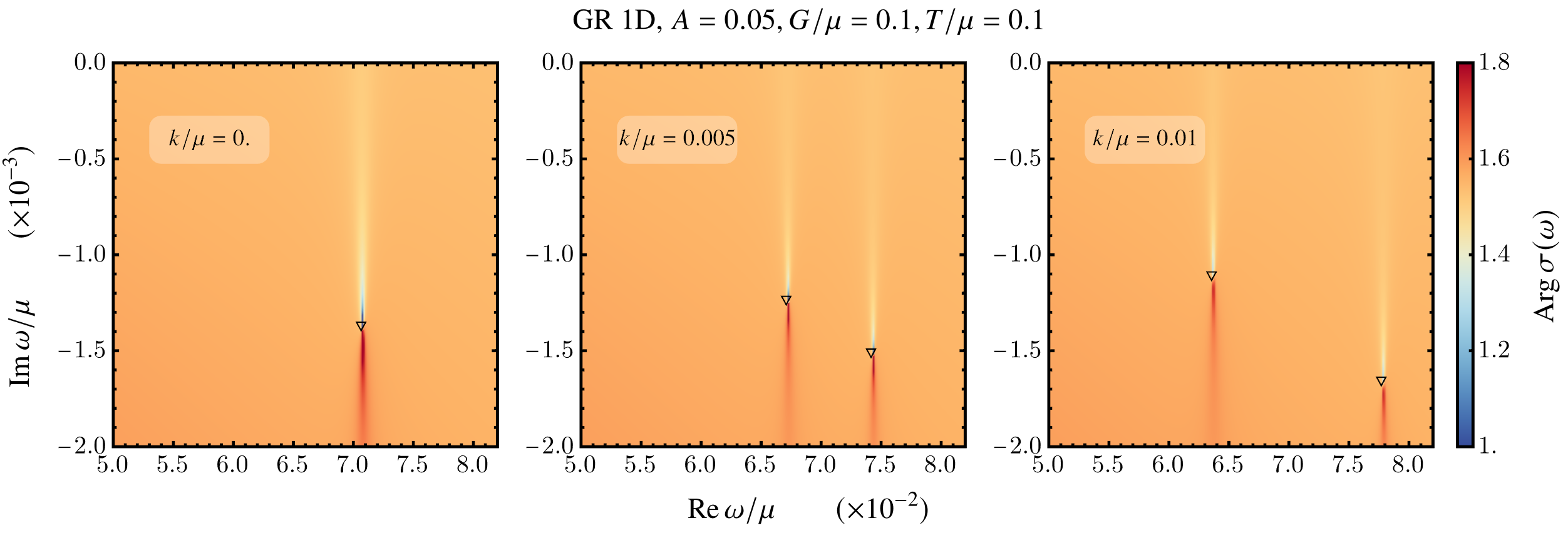
We will use the longitudinal optical conductivity as a probe. Generically this current will receive contributions from all hydrodynamic fluctuations; these essentially determine the low frequency long-wavelength response. At finite , this means we should see all modes described in (). At , however, the current is part of the sector and we will only see the first sector with its modes. Fig. 1 gives a schematic sketch of what the spectrum of the current-current correlator — and therefore the optical conductivity — should look like in the complex frequency plane based on our hydrodynamic predictions.
Precisely this expectation is reproduced by the numerical results in holographic duals to RN and GR black holes where hydrodynamics is emergent. Fig. 2 plots the density of the absolute value and argument of the optical conductivity for small values of the real part of the frequencies, i.e., zoomed in near the imaginary frequency axis. Each picture is at a different value of . We see that for there are only two purely diffusive poles, as predicted, that split into two propagating and two diffusive poles at finite . For finite , there should also be a third diffusive pole very close to the real axis. Its weight is very low, however, but it can be unveiled by zooming in carefully. This was plotted in Fig. 3 for (this choice of momenta proved more convenient to display). In all cases the location of these poles can be compared with the predictions from our hydrodynamical analysis after substituting in the relevant equation of state. The match is perfect for both and finite as denoted by the white circles in Fig. 2 and the triangles in Fig. 3. Similarly, we plotted in Fig. 4 the argument of the optical conductivity near the sound poles at momenta . The weight of these poles is very small and they are therefore difficult to identify in . The argument of , on the other hand, displays a jump at the poles. A similar analysis holds for the conjugate pair of poles at . These sound poles give rise to a characteristic peak in the real conductivity, first noted in [36, 37, 38].


To illustrate in more detail the hydrodynamical origin of all these poles and their full explanation in terms of thermodynamic quantities, one can track the location of the poles as a function of temperature. Focusing only on the purely diffusive poles (two for , and three for ), as they are more easily extracted numerically by scanning carefully over the negative imaginary frequency axis, we also find here a perfect match between numerics and hydrodynamic prediction, Eqs. () and () respectively, but now as function of ; see Fig. 5 and Fig. 6.
With our computational RN and GR examples we can also illustrate the subtle nature of the limit. As we saw in the previous section, the naive extrapolation to of the two sound modes does not correspond with the physical Drude pole and its equivalent . To emphasize this once more, the origin of this difference comes from the non-commutativity of the and limits. In Fig. 7, we have carefully analyzed the low regime of the GR black hole. For , the two diffusive poles are close to their values () and (). As we increase , they get closer and collide, leading to the two sound modes of (). This diffusion-to-sound crossover happens when illustrating the non-commuting limits , which means we can estimate the characteristic length scale of the interactions to be (see footnote 11).
Finally, to re-emphasize the underlying Bloch wave Umklapp physics, Fig. 8 shows the real part of the momentum-dependent optical conductivity in the plane. The right-hand plot is a zoomed-in version of the left-hand plot near the edge of the Brillouin zone . The gray dots are numerically obtained solutions of for the same parameters, showing that the hydrodynamic description of the matrix (3.1.2) at order matches the data over the entire Brillouin zone. At low frequency, we see the expected sound mode dominating the low frequency regime, but we also can see its interaction with the sound mode . They meet at the edge of the Brillouin zone and in the right-hand plot, we see the traditional level repulsion of Umklapp and the opening of a gap in the sound mode spectrum.


5 Conclusion
The crucial message of this paper is that hydrodynamic fluctuations in a periodically modulated background should be understood based on a Bloch wave analysis instead of simple plane waves. If the typical length scale of this modulation is sufficiently large and the amplitude sufficiently small, we can still use hydrodynamics to study the long-time response of the conserved charges. This is an old observation in neutral hydrodynamics, but deserves restudy for charged hydrodynamics given the novel experimental progress of observed hydrodynamic flow in electronic condensed matter systems [7, 8, 9]. This is particularly so in the presence of a charged fluid, which introduces an additional intrinsic diffusive mode. The presence of a spatial periodic modulation introduces Brillouin zone copies, also for this additional mode, and due to Umklapp at the Brillouin zone boundary this higher Bloch mode mixes with the long distance late time sound modes.
We showed how one can compute the explicit pattern and strengths of these mixings from the underlying hydrodynamics. As is standard but ever so useful in hydrodynamics is that the behavior of both the patterns and the strengths can be expressed in underlying thermodynamic quantities, notably the susceptibilities, combined with the transport coefficients.
An important feature of a periodic modulation — well known in the condensed matter physics context — is that it breaks translational symmetry. For a perturbatively small lattice the correction to the momentum pole can be interpreted as the momentum relaxation rate and our result agrees with the relaxation rate obtained through the memory matrix formalism, as it should. It is important to emphasize once more that even though there is one relaxation rate, this relaxation rate has two contributions and corresponding to the two longitudinal diffusive processes. A priori these can have different scaling in temperature.1414 14 This is the case in RN where and while in GR, they both scale with temperature with . They also exhibit different scaling in the lattice wavevector . Due to this, in systems with charge disorder parametrized as an averaging over many independent lattices, one of these terms will dominate. It is rather the other aspect of the periodic modulation — the presence of Bloch modes in higher Brillouin zones that we wish to emphasize here. At finite density this includes an Umklapped charge diffusion mode. As we analyzed in a companion paper, this mode may be of relevance in condensed matter physics [10]. The strange metal phase of high superconductors shows the development of a mysterious mid IR peak in the optical conductivity at temperatures ; see e.g. [39, 40]. The phenomenology of this peak is almost exactly reproduced by a collision between the Drude pole and the Umklapped charge diffusion pole in a holographic model of the strange metal dual to the Gubser Rocha black hole [10]. If it can be experimentally verified that charge transport in the strange metal is in fact hydrodynamical, this will be the explanation of that phenomenon.
Finally, we verified our results by numerically computing response functions in strongly coupled systems holographically dual to Reissner-Nordström and Gubser-Rocha black holes. The important feature is that hydrodynamics emerges naturally in holographic systems and is not an input. In the computed optical conductivities, we found precisely the poles matching those predicted by our hydrodynamics computation. As as function of varying parameters such as momentum and lattice strength, these poles show complicated behavior including pole collisions and level repulsion denoting various regime changes.
We conclude with emphasizing that the hydrodynamics description of those holographic systems remains valid throughout these collisions and level repulsions. This contrasts with recent studies on the validity of hydrodynamics postulated as a pole collision/level repulsion with a first UV (gapped) pole [41, 42, 43]. Our result here shows that this identification has to be done with care. The Umklapped modes are also a priori gapped modes in the zero momentum limit . However, they remain modes of the conserved charges, can be fully captured in a hydrodynamic description and play a different role from non-hydrodynamic UV modes.
The analysis carried in this paper crucially relied on a static background charge distribution to mimick the effects of a frozen ionic lattice. This ignores the effect of lattice vibrations. Including phonon modes would require a different setup. Moreover, the assumption of local thermal equilibrium rather strongly constrains the hierarchy of scales as . While the results we have achieved are rather general and only rely on the presence of global symmetries and periodicity – which would seem to imply this is valid for a wide range of metallic systems – one must remain cautious as to whether such hierarchy of scales is realized within physical systems.
Acknowledgements
We are very grateful to F. Balm and J. Zaanen for collaboration in the early stages of this project. We also thank D. Brattan, B. Goutéraux, K. Grosvenor, V. Ziogas and especially A. Krikun for discussions during the Nordita scientific program ”Recent developments in strongly correlated quantum matter”. This research was supported in part by the FOM program 167 (Strange Metals), by the Dutch Research Council (NWO) project 680-91-116 (Planckian Dissipation and Quantum Thermalisation: From Black Hole Answers to Strange Metal Questions.), and by the Dutch Research Council/Ministry of Education. The numerical computations were carried out on the Dutch national Cartesius and Snellius national supercomputing facilities with the support of the SURF Cooperative as well as on the ALICE-cluster of Leiden University. We are grateful for their help.
References
- [1] L. Brillouin, Wave Propagation in Periodic Structures: Electric Filters and Crystal Lattices, Dover Books on Engineering and Engineering Physics. McGraw-Hill Book Company, Incorporated (1946).
- [2] C. Elachi, Waves in active and passive periodic structures: A review, Proceedings of the IEEE 64(12), 1666 (1976), 10.1109/PROC.1976.10409.
- [3] L. Schächter, Beam-Wave Interaction in Periodic and Quasi-Periodic Structures, Particle Acceleration and Detection. Springer Berlin Heidelberg, ISBN 978-3-662-03398-2 (2013).
- [4] N. Jiménez, O. Umnova and J.-P. Groby, eds., Acoustic Waves in Periodic Structures, Metamaterials, and Porous Media, Springer International Publishing, 10.1007/978-3-030-84300-7 (2021).
- [5] A. Lucas and S. Sachdev, Memory matrix theory of magnetotransport in strange metals, Physical Review B 91(19), 195122 (2015), 10.1103/PhysRevB.91.195122, arXiv:1502.04704.
- [6] A. Lucas, Hydrodynamic transport in strongly coupled disordered quantum field theories, New Journal of Physics 17(11), 113007 (2015), 10.1088/1367-2630/17/11/113007, arXiv:1506.02662.
- [7] A. Lucas and K. C. Fong, Hydrodynamics of electrons in graphene, J. Phys. Condens. Matter 30(5), 053001 (2018), 10.1088/1361-648X/aaa274, arXiv:1710.08425.
- [8] A. Aharon-Steinberg, T. Völkl, A. Kaplan, A. K. Pariari, I. Roy, T. Holder, Y. Wolf, A. Y. Meltzer, Y. Myasoedov, M. E. Huber, B. Yan, G. Falkovich et al., Direct observation of vortices in an electron fluid, Nature 607(7917), 74 (2022), 10.1038/s41586-022-04794-y, arXiv:2202.02798.
- [9] L. Fritz and T. Scaffidi, Hydrodynamic electronic transport, 10.48550/arXiv.2303.14205 (2023), arXiv:2303.14205.
- [10] F. Balm, N. Chagnet, S. Arend, J. Aretz, K. Grosvenor, M. Janse, O. Moors, J. Post, V. Ohanesjan, D. Rodriguez-Fernandez, K. Schalm and J. Zaanen, T-linear resistivity, optical conductivity and Planckian transport for a holographic local quantum critical metal in a periodic potential, 10.48550/arXiv.2211.05492 (2022), arXiv:2211.05492.
- [11] V. Scopelliti, K. Schalm and A. Lucas, Hydrodynamic charge and heat transport on inhomogeneous curved spaces, Physical Review B 96(7), 075150 (2017), 10.1103/PhysRevB.96.075150, arXiv:1705.04325.
- [12] K. Jensen, M. Kaminski, P. Kovtun, R. Meyer, A. Ritz and A. Yarom, Parity-Violating Hydrodynamics in 2+1 Dimensions, JHEP 05, 102 (2012), 10.1007/JHEP05(2012)102, 1112.4498.
- [13] K. Pongsangangan, T. Ludwig, H. T. C. Stoof and L. Fritz, Hydrodynamics of charged two-dimensional Dirac systems II: The role of collective modes, 10.48550/arXiv.2206.09694 (2022), arXiv:2206.09694.
- [14] K. Pongsangangan, T. Ludwig, H. T. C. Stoof and L. Fritz, Hydrodynamics of charged two-dimensional Dirac systems I: Thermo-electric transport, Physical Review B 106(20), 205126 (2022), 10.1103/PhysRevB.106.205126, arXiv:2206.09687.
- [15] L. P. Kadanoff and P. C. Martin, Hydrodynamic equations and correlation functions, Annals of Physics 24, 419 (1963).
- [16] P. Kovtun, Lectures on hydrodynamic fluctuations in relativistic theories, J. Phys. A 45, 473001 (2012), 10.1088/1751-8113/45/47/473001, arXiv:1205.5040.
- [17] L. V. Delacrétaz, B. Goutéraux and V. Ziogas, Damping of Pseudo-Goldstone Fields, Physical Review Letters 128(14), 141601 (2022), 10.1103/PhysRevLett.128.141601, arXiv:2111.13459.
- [18] J. Armas, A. Jain and R. Lier, Approximate symmetries, pseudo-Goldstones, and the second law of thermodynamics, 10.48550/arXiv.2112.14373 (2022), arXiv:2112.14373.
- [19] D. Forster, Hydrodynamic Fluctuations, Broken Symmetry, and Correlation Functions, CRC Press, 10.1201/9780429493683 (2018).
- [20] S. A. Hartnoll and D. M. Hofman, Locally Critical Resistivities from Umklapp Scattering, Phys. Rev. Lett. 108, 241601 (2012), 10.1103/PhysRevLett.108.241601, arXiv:1201.3917.
- [21] R. A. Davison, K. Schalm and J. Zaanen, Holographic duality and the resistivity of strange metals, Phys. Rev. B 89(24), 245116 (2014), 10.1103/PhysRevB.89.245116, arXiv:1311.2451.
- [22] A. Donos, J. P. Gauntlett and V. Ziogas, Diffusion in inhomogeneous media, Phys. Rev. D 96(12), 125003 (2017), 10.1103/PhysRevD.96.125003, arXiv:1708.05412.
- [23] T. Andrade and A. Krikun, Commensurate lock-in in holographic non-homogeneous lattices, JHEP 03, 168 (2017), 10.1007/JHEP03(2017)168, 1701.04625.
- [24] M. Ammon and J. Erdmenger, Gauge/Gravity Duality: Foundations and Applications, Cambridge University Press, Cambridge, ISBN 978-1-107-01034-5, 10.1017/CBO9780511846373 (2015).
- [25] J. Casalderrey-Solana, H. Liu, D. Mateos, K. Rajagopal and U. A. Wiedemann, Gauge/String Duality, Hot QCD and Heavy Ion Collisions, Cambridge University Press, Cambridge, ISBN 978-1-107-02246-1, 10.1017/CBO9781139136747 (2014).
- [26] J. Zaanen, Y. Liu, Y.-W. Sun and K. Schalm, Holographic Duality in Condensed Matter Physics, Cambridge University Press, Cambridge, ISBN 978-1-107-08008-9, 10.1017/CBO9781139942492 (2015).
- [27] S. A. Hartnoll, A. Lucas and S. Sachdev, Holographic quantum matter, 10.48550/arXiv.1612.07324 (2018), arXiv:1612.07324.
- [28] S. Bhattacharyya, V. E. Hubeny, S. Minwalla and M. Rangamani, Nonlinear Fluid Dynamics from Gravity, Journal of High Energy Physics 2008(02), 045 (2008), 10.1088/1126-6708/2008/02/045, arXiv:0712.2456.
- [29] P. K. Kovtun and A. O. Starinets, Quasinormal modes and holography, Phys. Rev. D 72, 086009 (2005), 10.1103/PhysRevD.72.086009, arXiv:hep-th/0506184.
- [30] M. Edalati, J. I. Jottar and R. G. Leigh, Shear Modes, Criticality and Extremal Black Holes, JHEP 04, 075 (2010), 10.1007/JHEP04(2010)075, arXiv:1001.0779.
- [31] M. Edalati, J. I. Jottar and R. G. Leigh, Holography and the sound of criticality, JHEP 10, 058 (2010), 10.1007/JHEP10(2010)058, arXiv:1005.4075.
- [32] D. K. Brattan and S. A. Gentle, Shear channel correlators from hot charged black holes, JHEP 04, 082 (2011), 10.1007/JHEP04(2011)082, arXiv:1012.1280.
- [33] R. A. Davison and A. Parnachev, Hydrodynamics of cold holographic matter, JHEP 06, 100 (2013), 10.1007/JHEP06(2013)100, arXiv:1303.6334.
- [34] S. S. Gubser and F. D. Rocha, Peculiar properties of a charged dilatonic black hole in , Phys. Rev. D 81, 046001 (2010), 10.1103/PhysRevD.81.046001, arXiv:0911.2898.
- [35] N. Chagnet, F. Balm and K. Schalm, Quantization and variational problem of the Gubser-Rocha Einstein-Maxwell-Dilaton model, conformal and non-conformal deformations, and its proper thermodynamics, JHEP 03, 081 (2023), 10.1007/JHEP03(2023)081, arXiv:2209.13951.
- [36] G. T. Horowitz, J. E. Santos and D. Tong, Further Evidence for Lattice-Induced Scaling, Journal of High Energy Physics 2012(11), 102 (2012), 10.1007/JHEP11(2012)102, arXiv:1209.1098.
- [37] Y. Ling, C. Niu, J.-P. Wu and Z.-Y. Xian, Holographic Lattice in Einstein-Maxwell-Dilaton Gravity, Journal of High Energy Physics 2013(11), 6 (2013), 10.1007/JHEP11(2013)006, arXiv:1309.4580.
- [38] A. Donos and J. P. Gauntlett, The thermoelectric properties of inhomogeneous holographic lattices, Journal of High Energy Physics 2015(1), 35 (2015), 10.1007/JHEP01(2015)035, arXiv:1409.6875.
- [39] J. Hwang, T. Timusk and G. Gu, Doping dependent optical properties of bi2sr2cacu2o8+ , Journal of Physics: Condensed Matter 19(12), 125208 (2007).
- [40] L. V. Delacrétaz, B. Goutéraux, S. A. Hartnoll and A. Karlsson, Bad Metals from Fluctuating Density Waves, SciPost Physics 3(3), 025 (2017), 10.21468/SciPostPhys.3.3.025, 1612.04381.
- [41] D. Arean, R. A. Davison, B. Goutéraux and K. Suzuki, Hydrodynamic Diffusion and Its Breakdown near AdS2 Quantum Critical Points, Phys. Rev. X 11(3), 031024 (2021), 10.1103/PhysRevX.11.031024, arXiv:2011.12301.
- [42] N. Abbasi and S. Tahery, Complexified quasinormal modes and the pole-skipping in a holographic system at finite chemical potential, Journal of High Energy Physics 2020(10), 76 (2020), 10.1007/JHEP10(2020)076, arXiv:2007.10024.
- [43] N. Abbasi, M. Kaminski and O. Tavakol, Ultraviolet-regulated theory of non-linear diffusion, 10.48550/arXiv.2212.11499 (2022), arXiv:2212.11499.
- [44] P. Kovtun, D. T. Son and A. O. Starinets, Viscosity in strongly interacting quantum field theories from black hole physics, Phys. Rev. Lett. 94, 111601 (2005), 10.1103/PhysRevLett.94.111601, arXiv:hep-th/0405231.
- [45] R. A. Davison, B. Goutéraux and S. A. Hartnoll, Incoherent transport in clean quantum critical metals, JHEP 10, 112 (2015), 10.1007/JHEP10(2015)112, arXiv:1507.07137.
- [46] F. Balm, Florisbalm/hololattices, 10.5281/zenodo.7284816 (2022).
Appendix A Thermodynamics and susceptibilities
In this section of the supplementary material, we will briefly review some key thermodynamic identities related to the static susceptibilities. We will be interested in the conserved charges and their associated sources . Since we will be focusing on thermodynamics, we will only be interested in the equilibrium solution and therefore we will drop the notation for background thermodynamics quantities. As a reminder, the susceptibility matrix in the sector is defined as
| (55) |
while the momentum susceptibility is . Furthermore, we have the thermodynamic identity
| (56a) | ||||
| (56b) | ||||
| (56c) | ||||
such that . Using this relation and the first law , we have
| (57a) | ||||
| (57b) | ||||
Looking back at (55), this means that .
Appendix B Onsager relations
One of the important checks we must make that our dynamical system is well-defined is that it respects Onsager’s relations. These can be derived by considering how the system behaves under time-reversal invariance. Given the anti-unitary operator such that , we can classify each of the operators associated to our hydrodynamical variables by their representation under this operator. For a given operator , we will have with . Denoting the retarded Green’s function associated to a dynamical matrix by , we have
| (60) |
We can then see that, due to the anti-unitarity of ,
| (61) |
In Fourier space, this means and specifically for our periodic background, we can write the Green’s function as [22]
| (62) |
where we have used that the discrete lattice symmetry implies that . For this decomposition, the Onsager relation becomes
| (63a) | ||||
| (63b) | ||||
| (63c) | ||||
| (63d) | ||||
In the previous expression, we have introduced the diagonal matrix of eigenvalues and the notation . It is easy to check that for our background, and therefore since , we also have . We can write this relation in terms of the matrix of couplings
| (64) |
The elements of are simply the coefficients of the equations (6) written in terms of the sources and expanded in the basis (34). By using that , the relation (63) can then be written as
| (65) |
Let us apply this to the conservation equations (12) for an in-going momentum and an outgoing momentum
| (66a) | ||||
| (66b) | ||||
| (66c) | ||||
| (66d) | ||||
| (66e) | ||||
| (66f) | ||||
We now want to check the Onsager condition for using that . This can be done as follows for the sub-sector
| (67a) | ||||
| (67b) | ||||
| (67c) | ||||
| (67d) | ||||
while for the momentum-charge sector, we have
| (68a) | ||||
| (68b) | ||||
Finally, we only have to check the energy-momentum sector
| (69a) | ||||
| (69b) | ||||
We see therefore that the Onsager reciprocal relations are obeyed by our equations (12).
Appendix C Second order corrections in lattice strength
Let us consider here a dynamical matrix of size . The modes of this matrix are given by the solutions to the polynomial equation , where we can write
| (70) |
Suppose the coefficients have a power series expansion in a parameter . We are now interested in perturbative solutions , around a given solution . To do so we can define auxiliary polynomials such that
| (71) |
We can now expand the equation in at leading and subleading orders, and we find the following two conditions
| (72) |
The first equation is simply the leading order of the mode when there is no lattice while the second equation gives us the subleading correction. Finally, all the coefficients are themselves polynomials in which can be further expanded in order to get the corrections at higher order in momentum.1515 15 Note that in this method, the order of limits is chosen such that at finite , we would be getting the branch of solutions.
So far, it was implicitly assumed that the modes have no degeneracy when as that would imply that . When that happens, the correction is given by higher order terms with
| (73) |
This is the case for with . However, it turns out that for this matrix, and , so the two degenerate poles remain degenerate at this order in perturbation theory, with . A simpler way to see this is also to notice that the first line of is proportional to and therefore so will be . Consequently, this sector admits an exact conservation mode and we can use our non-degenerate method on the lower-right sub-block of this matrix where there is no degeneracy left. We would then see that the other pole also remains unshifted .
All that is therefore needed to compute the corrections in () and () is to know the coefficients for a given matrix . In the case of , we have
| (74a) | ||||
| (74b) | ||||
| (74c) | ||||
| (74d) | ||||
| (74e) | ||||
| (74f) | ||||
| (74g) | ||||
| (74h) | ||||
| (74i) | ||||
| (74j) | ||||
| (74k) | ||||
| (74l) | ||||
| (74m) | ||||
On the other hand, for the lower-right sub-block of the matrix , we find the following coefficients for the determinant
| (75a) | ||||
| (75b) | ||||
| (75c) | ||||
| (75d) | ||||
| (75e) | ||||
| (75f) | ||||
| (75g) | ||||
| (75h) | ||||
| (75i) | ||||
| (75j) | ||||
| (75k) | ||||
| (75l) | ||||
| (75m) | ||||
| (75n) | ||||
| (75o) | ||||
| (75p) | ||||
| (75q) | ||||
| (75r) | ||||
The coefficients for the determinant of the full longitudinal matrix () are too involved to be written down here but can be obtained in the exact same way. All these corrections were derived using Mathematica.
Appendix D Numerical computations in strongly coupled field theories dual to Reissner-Nordström and Gubser-Rocha AdS black holes: set-up
D.1 Thermodynamics
In Sec. 4, we focused on the specific conformal hydrodynamics that emerges at long wavelength and low frequencies from the holographic dynamics of the RN and GR black holes. In equilibrium the thermodynamic equation of state of each is given by (52) and (53) respectively. From these, we can determine the charge density as well as the entropy density while the energy density just follows from conformal invariance and is given by . One can further compute the various susceptibilities appearing in the hydrodynamics expressions of Sec. 3. As a reminder from Appendix A, the conformal equation of state also imposes and . For the RN black hole, the various susceptibilities and thermodynamic quantities are
| (76a) | ||||
| (76b) | ||||
| (76c) | ||||
| (76d) | ||||
| (76e) | ||||
| (76f) | ||||
| (76g) | ||||
| (76h) | ||||
while for the GR black hole we have
| (77a) | ||||
| (77b) | ||||
| (77c) | ||||
| (77d) | ||||
| (77e) | ||||
Lastly, we need to know some information on the transport coefficients and to compute the hydrodynamic response. These can be determined in the momentum-dependent homogeneous systems through and. In the case of conformal-to-AdS2 solutions like the RN and GR black holes, these expressions can be solved analytically for the two transport coefficients. The shear viscosity saturates the minimal viscosity bound [44] while was computed for a wide class of scaling black hole solutions [45] and here is given by
| (78a) | ||||
| (78b) | ||||
D.2 Numerics
We briefly review here how we compute the optical conductivity in the 2+1 dimensional strongly coupled conformal field theory holographically dual to the RN and GR black holes in the presence of a lattice. More details about the numerical methods used to compute these backgrounds and fluctuations can be found in the companion article [10]. The homogeneous RN black hole is a saddle point of the Einstein-Maxwell action
| (79) |
with metric
| (80) |
where is the emblackening factor and a U(1) gauge field. In the above expressions, is the radial coordinate ranging from the AdS boundary at to the horizon of the black hole at . The temperature of this black hole is .1616 16 A priori, if we allowed the black hole horizon to be arbitrarily located at , the temperature and chemical potential would be two independent parameters. However, when using the freedom to rescale the radial coordinate such that , we have implicitly fixed the temperature as a function of the chemical potential such that the only thermodynamic degree of freedom here is .
The GR black hole is similarly obtained by extremizing the Einstein-Maxwell-Dilaton action
| (81) |
with the potentials and Its metric is
| (82a) | ||||
| (82b) | ||||
The functions and are given by
| (83) |
This model is similar to the Einstein-Maxwell model with the addition of a neutral scalar field which controls the strength of the charge through the potential . A consequence of this is the ability to discharge some of the black hole charge near the horizon such that the extremal solution of this GR black hole will have a vanishing horizon and therefore vanishing entropy . The distance from extremality is controlled by the parameter : it is related to the chemical potential through and the temperature of the non-extremal black hole is given by .
To obtain backgrounds with an explicit lattice, we will allow for a more general ansatz
| (84a) | ||||
| (84b) | ||||
| (84c) | ||||
for RN with unchanged from (80) and
| (85a) | ||||
| (85b) | ||||
| (85c) | ||||
for GR with and unchanged from (82), but every field is now a priori a function of and . We require these fields to be regular near the horizon1717 17 One of the regularity conditions near the horizon is that . This choice has the direct consequence that the temperature of the black hole remains constant and given by the homogeneous value for each model. and that their UV behaviour at recovers AdS asymptotics.1818 18 In the case of the dilaton , the UV boundary condition chosen is a multi-trace deformation chosen such that the deformation is marginal and the boundary remains conformal. For more details, see [35]. Moreover, to encode the modulation of the chemical potential, we must impose the following boundary condition on the gauge field
| (86) |
The system is then solved numerically for the unknown functions .
To compute the optical conductivity in the holographically dual field theory, we must consider small fluctuations on top of this spatially modulated background. We linearize the Einstein equations around our lattice background
| (87a) | ||||
| (87b) | ||||
| (87c) | ||||
and solve for these fluctuations with infalling boundary conditions, corresponding to choosing the response sourced through the retarded Green’s function. The response in the radial electric field in answer to an oscillating source in the potential keeping the other components sourceless1919 19 Note that the condition for the dilaton to be sourceless is non-trivial and inherited from the mixed boundary condition of the background dilaton (see footnote 18). evaluated in the limit then translates through the holographic AdS/CFT correspondence into the longitudinal optical conductivity . In the language of our hydrodynamic setup in Sec. 2, this is akin to simply turning on an external electric field with momentum and frequency . This response is also solved for numerically.
The numerical solutions to these equations were obtained using a publicly available custom package [46] and computed on the Dutch national Cartesius and Snellius supercomputers with the support of SURF Cooperative.