Reconfigurable Electromagnetic Environments: A General FrameworkD. Dardari is with the Dipartimento di Ingegneria dell’Energia Elettrica e dell’Informazione “Guglielmo Marconi” (DEI), WiLAB-CNIT, University of Bologna, Cesena Campus, Cesena (FC), Italy, (e-mail: davide.dardari@unibo.it).

Davide Dardari

Abstract

The recent introduction of the SRE paradigm, enabled by RIS, has put in evidence the need for physically-consistent models and design tools for communication systems integrating EM (EM) and signal processing theories. In this perspective, starting from rigorous EM arguments, in this paper we propose a general framework for the characterization and design of programmable EM environments. We first show that any linear EM environment in the presence of boundary conditions can be interpreted as a space-variant linear feedback filter. Then we provide a methodology to characterize programmable EM systems as a linear graph described by matrix operators thus leading to the determination of the transfer function of the EM system. Finally, some examples are given related to the characterization and design of RIS, also showing that some previous results in the literature are just particular cases of our general framework.

Index Terms:

Smart Radio Environments; EM signal processing; Intelligent Surfaces; EM transfer function.

I Introduction

Recently, the SRE (SRE) concept has been introduced as one of the new design paradigms of next-generation networks [1, 2]. While in current communication systems the propagation environment is considered as given and the communicating devices are optimized to adapt to it, thanks to the deployment of programmable EM devices such as RIS (RIS), in SRE the environment enters into the design and optimization loop. This is expected to pave the way to more flexible wireless networks offering improved performance in terms of achievable rate, interference shaping, coverage extension, energy, and complexity reduction.

An extensive research activity has been devoted to the study of RIS-aided communication and localization systems, for example, the papers [3, 4, 5]. At the same time, the introduction of extremely electrically large antennas made of metasurfaces working at high frequency opened the door to the exploitation of the radiating near-field characteristics of the radio channel even at practical distances [6, 7, 3, 8, 9]. Despite the wide literature available today on the subject, the main shortcomings of previous studies are summarized in the following. On the one hand, oversimplified but tractable models, often relying on physically-inconsistent assumptions, have been mainly considered in system-level design and optimization that do not capture important peculiarities of the EMO composing the system. An example of a typically neglected EM phenomenon exhibited in smart surfaces is given by the Floquet modes, i.e., spurious reflections of surfaces characterized by a periodic impedance that might generate interference at non-desiderate angles and hence compromising the system performance [10]. Moreover, the search for the ultimate theoretical limits cannot rescind from an accurate description of the underlying EM phenomena [11, 12]. On the other hand, in the EM community, more emphasis has been put mainly on the characterization of single devices, often resorting to extensive EM-level simulations that can be barely included in a system-level analysis or real-time system optimization cycle [13, 14, 15, 16, 10, 17]. This dichotomy has made sense until now in a context where the EMO (for instance, the antenna) was seen as a “sensor” or “actuator/transducer” by the communication theorists community. In a near future, characterized by the presence of reconfigurable EM environments, the main objective will be the optimization of the system response, even in real-time, through the configuration of EMO’s parameters (e.g., the reflection properties of a metasurface-based RIS). This requires a holistic system view that calls for physically-consistent models and design tools integrating signal processing and EM theory [18]. Some recent works have undertaken this path. The investigation of the degrees of freedom of the wireless channel when using LIS, also dubbed as XL-MIMO or holographic MIMO, by modeling the surface as a continuous of infinitesimal antenna elements, has been conducted in [6, 7, 12, 3]. Regarding RIS, the work [19] proposes the modeling of a RIS as a set of elementary coupled dipoles and then characterizes its response in terms of impedance matrices. In [20], continuous and discrete models for the response of a perfect reflecting tile (i.e., a subset of the RIS) are derived starting from EM arguments and subsequently used in a two-step optimization approach targeted to achieving the desired communication quality by considering an ensemble of reconfigurable tiles. A recent survey that includes a critical discussion on RIS modeling can be found in [21].

Moving more at a system level, the authors in [22] define the concept of system EM transfer function in the wavenumber domain similarly to what is done in the signal processing community with the classical transfer function of a linear system in the frequency domain. This concept has been further elaborated in recent papers [23, 24, 4, 25]. In particular, [23] and [24] generalize the concept of EM transfer function for a stochastic Gaussian propagation environment characterized by rich scattering. Paper [25] derives the EM transfer function in the particular case of an infinite size surface with constant reflection coefficient by establishing a connection between the well-known image theorem in EM theory and the EM transfer function. Finally, a generalized expression of the EM field reflected by an EM skin in far-field and radiative near-field regimes is given in [26] and subsequently used to derive a unified method for the design of anomalous-reflecting and focusing EM skins. In [27], the same authors propose a numerical optimization problem for the design of SRE aiming at synthesizing a desired EM field distribution over a target region.

Previously mentioned studies are limited to the definition of the EM transfer function as a “black box” without providing any general methodology to compute it, apart from a few oversimplified scenarios or under oversimplified assumptions (e.g., no polarization, infinite uniform surfaces, point-wise scatterers, far-field regime). Moreover, none of the papers address the characterization of the EM transfer function for reconfigurable EMO such as RIS.

To fill the gap, in this paper we propose a general framework, starting from rigorous EM arguments valid both in far-field and (radiative and reactive) near-field regimes, aimed at giving a system-theoretic and physically-consistent interpretation of reconfigurable EM environments. It is shown that any system involving linear EMO can be described as a space-variant feedback system. Specifically, we show that boundary conditions applied to a generic EMO translate into a feedback system representation. Since the analysis and design of space-variant feedback systems are generally complex, inspired by mode-matching techniques, we propose an approach involving linear algebra operations over a graph that is useful to design and characterize EM systems in the presence of reconfigurable EMO. Subsequently, we derive the relationship between the EM transfer function and the linear algebra representation of the system, with particular emphasis on the characterization of smart surfaces. To illustrate the use of the proposed framework, some examples of the derivation of the EM transfer function are given. Some of them show that previous results in the literature can be seen as particular cases of our general framework. A final example is given targeted to the design of a RIS minimizing spurious interference caused by the presence of Floquet modes and/or other EM sources.

I-A Paper Organization

The rest of the paper is organized as follows: Sec. II formulates the problem of the description of a reconfigurable EM system composed of a certain number of EMO. In Secs. III, IV, and V, a linear algebra description of the EM system is developed through the introduction of harmonic basis functions (modes) (Sec. IV) and, subsequently, the derivation of the expressions for modes coupling (Sec. V), thus providing a graph-based interpretation of the system. The modeling and characterization of reconfigurable surfaces in terms of boundary conditions are addressed in Sec. VI. The relationship between the linear algebra description and the system EM transfer function is explained Sec. VII, where some examples are given for some particular cases of interest. Finally, in Sec. VIII the conclusions are drawn.

I-B Notation and Definitions

Lowercase bold variables denote vectors in the 3D space, i.e., ${\bf{r}}={\hat{\bf{x}}}\cdot r_{x}+{\hat{\bf{y}}}\cdot r_{y}+{\hat{\bf{z}}}\cdot r_{z}$ is a vector with cartesian coordinates $(r_{x},r_{y},r_{z})$ , $\hat{\bf{r}}$ is a unit vector denoting its direction, and $r=|{\bf{r}}|$ denotes its magnitude, where ${\hat{\bf{x}}}$ , ${\hat{\bf{y}}}$ , and ${\hat{\bf{z}}}$ represent the unit vectors in the $x$ , $y$ and $z$ directions, respectively. The cross product between vectors ${\bf{p}}$ and ${\bf{r}}$ is indicated with ${{\bf{p}}}\,{\scriptstyle\mathsf{x}}\,{{\bf{r}}}$ , whereas the scalar product with ${{\bf{p}}}\bm{\cdot}{{\bf{r}}}$ . $\delta(x)$ and $\delta_{n}$ represent, respectively, the Dirac delta pseudo-function and its discrete counterpart (Kronecker delta). Multi-variable versions can be defined as well, i.e., $\delta({\bf{r}})=\delta(x)\,\delta(y)\,\delta(z)$ and $\delta_{n,m}=\delta_{n-m}$ . Sans sherif capital letters (e.g., ${\mathsf{E}}({\bf{r}})$ , ${\mathsf{J}}({\bf{r}})$ ) represent EM vector functions (in the following named fields), whereas scalar functions are denoted with roman lowercase letters, i.e., $\phi({\bf{r}})$ . Boldface capital letters are matrices (e.g., ${\bf{A}}$ ), where ${\bf{I}}_{N}$ is the identity matrix of size $N$ , $\bm{0}_{N}$ the zero matrix of size $N$ , $a_{n,m}=[{\bf{A}}]_{n,m}$ represents the $(n,m)$ th element of matrix ${\bf{A}}$ , and ^∗ indicates the complex conjugate operator. $\nabla^{2}\,{\mathsf{E}}({\bf{r}})$ and $\nabla{\scriptstyle\mathsf{x}}\,{\mathsf{E}}({\bf{r}})$ are, respectively, the Laplacian and the curl of the vector function ${\mathsf{E}}({\bf{r}})$ . Surfaces, contours, and volumes are indicated with calligraphic letters $\mathcal{S}$ . Any linear transformation of a field $\mathsf{A}({\bf{r}})$ into a field $\mathsf{B}({\bf{r}})$ can be represented as $\mathsf{B}({\bf{r}})={\mathsf{{\underline{D}}}}\cdot\mathsf{A}({\bf{r}})$ , where ${\mathsf{{\underline{D}}}}$ is a dyadic that can be expressed as

{\mathsf{{\underline{D}}}}=\left(\begin{array}[]{ccc}{\mathsf{{{D}}}}^{(xx)}&{\mathsf{{{D}}}}^{(xy)}&{\mathsf{{{D}}}}^{(xz)}\\ {\mathsf{{{D}}}}^{(yx)}&{\mathsf{{{D}}}}^{(yy)}&{\mathsf{{{D}}}}^{(yz)}\\ {\mathsf{{{D}}}}^{(zx)}&{\mathsf{{{D}}}}^{(zy)}&{\mathsf{{{D}}}}^{(zz)}\\ \end{array}\right)\,.

Typically, ${\mathsf{{\underline{D}}}}$ depends on the position ${\bf{r}}$ even though this is not shown explicitly to lighten the notation. Often an operation involving a dyadic can be expressed in matrix form. Define $\text{Sinc}\left({x}\right)=\sin(\pi\,x)/(\pi\,x)$ for $x\neq 0$ , 1 for $x=0$ , and $\text{Rect}\left({x}\right)=1$ for $|x|<1/2$ , zero otherwise. Furthermore, denote by $\mu$ , $\epsilon$ , and $\eta=\sqrt{\mu/\epsilon}$ the free-space permittivity, permeability and impedance, respectively, and $c$ the speed of light.

Refer to caption — Fig. 1: General EM scenario with interacting EMO.

II Reconfigurable EM System

II-A Problem formulation

We consider $M$ linear time-invariant EMO are present in the system sketched in Fig. 1, and we indicate with $\mathcal{S}^{(m)}$ , $m=1,2,\ldots,M$ , the surface that encloses the $m$ th EMO. Each surface can represent the physical surface of the EMO or any arbitrary surface which encloses it. We work in the frequency domain, where time-harmonic excitations $\exp(\jmath\omega t)$ are assumed, being $\omega$ the angular frequency, and all fields and sources are phasors. Denote with ${\mathsf{J}}^{(m)}({\bf{r}})$ and ${\mathsf{M}}^{(m)}({\bf{r}})$ the electric and magnetic currents densities, respectively, on surface $\mathcal{S}^{(m)}$ .¹¹ 1 In general, $\mathcal{S}^{(m)}$ may be a surface or a contour (e.g., a wire antenna). With a little abuse of nomenclature, for further convenience, we will still denote it as surface. Notice that ${\mathsf{J}}^{(m)}({\bf{r}})$ and ${\mathsf{M}}^{(m)}({\bf{r}})$ are zero outside $\mathcal{S}^{(m)}$ . The total electric and magnetic currents present in the system are given by ${\mathsf{J}}({\bf{r}})=\sum_{m=1}^{M}{\mathsf{J}}^{(m)}({\bf{r}})$ and ${\mathsf{M}}({\bf{r}})=\sum_{m=1}^{M}{\mathsf{M}}^{(m)}({\bf{r}})$ , respectively. In general, ${\mathsf{J}}^{(m)}({\bf{r}})$ and ${\mathsf{M}}^{(m)}({\bf{r}})$ can be decomposed into the sum of the impressed $\left(\mathsf{J}_{\text{imp}}^{(m)}({\bf{r}})\,,\mathsf{M}_{\text{imp}}^{(m)}({\bf{r}})\right)$ (if any) and induced $\left(\mathsf{J}_{\text{s}}^{(m)}({\bf{r}})\,,\mathsf{M}_{\text{s}}^{(m)}({\bf{r}})\right)$ currents

\displaystyle{\mathsf{J}}^{(m)}({\bf{r}})

\displaystyle=\mathsf{J}_{\text{s}}^{(m)}({\bf{r}})+\mathsf{J}_{\text{imp}}^{(m)}({\bf{r}})

\displaystyle{\mathsf{M}}^{(m)}({\bf{r}})

\displaystyle=\mathsf{M}_{\text{s}}^{(m)}({\bf{r}})+\mathsf{M}_{\text{imp}}^{(m)}({\bf{r}})\,.

(1)

According to the equivalent principle [28], the introduction of (fictitious) induced currents, satisfying the boundary conditions at the corresponding surface, permits to consider the induced current sources to radiate into an unbounded space. Therefore, the EM field, i.e., the electric and magnetic fields, generated by all the currents present in the system at the generic location ${\bf{r}}$ can be computed under the free-space condition, that is,

\displaystyle\left(\begin{array}[]{c}{\mathsf{E}}({\bf{r}})\\ {\mathsf{H}}({\bf{r}})\\ \end{array}\right)=\left(\begin{array}[]{cc}{\mathsf{{\underline{G}}}_{\text{EJ}}}&{\mathsf{{\underline{G}}}_{\text{EM}}}\\ {\mathsf{{\underline{G}}}_{\text{HM}}}&{\mathsf{{\underline{G}}}_{\text{HJ}}}\\ \end{array}\right)\cdot\left(\begin{array}[]{c}{\mathsf{J}}({\bf{r}})\\ {\mathsf{M}}({\bf{r}})\\ \end{array}\right)={\mathsf{{\underline{G}}}}\cdot\left(\begin{array}[]{c}{\mathsf{J}}({\bf{r}})\\ {\mathsf{M}}({\bf{r}})\\ \end{array}\right)

where the above dyadics are given by [29]

$\displaystyle{\mathsf{{\underline{G}}}_{\text{EJ}}}\cdot{\mathsf{J}}({\bf{r}})$	$\displaystyle=\frac{1}{\jmath\omega\epsilon}\nabla{\scriptstyle\mathsf{x}}\,\nabla{\scriptstyle\mathsf{x}}\,\int_{\mathcal{S}}{G_{0}}({\bf{r}}-{\bf{s}})\,{\mathsf{J}}({\bf{s}})\,d{\bf{s}}$	(10)
$\displaystyle{\mathsf{{\underline{G}}}_{\text{EM}}}\cdot{\mathsf{M}}({\bf{r}})$	$\displaystyle=-\nabla{\scriptstyle\mathsf{x}}\,\int_{\mathcal{S}}{G_{0}}({\bf{r}}-{\bf{s}})\,{\mathsf{M}}({\bf{s}})\,d{\bf{s}}$	(11)
$\displaystyle{\mathsf{{\underline{G}}}_{\text{HJ}}}\cdot{\mathsf{J}}({\bf{r}})$	$\displaystyle=\nabla{\scriptstyle\mathsf{x}}\,\int_{\mathcal{S}}{G_{0}}({\bf{r}}-{\bf{s}})\,{\mathsf{J}}({\bf{s}})\,d{\bf{s}}$	(12)
$\displaystyle{\mathsf{{\underline{G}}}_{\text{HM}}}\cdot{\mathsf{M}}({\bf{r}})$	$\displaystyle=\frac{1}{\jmath\omega\mu}\nabla{\scriptstyle\mathsf{x}}\,\nabla{\scriptstyle\mathsf{x}}\,\int_{\mathcal{S}}{G_{0}}({\bf{r}}-{\bf{s}})\,{\mathsf{M}}({\bf{s}})\,d{\bf{s}}$	(13)

being $\mathcal{S}=\bigcup_{m=1}^{M}\mathcal{S}^{(m)}$ . The function

{G_{0}}({\bf{r}})=\frac{\exp(-\jmath k_{0}|{\bf{r}}|)}{4\pi|{\bf{r}}|}

(14)

is the free-space scalar Green function, where $k_{0}=2\pi/\lambda$ is the wavenumber and $\lambda=2\pi c/\omega$ is the wavelength. It can be easily noticed from the previous equations that the propagation phenomenon operates as a space-invariant linear filter because ${G_{0}}({\bf{r}})$ appears in (10)-(13) as a function of only the difference ${\bf{r}}-{\bf{s}}$ .

Define the EM field $\left(\mathsf{E}_{\text{t}}^{(m)}({\bf{r}})\,,\mathsf{H}_{\text{t}}^{(m)}({\bf{r}})\right)$ tangent to surface $\mathcal{S}^{(m)}$ of the $m$ th EMO. For any linear time-invariant EMO, the induced currents are linear functionals of the EM field tangent to the surface so that they can be described as follows (constitutive equation) [7]

\displaystyle\left(\begin{array}[]{c}\mathsf{J}_{\text{s}}^{(m)}({\bf{r}})\\ \mathsf{M}_{\text{s}}^{(m)}({\bf{r}})\\ \end{array}\right)=\left(\begin{array}[]{cc}{\mathsf{{\underline{D}}}_{\text{JE}}^{\,(m)}}&{\mathsf{{\underline{D}}}_{\text{JH}}^{\,(m)}}\\ {\mathsf{{\underline{D}}}_{\text{ME}}^{\,(m)}}&{\mathsf{{\underline{D}}}_{\text{MH}}^{\,(m)}}\\ \end{array}\right)\cdot\left(\begin{array}[]{c}\mathsf{E}_{\text{t}}^{(m)}({\bf{r}})\\ \mathsf{H}_{\text{t}}^{(m)}({\bf{r}})\\ \end{array}\right)={\mathsf{{\underline{D}}}^{\,(m)}}\cdot\left(\begin{array}[]{c}\mathsf{E}_{\text{t}}^{(m)}({\bf{r}})\\ \mathsf{H}_{\text{t}}^{(m)}({\bf{r}})\\ \end{array}\right)

where the dyadic ${\mathsf{{\underline{D}}}_{\text{JE}}^{\,(m)}}$ can be expressed in general as

\displaystyle{\mathsf{{\underline{D}}}_{\text{JE}}^{\,(m)}}\cdot\mathsf{E}_{\text{t}}^{(m)}({\bf{r}})

\displaystyle=\int_{\mathcal{S}^{(m)}}{\mathsf{{\underline{D}}}}_{\text{JE}}^{\,(m)}({\bf{r}},{\bf{s}})\,\mathsf{E}_{\text{t}}^{(m)}({\bf{s}})\,d{\bf{s}}

(23)

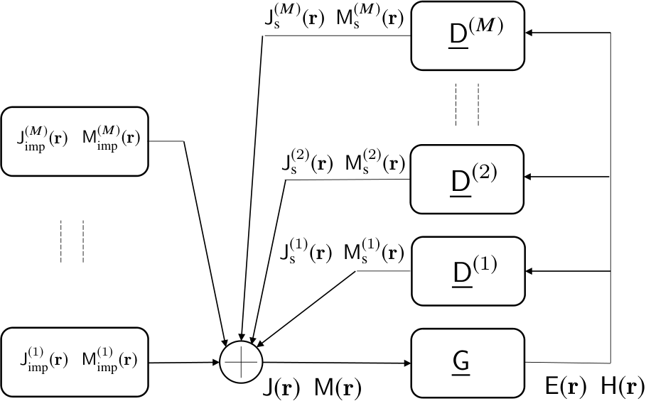
being ${\mathsf{{\underline{D}}}}_{\text{JE}}^{\,(m)}({\bf{r}},{\bf{s}})$ the impulse response dyadic describing completely the relationship between the electric field and the induced current at the $m$ th EMO. Similar expressions can be written for the dyadics ${\mathsf{{\underline{D}}}_{\text{JH}}^{\,(m)}}$ , ${\mathsf{{\underline{D}}}_{\text{ME}}^{\,(m)}}$ , and ${\mathsf{{\underline{D}}}_{\text{MH}}^{\,(m)}}$ . For instance, in non-magnetic scatterers, the induced magnetic current is zero, i.e., $\mathsf{M}_{\text{s}}^{(m)}({\bf{r}})=0$ , then ${\mathsf{{\underline{D}}}_{\text{ME}}^{\,(m)}}={\mathsf{{\underline{D}}}_{\text{MH}}^{\,(m)}}=0$ [30]. The particular form of ${\mathsf{{\underline{D}}}^{\,(m)}}$ depends on the model adopted for the EMO and the target level of accuracy. Some examples are provided in Sec. VII. The previous relationships can be represented in the scheme of Fig. 2 where it is evident that any EM scenario can be viewed as a feedback system in which the impressed currents represent the inputs, the propagation phenomenon ${\mathsf{{\underline{G}}}}$ is a space-invariant filter and each EMO can be seen as a space-variant filter (in analogy with time-variant filters) whose output consists of the induced currents. The above feedback system involves integral equations whose solution is, in general, a complex problem typically addressed numerically. In this paper, we introduce a methodology to bypass this problem.

II-B Wavenumber Domain Representation

For what follows, it is convenient to introduce the representation of the fields in the wavenumber domain ${\bm{\kappa}}=\kappa_{x}{\hat{\bf{x}}}+\kappa_{y}{\hat{\bf{y}}}+\kappa_{z}{\hat{\bf{z}}}$ through the 3D Fourier transform. Specifically, given a generic field $\mathsf{A}({\bf{r}})$ , we can write

\displaystyle\widetilde{\mathsf{A}}({\bm{\kappa}})

\displaystyle=\mathcal{F}\left[\mathsf{A}({\bf{r}})\right]=\int_{{\cal{R}}^{3}}\mathsf{A}({\bf{r}})\,e^{-\jmath\,{\bm{\kappa}}\bm{\cdot}{\bf{r}}}\,d{\bf{r}}

(24)

\displaystyle\mathsf{A}({\bf{r}})

\displaystyle=\mathcal{F}^{-1}\left[\widetilde{\mathsf{A}}({\bm{\kappa}})\right]=\frac{1}{(2\pi)^{3}}\int_{{\cal{R}}^{3}}\widetilde{\mathsf{A}}({\bm{\kappa}})\,e^{\jmath\,{\bm{\kappa}}\bm{\cdot}{\bf{r}}}\,d{\bm{\kappa}}\,.

(25)

When applied to the EM field, the inverse Fourier representation in (25) expresses the EM field in terms of mathematical plane waves [31]. By inspection of (25), the plane wave with wavenumber ${\bm{\kappa}}$ , travels in the positive $w$ -direction (forward wave), with $w\in\{x,y,z\}$ , when its component ${\bm{\kappa}}_{w}<0$ , whereas when ${\bm{\kappa}}_{w}>0$ the wave travels in the negative $w$ -direction (backward wave). It follows that

{\widetilde{G}_{0}}({\bm{\kappa}})=\mathcal{F}\left[{G_{0}}({\bf{r}})\right]=\frac{1}{|{\bm{\kappa}}|^{2}-k_{0}^{2}}\

(26)

and from (10)-(13), that

	$\displaystyle\widetilde{\mathsf{E}}({\bm{\kappa}})$	$\displaystyle=\mathcal{F}\left[{\mathsf{E}}({\bf{r}})\right]=\frac{\jmath\,{\widetilde{G}_{0}}({\bm{\kappa}})\,}{\omega\epsilon}{{\bm{\kappa}}}\,{\scriptstyle\mathsf{x}}\,{{{\bm{\kappa}}}\,{\scriptstyle\mathsf{x}}\,{{\widetilde{\mathsf{J}}}({\bm{\kappa}})}}-\jmath\,{\widetilde{G}_{0}}({\bm{\kappa}})\,{{\bm{\kappa}}}\,{\scriptstyle\mathsf{x}}\,{{\widetilde{\mathsf{M}}}({\bm{\kappa}})}=\jmath\,{\widetilde{G}_{0}}({\bm{\kappa}}){{\bm{\kappa}}}\,{\scriptstyle\mathsf{x}}\,{\left[\frac{\eta}{k_{0}}{{{\bm{\kappa}}}\,{\scriptstyle\mathsf{x}}\,{{\widetilde{\mathsf{J}}}({\bm{\kappa}})}}-{\widetilde{\mathsf{M}}}({\bm{\kappa}})\right]}$		(27)
	$\displaystyle\widetilde{\mathsf{H}}({\bm{\kappa}})$	$\displaystyle=\mathcal{F}\left[{\mathsf{H}}({\bf{r}})\right]=\frac{\jmath\,{\widetilde{G}_{0}}({\bm{\kappa}})\,}{\omega\mu}{{\bm{\kappa}}}\,{\scriptstyle\mathsf{x}}\,{{{\bm{\kappa}}}\,{\scriptstyle\mathsf{x}}\,{{\widetilde{\mathsf{M}}}({\bm{\kappa}})}}+\jmath\,{\widetilde{G}_{0}}({\bm{\kappa}})\,{{\bm{\kappa}}}\,{\scriptstyle\mathsf{x}}\,{{\widetilde{\mathsf{J}}}({\bm{\kappa}})}=\jmath\,{\widetilde{G}_{0}}({\bm{\kappa}})\,{{\bm{\kappa}}}\,{\scriptstyle\mathsf{x}}\,{\left[\frac{1}{k_{0}\,\eta}{{\bm{\kappa}}}\,{\scriptstyle\mathsf{x}}\,{{\widetilde{\mathsf{M}}}({\bm{\kappa}})}+{\widetilde{\mathsf{J}}}({\bm{\kappa}})\right]}$		(28)

where ${\widetilde{\mathsf{J}}}({\bm{\kappa}})=\mathcal{F}\left[{\mathsf{J}}({\bf{r}})\right]$ , ${\widetilde{\mathsf{M}}}({\bm{\kappa}})=\mathcal{F}\left[{\mathsf{M}}({\bf{r}})\right]$ , and we have considered that $\mathcal{F}\left[\nabla{\scriptstyle\mathsf{x}}\,\mathsf{A}\right]=\jmath\,{{\bm{\kappa}}}\,{\scriptstyle\mathsf{x}}\,{\widetilde{\mathsf{A}}({\bm{\kappa}})}$ .

The spatial filtering operated by the Green operator is evident in (26) which corresponds to a low-pass filter with a cut-off frequency equal to $k_{0}$ . This means that the EM field has a spatial low-pass characteristic. Incidentally, by defining ${\bm{\kappa}}_{{\bf{r}}}=k_{0}\,\hat{\bf{r}}$ , the EM field at location ${\bf{r}}$ in far-field conditions is proportional to the Fourier transform of the sources [28], that is,

	$\displaystyle{\mathsf{E}}({\bf{r}})$	$\displaystyle\simeq\jmath k_{0}\frac{e^{-\jmath\,k_{0}\,\|{\bf{r}}\|}}{4\pi\|{\bf{r}}\|}\,{\hat{\bf{r}}}\,{\scriptstyle\mathsf{x}}\,{\left[\eta\,{{\hat{\bf{r}}}\,{\scriptstyle\mathsf{x}}\,{{\widetilde{\mathsf{J}}}({\bm{\kappa}}_{{\bf{r}}})}}+{\widetilde{\mathsf{M}}}({\bm{\kappa}}_{{\bf{r}}})\right]}$
	$\displaystyle{\mathsf{H}}({\bf{r}})$	$\displaystyle\simeq\jmath k_{0}\frac{e^{-\jmath\,k_{0}\,\|{\bf{r}}\|}}{4\pi\|{\bf{r}}\|}\,{\hat{\bf{r}}}\,{\scriptstyle\mathsf{x}}\,{\left[\frac{1}{\eta}\,{{\hat{\bf{r}}}\,{\scriptstyle\mathsf{x}}\,{{\widetilde{\mathsf{M}}}({\bm{\kappa}}_{{\bf{r}}})}}-{\widetilde{\mathsf{J}}}({\bm{\kappa}}_{{\bf{r}}})\right]}\,.$		(29)

By applying the Fourier transform to (II-A) we obtain

\displaystyle{\widetilde{\mathsf{J}}}_{\text{s}}^{(m)}({\bm{\kappa}})=\frac{1}{(2\pi)^{3}}\int_{{\cal{R}}^{3}}\underline{\widetilde{\mathsf{D}}}_{\text{JE}}^{(m)}({\bm{\kappa}},\overline{{\bm{\kappa}}})\,\widetilde{\mathsf{E}}_{\text{t}}(\overline{{\bm{\kappa}}})\,d\overline{{\bm{\kappa}}}+\frac{1}{(2\pi)^{3}}\int_{{\cal{R}}^{3}}\underline{\widetilde{\mathsf{D}}}_{\text{JH}}^{(m)}({\bm{\kappa}},\overline{{\bm{\kappa}}})\,\widetilde{\mathsf{H}}_{\text{t}}(\overline{{\bm{\kappa}}})\,d\overline{{\bm{\kappa}}}

(30)

where $\underline{\widetilde{\mathsf{D}}}_{\text{JE}}^{(m)}({\bm{\kappa}},\overline{{\bm{\kappa}}})$ and $\underline{\widetilde{\mathsf{D}}}_{\text{JH}}^{(m)}({\bm{\kappa}},\overline{{\bm{\kappa}}})$ take the role of the bi-frequency system functions, or mapping functions, in analogy with the bi-frequency system function of time-variant systems [32]. They give the induced current response of the EMO at wavenumber ${\bm{\kappa}}$ when a plane wave with wavenumber $\overline{{\bm{\kappa}}}$ is applied at the input. Similar expressions hold for ${\widetilde{\mathsf{M}}}_{\text{s}}^{(m)}({\bm{\kappa}})$ . $\underline{\widetilde{\mathsf{D}}}_{\text{JE}}^{(m)}({\bm{\kappa}},\overline{{\bm{\kappa}}})$ , $\underline{\widetilde{\mathsf{D}}}_{\text{JH}}^{(m)}({\bm{\kappa}},\overline{{\bm{\kappa}}})$ , $\underline{\widetilde{\mathsf{D}}}_{\text{ME}}^{(m)}({\bm{\kappa}},\overline{{\bm{\kappa}}})$ , and $\underline{\widetilde{\mathsf{D}}}_{\text{MH}}^{(m)}({\bm{\kappa}},\overline{{\bm{\kappa}}})$ , depend on EMO’s characteristics and configuration and might represent the optimization objective in a reconfigurable EM system, as it will be shown in the next. Due to the presence of feedback, they impose the boundary conditions that are responsible for the presence of field discontinuity. This aspect will be discussed in Sec. VI.

II-C System EM Transfer Function

It is of interest to evaluate the (space-variant) system EM transfer function $\underline{\widetilde{\cal{H}}}({\bm{\kappa}},\overline{{\bm{\kappa}}})$ (or system Green function) that relates the impressed currents (input) and the resulting EM field (output). Typically, only the impressed electric currents and the electric field are considered then, without loss of generality, we focus on the EM transfer function component $\underline{\widetilde{\cal H}}_{\text{EJ}}({\bm{\kappa}},\overline{{\bm{\kappa}}})$ that relates ${\widetilde{\mathsf{J}}}_{\text{imp}}({\bm{\kappa}})=\sum_{m}{\widetilde{\mathsf{J}}}_{\text{imp}}^{(m)}({\bm{\kappa}})$ and the electric field $\widetilde{\mathsf{E}}({\bm{\kappa}})$ . In general, being the system space variant, $\widetilde{\mathsf{E}}({\bm{\kappa}})$ can be expressed as

\displaystyle\widetilde{\mathsf{E}}({\bm{\kappa}})=\frac{1}{(2\pi)^{3}}\int_{{\cal{R}}^{3}}\underline{\widetilde{\cal H}}_{\text{EJ}}({\bm{\kappa}},{\bf{k}})\,{\widetilde{\mathsf{J}}}_{\text{imp}}({\bf{k}})\,d{\bf{k}}\,.

(31)

The system transfer function $\underline{\widetilde{\cal H}}_{\text{EJ}}({\bm{\kappa}},\overline{{\bm{\kappa}}})$ indicates what is the response of the entire system at wavenumber ${\bm{\kappa}}$ when it is solicited by an impressed current with wavenumber $\overline{{\bm{\kappa}}}$ . Specifically, the component ${\widetilde{\cal H}}_{\text{EJ}}^{(xx)}({\bm{\kappa}},\overline{{\bm{\kappa}}})$ of dyadic $\underline{\widetilde{\cal H}}_{\text{EJ}}({\bm{\kappa}},\overline{{\bm{\kappa}}})$ represents the response of the system at polarization $\hat{\bf{a}}_{x}$ when solicited by the harmonic current ${\widetilde{\mathsf{J}}}_{\text{imp}}({\bm{\kappa}})=\hat{\bf{a}}_{x}(2\pi)^{3}\delta({\bm{\kappa}}-\overline{{\bm{\kappa}}})$ . Similarly for the other polarization combinations. The harmonic current is a dual of the infinitesimal source current, and it has only a mathematical meaning.

It is customary to evaluate the electric field observed along a plane, for instance, the $x-y$ plane at $z=z_{\text{o}}$ (not containing current sources), namely $\widetilde{\mathsf{E}}(\kappa_{x},\kappa_{y};z_{\text{o}})$ . For example, this could be the plane where a receiving antenna array or a surface is located. As a consequence, we can define the EM system transfer function or channel transfer function [22, 23, 24, 25], namely $\underline{{\widetilde{\mathcal{H}}}}(\kappa_{x},\kappa_{y},\overline{\kappa}_{x},\overline{\kappa}_{y};z_{\text{s}}\,,z_{\text{o}})$ , with reference to a source in the $x-y$ plane at $z=z_{\text{s}}$ , where the impressed (real or equivalent) currents ${\mathsf{J}_{\text{imp}}}(x,y;z_{\text{s}})$ are supposed to lay, and the $x-y$ observation plane at $z=z_{\text{o}}$ [22, 23, 24, 25]. It follows that

\displaystyle\widetilde{\mathsf{E}}(\kappa_{x},\kappa_{y};z_{\text{o}})

\displaystyle=\frac{1}{2\pi}\int\widetilde{\mathsf{E}}({\bm{\kappa}})\,e^{\jmath\kappa_{z}\,z_{\text{o}}}\,d\kappa_{z}=\int_{{\cal{R}}^{2}}\underline{{\widetilde{\mathcal{H}}}}(\kappa_{x},\kappa_{y},k_{x},k_{y};z_{\text{s}}\,,z_{\text{o}})\,{\widetilde{\mathsf{J}}}_{\text{imp}}(k_{x},k_{y};z_{\text{s}})\,dk_{x}\,dk_{y}

(32)

where

\displaystyle\underline{{\widetilde{\mathcal{H}}}}(\kappa_{x},\kappa_{y},\overline{\kappa}_{x},\overline{\kappa}_{y};z_{\text{s}}\,,z_{\text{o}})

\displaystyle=\frac{1}{(2\pi)^{2}}\int_{{\cal{R}}^{2}}\underline{\widetilde{\cal H}}_{\text{EJ}}({\bm{\kappa}},\overline{{\bm{\kappa}}})\,e^{-\jmath\kappa_{z}\,z_{\text{s}}}e^{\jmath\overline{\kappa}_{z}\,z_{\text{o}}}d\kappa_{z}\,\overline{\kappa}_{z}\,.

(33)

Analogously to $\underline{\widetilde{\cal H}}_{\text{EJ}}({\bm{\kappa}},\overline{{\bm{\kappa}}})$ , the component ${{\widetilde{\mathcal{H}}}}^{(xx)}(\kappa_{x},\kappa_{y},\overline{\kappa}_{x},\overline{\kappa}_{y};z_{\text{s}}\,,z_{\text{o}})$ of (33) gives the system response observed on the plane $z=z_{\text{o}}$ at the 2D wavenumber $(\kappa_{x},\kappa_{y})$ and polarization $\hat{\bf{a}}_{x}$ when solicited by the harmonic current ${\widetilde{\mathsf{J}}}_{\text{imp}}({\bm{\kappa}})=\hat{\bf{a}}_{x}(2\pi)^{2}\delta(\kappa_{x}-\overline{\kappa}_{x})\,\delta(\kappa_{y}-\overline{\kappa}_{y})\,e^{-\jmath\kappa_{z}z_{\text{s}}}$ located on the plane $z=z_{\text{s}}$ . Note that (33) is a vectorial transfer function, whereas the treatment in [22, 23, 24] consider scalar fields.

In the following, we present an approach, based on linear algebra, to compute efficiently the EM transfer function $\underline{\widetilde{\cal H}}_{\text{EJ}}({\bm{\kappa}},\overline{{\bm{\kappa}}})$ in (31) or $\underline{{\widetilde{\mathcal{H}}}}(\kappa_{x},\kappa_{y},\overline{\kappa}_{x},\overline{\kappa}_{y};z_{\text{s}}\,,z_{\text{o}})$ in (33), which allows to easily incorporate design, analysis, and optimization problems involving reconfigurable EMO. The approach permits also the evaluation of the EM field as well as the impressed currents on each EMO’s surface.

III Linear Algebra Formulation

The following approach takes inspiration from the well-known method of moments or mode matching [33]. For convenience, we introduce the inner product between vector functions $\mathsf{A}({\bf{r}})$ and $\mathsf{B}({\bf{r}})$ , defined on the generic surface $\mathcal{S}$ , as

\displaystyle\left<{\mathsf{A}({\bf{r}})}\,,{\mathsf{B}({\bf{r}})}\right>=\int_{\mathcal{S}}\mathsf{A}({\bf{r}})\bm{\cdot}\mathsf{B}^{*}({\bf{r}})\,d{\bf{r}}\,.

(34)

Note that his definition is different from that used in the method of moments [34]. Suppose $\left\{{\mathbf{\Phi}}^{(m)}_{n}({\bf{r}})\right\}_{n=1,2,\ldots,N^{(m)}}$ is a complete vector orthonormal basis set for $\mathcal{S}^{(m)}$ . The orthogonality condition implies that

\displaystyle\left<{{\mathbf{\Phi}}^{(m)}_{n}({\bf{r}})}\,,{{\mathbf{\Phi}}^{(m)}_{i}({\bf{r}})}\right>=\delta_{n,i}\,.

(35)

It is worth noticing that ${\mathbf{\Phi}}^{(m)}_{n}({\bf{r}})$ is a 3D vector which is tangent to the surface $\mathcal{S}^{(m)}$ for all ${\bf{r}}\in\mathcal{S}^{(m)}$ and zero otherwise. Moreover, all the basis sets refer to disjoint surfaces so that $\left<{\mathbf{\Phi}}^{(m)}_{u}({\bf{r}}),{\mathbf{\Phi}}^{(i)}_{n}({\bf{r}})\right>=0$ , $\forall u,n$ and $i\neq m$ . It follows that any vector function (field) $\mathsf{A}({\bf{r}})$ lying on surface $\mathcal{S}^{(m)}$ can be represented as a linear combination of the basis functions (modes) composing the basis set²² 2 In general, $N^{(m)}$ could be infinity for the basis set to be complete. In such a case, $N^{(m)}$ can be set to a finite value sufficiently large according to the desired level of accuracy.

\displaystyle\mathsf{A}({\bf{r}})

\displaystyle=\sum_{n=1}^{N^{(m)}}a_{n}\,{\mathbf{\Phi}}_{n}({\bf{r}})

(36)

where the complex coefficients $\{a_{n}\}$ are given by

\displaystyle a_{n}=\left<\mathsf{A}({\bf{r}}),{\mathbf{\Phi}}^{(m)}_{n}({\bf{r}})\right>\,\,\,\,\,\,\,\,\,\,\,\quad n=1,2,\ldots,N^{(m)}\,.

(37)

Accordingly, the components ${\mathsf{J}}^{(m)}({\bf{r}})$ and ${\mathsf{M}}^{(m)}({\bf{r}})$ in (1) can be represented in terms of the series expansions

	$\displaystyle{\mathsf{J}}^{(m)}({\bf{r}})$	$\displaystyle=\sum_{n=1}^{N^{(m)}}b_{J_{n}}^{(m)}\,{\mathbf{\Phi}}_{n}^{(m)}({\bf{r}})+\sum_{n=1}^{N^{(m)}}a_{J_{n}}^{(m)}\,{\mathbf{\Phi}}_{n}^{(m)}({\bf{r}})$		(38)
	$\displaystyle{\mathsf{M}}^{(m)}({\bf{r}})$	$\displaystyle=\sum_{n=1}^{N^{(m)}}b_{M_{n}}^{(m)}\,{\mathbf{\Phi}}_{n}^{(m)}({\bf{r}})+\sum_{n=1}^{N^{(m)}}a_{M_{n}}^{(m)}\,{\mathbf{\Phi}}_{n}^{(m)}({\bf{r}})$		(39)

where $a_{J_{n}}^{(m)}=\left<{\mathsf{J}_{\text{imp}}^{(m)}({\bf{r}})}\,,{{\mathbf{\Phi}}^{(m)}_{n}({\bf{r}})}\right>$ , $b_{J_{n}}^{(m)}=\left<{\mathsf{J}_{\text{s}}^{(m)}({\bf{r}})}\,,{{\mathbf{\Phi}}^{(m)}_{n}({\bf{r}})}\right>$ , $a_{M_{n}}^{(m)}=\left<{\mathsf{M}_{\text{imp}}^{(m)}({\bf{r}})}\,,{{\mathbf{\Phi}}^{(m)}_{n}({\bf{r}})}\right>$ , and $b_{M_{n}}^{(m)}=\left<{\mathsf{M}_{\text{s}}^{(m)}({\bf{r}})}\,,{{\mathbf{\Phi}}^{(m)}_{n}({\bf{r}})}\right>$ . Denote with ${\bf{a}}_{J}^{(m)}=\left[\left\{a_{J_{n}}^{(m)}\right\}\right]$ , ${\bf{b}}_{J}^{(m)}=\left[\left\{b_{J_{n}}^{(m)}\right\}\right]$ , ${\bf{a}}_{M}^{(m)}=\left[\left\{a_{M_{n}}^{(m)}\right\}\right]$ , ${\bf{b}}_{M}^{(m)}=\left[\left\{b_{M_{n}}^{(m)}\right\}\right]$ the column vectors collecting the coefficients in (38) and (39), respectively. We define also the vectors ${\bf{a}}^{(m)}=\left[\ {{\bf{a}}_{J}^{(m)}}^{T}\,\,{{\bf{a}}_{M}^{(m)}}^{T}\right]^{T}$ and ${\bf{b}}^{(m)}=\left[{{\bf{b}}_{J}^{(m)}}^{T}\,\,{{\bf{b}}_{M}^{(m)}}^{T}\right]^{T}$ .

By applying the inner product to both sides of (II-A) with the $n$ th basis function ${\mathbf{\Phi}}^{(m)}_{n}({\bf{r}})$ of the generic $m$ th EMO, and by exploiting (38)-(39) as well as the orthogonality condition (35), we obtain

$\displaystyle e_{n}^{(m)}=$	$\displaystyle\left<{{\mathsf{E}}({\bf{r}})}\,,{{\mathbf{\Phi}}^{(m)}_{n}({\bf{r}})}\right>=\left<{\mathsf{E}^{(m)}_{\text{t}}({\bf{r}})}\,,{{\mathbf{\Phi}}^{(m)}_{n}({\bf{r}})}\right>=\left<{{\mathsf{{\underline{G}}}_{\text{EJ}}}\cdot{\mathsf{J}}({\bf{r}})}\,,{{\mathbf{\Phi}}^{(m)}_{n}({\bf{r}})}\right>+\left<{{\mathsf{{\underline{G}}}_{\text{EM}}}\cdot{\mathsf{M}}({\bf{r}})}\,,{{\mathbf{\Phi}}^{(m)}_{n}({\bf{r}})}\right>$
$\displaystyle=$	$\displaystyle\sum_{i=1}^{M}\left<{{\mathsf{{\underline{G}}}_{\text{EJ}}}\cdot{\mathsf{J}}^{(i)}({\bf{r}})}\,,{{\mathbf{\Phi}}^{(m)}_{n}({\bf{r}})}\right>+\sum_{i=1}^{M}\left<{{\mathsf{{\underline{G}}}_{\text{EM}}}\cdot{\mathsf{M}}^{(i)}({\bf{r}})}\,,{{\mathbf{\Phi}}^{(m)}_{n}({\bf{r}})}\right>$
$\displaystyle=$	$\displaystyle\sum_{i=1}^{M}\sum_{u=1}^{N^{(i)}}\left(a_{J_{u}}^{(i)}+b_{J_{u}}^{(i)}\right)\left<{{\mathsf{{\underline{G}}}_{\text{EJ}}}\cdot{\mathbf{\Phi}}^{(i)}_{u}({\bf{r}})}\,,{{\mathbf{\Phi}}^{(m)}_{n}({\bf{r}})}\right>+\sum_{i=1}^{M}\sum_{u=1}^{N^{(i)}}\left(a_{M_{u}}^{(i)}+b_{M_{u}}^{(i)}\right)\left<{{\mathsf{{\underline{G}}}_{\text{EM}}}\cdot{\mathbf{\Phi}}^{(i)}_{u}({\bf{r}})}\,,{{\mathbf{\Phi}}^{(m)}_{n}({\bf{r}})}\right>$	(40)

Similarly for the magnetic field component

	$\displaystyle h_{n}^{(m)}=$	$\displaystyle\left<{{\mathsf{H}}({\bf{r}})}\,,{{\mathbf{\Phi}}^{(m)}_{n}({\bf{r}})}\right>=\left<{\mathsf{H}^{(m)}_{\text{t}}({\bf{r}})}\,,{{\mathbf{\Phi}}^{(m)}_{n}({\bf{r}})}\right>$
	$\displaystyle=$	$\displaystyle\sum_{i=1}^{M}\sum_{u=1}^{N^{(i)}}\left(a_{J_{u}}^{(i)}+b_{J_{u}}^{(i)}\right)\left<{{\mathsf{{\underline{G}}}_{\text{HJ}}}\cdot{\mathbf{\Phi}}^{(i)}_{u}({\bf{r}})}\,,{{\mathbf{\Phi}}^{(m)}_{n}({\bf{r}})}\right>+\sum_{i=1}^{M}\sum_{u=1}^{N^{(i)}}\left(a_{M_{u}}^{(i)}+b_{M_{u}}^{(i)}\right)\left<{{\mathsf{{\underline{G}}}_{\text{HM}}}\cdot{\mathbf{\Phi}}^{(i)}_{u}({\bf{r}})}\,,{{\mathbf{\Phi}}^{(m)}_{n}({\bf{r}})}\right>.$		(41)

As a consequence, the EM field $\left(\mathsf{E}^{(m)}_{\text{t}}({\bf{r}}),\mathsf{H}^{(m)}_{\text{t}}({\bf{r}})\right)$ tangent to the surface $\mathcal{S}^{(m)}$ can be expressed according to the series expansions

\displaystyle\mathsf{E}^{(m)}_{\text{t}}({\bf{r}})

\displaystyle=\sum_{n=1}^{N^{(m)}}e_{n}^{(m)}\,{\mathbf{\Phi}}^{(m)}_{n}({\bf{r}})

\displaystyle\mathsf{H}^{(m)}_{\text{t}}({\bf{r}})

\displaystyle=\sum_{n=1}^{N^{(m)}}h_{n}^{(m)}\,{\mathbf{\Phi}}^{(m)}_{n}({\bf{r}})\,.

(42)

Note that the above series expansion is valid only for the EM tangential to the surface. Define the vector ${\bf{f}}^{(m)}=\left[{{\bf{e}}^{(m)}}^{T}\,{{\bf{h}}^{(m)}}^{T}\right]^{T}$ of dimension $2N^{(m)}$ , with ${\bf{e}}^{(m)}=\left[\left\{e_{n}^{(m)}\right\}\right]$ and ${\bf{h}}^{(m)}=\left[\left\{h_{n}^{(m)}\right\}\right]$ column vectors collecting the coefficients in (42). By considering (40) and (III), ${\bf{f}}^{(m)}$ can be written in matrix form as

\displaystyle{\bf{f}}^{(m)}

\displaystyle=\sum_{i=1}^{M}{\bf{G}}^{(m,i)}\left[{\bf{b}}^{(i)}+{\bf{a}}^{(i)}\right]

(43)

where

{\bf{G}}^{(m,i)}=\left[\begin{array}[]{cc}{\bf{G}}^{(m,i)}_{\text{EJ}}&{\bf{G}}^{(m,i)}_{\text{EM}}\\ {\bf{G}}^{(m,i)}_{\text{HJ}}&{\bf{G}}^{(m,i)}_{\text{HM}}\\ \end{array}\right]

(44)

is the coupling matrix of dimension $2N^{(m)}\times 2N^{(i)}$ , whose elements are given by

$\displaystyle\left[{\bf{G}}^{(m,i)}_{\text{EJ}}\right]_{u,n}$	$\displaystyle=\left<{{\mathsf{{\underline{G}}}_{\text{EJ}}}{\mathbf{\Phi}}^{(i)}_{u}({\bf{r}})}\,,{{\mathbf{\Phi}}^{(m)}_{n}({\bf{r}})}\right>$	(45)
	$\displaystyle=\frac{1}{\jmath\omega\epsilon}\int_{\mathcal{S}^{(m)}}\left({\mathbf{\Phi}}^{(m)}_{n}({\bf{r}})\right)^{*}\bm{\cdot}\nabla{\scriptstyle\mathsf{x}}\,\nabla{\scriptstyle\mathsf{x}}\,\int_{\mathcal{S}^{(i)}}{G_{0}}({\bf{r}}-{\bf{s}})\,{\mathbf{\Phi}}^{(i)}_{u}({\bf{s}})\,d{\bf{s}}\,d{\bf{r}}$	(46)
$\displaystyle\left[{\bf{G}}^{(m,i)}_{\text{EM}}\right]_{u,n}$	$\displaystyle=\left<{{\mathsf{{\underline{G}}}_{\text{EM}}}{\mathbf{\Phi}}^{(i)}_{u}({\bf{r}})}\,,{{\mathbf{\Phi}}^{(m)}_{n}({\bf{r}})}\right>$	(47)
	$\displaystyle=-\int_{\mathcal{S}^{(m)}}\left({\mathbf{\Phi}}^{(m)}_{n}({\bf{r}})\right)^{*}\bm{\cdot}\nabla{\scriptstyle\mathsf{x}}\,\int_{\mathcal{S}^{(i)}}{G_{0}}({\bf{r}}-{\bf{s}})\,{\mathbf{\Phi}}^{(i)}_{u}({\bf{s}})\,d{\bf{s}}\,d{\bf{r}}$	(48)
$\displaystyle\left[{\bf{G}}^{(m,i)}_{\text{HJ}}\right]_{u,n}$	$\displaystyle=\left<{{\mathsf{{\underline{G}}}_{\text{HJ}}}{\mathbf{\Phi}}^{(i)}_{u}({\bf{r}})}\,,{{\mathbf{\Phi}}^{(m)}_{n}({\bf{r}})}\right>=-\left[{\bf{G}}^{(m,i)}_{\text{EM}}\right]_{u,n}$	(49)
$\displaystyle\left[{\bf{G}}^{(m,i)}_{\text{HM}}\right]_{u,n}$	$\displaystyle=\left<{{\mathsf{{\underline{G}}}_{\text{HM}}}{\mathbf{\Phi}}^{(i)}_{u}({\bf{r}})}\,,{{\mathbf{\Phi}}^{(m)}_{n}({\bf{r}})}\right>=\frac{\epsilon}{\mu}\left[{\bf{G}}^{(m,i)}_{\text{EJ}}\right]_{u,n}$	(50)

for $n=1,2,\ldots,N^{(m)}\,,\,u=1,2,\ldots,N^{(i)}$ . It is worth noticing that the coupling matrices above depend only on the reciprocal geometry between EMO $i$ and $m$ , i.e., their relative position and orientation. When $i=m$ (self-coupling), they depend neither on the position nor on the orientation. When the coupling between $m$ and $i$ is negligible, it is ${\bf{G}}^{(m,i)}_{\text{EJ}},{\bf{G}}^{(m,i)}_{\text{EM}},{\bf{G}}^{(m,i)}_{\text{HM}},{\bf{G}}^{(m,i)}_{\text{HJ}}\approx\mathbf{0}_{2N^{(m)}\times 2N^{(i)}}$ . Following a similar approach, also the constitutive equation (II-A) can be put in matrix form

{\bf{b}}^{(m)}={\bf{D}}^{(m)}\,{\bf{f}}^{(m)}

(51)

where

{\bf{D}}^{(m)}=\left[\begin{array}[]{cc}{\bf{D}}^{(m)}_{\text{JE}}&{\bf{D}}^{(m)}_{\text{JH}}\\ {\bf{D}}^{(m)}_{\text{ME}}&{\bf{D}}^{(m)}_{\text{MH}}\\ \end{array}\right]

(52)

and

$\displaystyle\left[{\bf{D}}^{(m)}_{\text{JE}}\right]_{u,n}$	$\displaystyle=\left<{{\mathsf{{\underline{D}}}_{\text{JE}}^{\,(m)}}\cdot{\mathbf{\Phi}}^{(m)}_{u}({\bf{r}})}\,,{{\mathbf{\Phi}}^{(m)}_{n}({\bf{r}})}\right>$	(53)
$\displaystyle\left[{\bf{D}}^{(m)}_{\text{JH}}\right]_{u,n}$	$\displaystyle=\left<{{\mathsf{{\underline{D}}}_{\text{JH}}^{\,(m)}}\cdot{\mathbf{\Phi}}^{(m)}_{u}({\bf{r}})}\,,{{\mathbf{\Phi}}^{(m)}_{n}({\bf{r}})}\right>$	(54)
$\displaystyle\left[{\bf{D}}^{(m)}_{\text{ME}}\right]_{u,n}$	$\displaystyle=\left<{{\mathsf{{\underline{D}}}_{\text{ME}}^{\,(m)}}\cdot{\mathbf{\Phi}}^{(m)}_{u}({\bf{r}})}\,,{{\mathbf{\Phi}}^{(m)}_{n}({\bf{r}})}\right>$	(55)
$\displaystyle\left[{\bf{D}}^{(m)}_{\text{MH}}\right]_{u,n}$	$\displaystyle=\left<{{\mathsf{{\underline{D}}}_{\text{MH}}^{\,(m)}}\cdot{\mathbf{\Phi}}^{(m)}_{u}({\bf{r}})}\,,{{\mathbf{\Phi}}^{(m)}_{n}({\bf{r}})}\right>$	(56)

with $u,n=1,2,\ldots N^{(m)}$ . Matrix ${\bf{D}}^{(m)}$ , of dimension $2N^{(m)}\times 2N^{(m)}$ , describes completely the linear transformation operated by the $m$ th EMO, polarization effects included, under the limit of the series expansion approximation.

For instance, if we are interested in finding the EM tangential on surface $\mathcal{S}^{(m)}$ of the $m$ th EMO, by combining (43) and (51), it is

	$\displaystyle{\bf{f}}^{(m)}$	$\displaystyle=\sum_{i=1}^{M}{\bf{G}}^{(m,i)}{\bf{D}}^{(i)}{\bf{f}}^{(i)}+\sum_{i=1}^{M}{\bf{G}}^{(m,i)}{\bf{a}}^{(i)}$		(57)
	$\displaystyle{\bf{f}}^{(m)}$	$\displaystyle=\left({\bf{I}}-{\bf{G}}^{(m,m)}{\bf{D}}^{(m)}\right)^{-1}\,\left(\sum_{i=1,i\neq m}^{M}{\bf{G}}^{(m,i)}{\bf{D}}^{(i)}{\bf{f}}^{(i)}+\sum_{i=1}^{M}{\bf{G}}^{(m,i)}{\bf{a}}^{(i)}\right)\,.$		(58)

The matrix relationships above can be graphically represented as a connected graph sketched in Fig. 3. Graph theory tools, such as the Mason’s gain formula [35], can be exploited to solve (57) or any other set of equations depending on the structure of the system. Significant simplifications can be operated if the coupling between some EMO is weak and/or the induced currents at any EMO are negligible.

Another example is the derivation of the relationship between the coefficients of the incident EM field ${\bf{f}}^{(m)}_{\text{inc}}$ and those of the scattered field ${\bf{f}}^{(m)}_{\text{s}}$ at the generic $m$ th EMO. In particular, it is

{\bf{f}}^{(m)}_{\text{s}}=\left({\bf{I}}-{\bf{G}}^{(m,m)}{\bf{D}}^{(m)}\right)^{-1}{\bf{G}}^{(m,m)}{\bf{D}}^{(m)}\,{\bf{f}}^{(m)}_{\text{inc}}

(59)

where ${\bf{f}}^{(m)}_{\text{s}}+{\bf{f}}^{(m)}_{\text{inc}}={\bf{f}}^{(m)}$ and ${\bf{f}}^{(m)}_{\text{inc}}=\sum_{i=1,i\neq m}^{M}{\bf{G}}^{(m,i)}{\bf{D}}^{(i)}{\bf{f}}^{(i)}+\sum_{i=1}^{M}{\bf{G}}^{(m,i)}{\bf{a}}^{(i)}$ . Matrix representation is useful in optimization problems where the best configuration of one or more EMO, i.e., their matrix ${\bf{D}}$ , must be found to achieve a given result on the EM field under some constraints such as the total power. Some examples will be provided in Sec. VII.

IV Basis Sets and Sources

A crucial aspect of the linear algebra formulation illustrated in the previous section is the choice of the basis functions that affect the trade-off between accuracy and computational complexity, i.e., their number [28, 30]. We choose the harmonic basis functions, which allow for an efficient representation and the possibility to exploit the properties of the harmonic analysis. Without loss of generality, we consider EMO oriented according to the plane $z=0$ and centered at the origin (canonical position and orientation). How to deal with differently oriented and positioned EMO will be explained at the end of the section. In the following, we illustrate possible basis sets for some geometries of interest.

IV-A Infinitesimal Vertically Polarized Current Source

Considering a canonical vertical polarization, the only possible base function is ${\mathbf{\Phi}}_{1}({\bf{r}})={\hat{\bf{y}}}\,\delta(x)\,\delta(y)\,\delta(z)$ so that $\widetilde{\mathbf{\Phi}}_{1}({\bm{\kappa}})=\mathcal{F}\left[{\mathbf{\Phi}}_{1}({\bf{r}})\right]={\hat{\bf{y}}}$ . The infinitesimal source is typically used to model the small dipole of infinitesimal length $\Delta L$ and current $I_{0}$ whose current density can be written as ${\mathsf{J}}({\bf{r}})={\hat{\bf{y}}}I_{0}\,\Delta L\,{\mathbf{\Phi}}_{1}({\bf{r}})$ and ${\widetilde{\mathsf{J}}}({\bm{\kappa}})=I_{0}\,\Delta L\,\widetilde{\mathbf{\Phi}}_{1}({\bm{\kappa}})$ (Hertzian dipole) [28].

IV-B Line Source of Length $L$

An example of line source, shown in Fig. 4 left, is given by the conducting wire of length $L$ . In this case we have ${\mathsf{J}}({\bf{r}})={\hat{\bf{y}}}\,I(y)\,\delta(x)\,\delta(z)$ , with current distribution $I(y)$ different from zero in $|y|<L/2$ . The basis functions are ${\mathbf{\Phi}}_{n}({\bf{r}})={\hat{\bf{y}}}\,\phi_{n}({\bf{r}})$ , where $\phi_{n}({\bf{r}})$ are scalar basis functions for $n=1,2,\ldots,N_{y}$ ( $N_{y}$ odd number). For convenience and with some abuse of notation, consider also the following alternative indexing ${\mathbf{\Phi}}_{n_{y}}({\bf{r}})$ , where $n_{y}$ is related to $n$ according to the mapping $n_{y}=n-(N_{y}-1)/2-1$ , for $n_{y}=-(N_{y}-1)/2,\ldots,-1,0,1,\ldots,(N_{y}-1)/2$ . A complete basis set for a vertical line of length $L$ , with $y\in[L/2,L/2]$ , is given by $\phi_{n_{y}}({\bf{r}})=I_{n_{y}}(y;L)\,\delta(x)\,\delta(z)$ , having defined $I_{n_{y}}(y;L)=\frac{1}{\sqrt{L}}\text{Rect}\left({\frac{y}{L}}\right)\exp{\left(\jmath\frac{2\pi n_{y}y}{L}\right)}$ , where the coefficient ensures that the basis functions have unitary energy. In the frequency domain, we have $\widetilde{\mathbf{\Phi}}_{n_{y}}({\bm{\kappa}})={\hat{\bf{y}}}\,\tilde{\phi}_{n_{y}}({\bm{\kappa}};L)$ , with $\tilde{\phi}_{n_{y}}({\bm{\kappa}};L)=\tilde{\phi}_{n_{y}}(k_{y};L)=S_{n_{y}}(k_{y};L)$ , where

S_{n}(k;L)=\sqrt{L}\,\text{Sinc}\left({\frac{k\,L}{2\pi}-n}\right)\,.

(60)

Fig. 4: Line source (left) and thin surface model (right).

IV-C Thin Surface of Size $L_{x}\times L_{y}$

A thin RIS that is electrically large and made of sub-wavelength reconfigurable scattering elements, is homogenizable and can be modeled as a continuous surface sheet characterized by suitable surface functions (in general dyadic tensors) such as impedances or admittances (impedance sheet) [21]. This allows to express the boundary conditions introduced by the surface at a macroscopic level, thus abstracting the microscopic structure of the surface and leading to a good compromise between accuracy and model tractability. Therefore, it is of interest to define a basis set to express any surface function. By applying the basis functions in (60) to each dimension of the surface, any scalar surface function can be represented as a linear combination of the following scalar basis functions

\displaystyle\phi_{n_{x},n_{y}}({\bf{r}})

\displaystyle=I_{n_{x}}(x;L_{x})\,I_{n_{y}}(y;L_{y})\,\delta(z)

\displaystyle\tilde{\phi}_{n_{x},n_{y}}({\bm{\kappa}})

\displaystyle=S_{n_{x}}(k_{x};L_{x})\,S_{n_{y}}(k_{y};L_{y})

(61)

respectively, in the spatial and wavenumber domains, with $n_{x}=-(N_{x}-1)/2,\ldots,-1,0,1,\ldots,(N_{x}-1)/2$ , $n_{y}=-(N_{y}-1)/2,\ldots,-1,0,1,\ldots,(N_{y}-1)/2$ .

The currents induced by the incident EM field introduce a discontinuity in the EM fields on the two sides of the surface. Therefore, we model it with two separate faces (sides) at infinitesimal distance $\Delta$ at $z=-\Delta/2$ and $z=\Delta/2$ , where $\Delta\ll\lambda$ is the thickness of the surface, as shown in Fig. 4 right. To condense the notation, with introduce the alternative indexing $n=n_{x}+(N_{x}-1)/2)+1+N_{x}(n_{y}+(N_{y}-1)/2))+n_{\text{p}}N_{x}N_{y}+n_{\text{s}}2N_{x}N_{y}$ , where $n_{\text{p}}=0$ if horizontally polarized and $n_{\text{p}}=1$ if vertically polarized, $n_{\text{s}}=0$ if right-side face, and $n_{\text{s}}=1$ if left-side face. In this manner, the complete basis set necessary to represent any EM field on the two sides of the surface is

	$\displaystyle{\mathbf{\Phi}}_{n}({\bf{r}})={\mathbf{\Phi}}_{n_{x},n_{y},n_{\text{p}},n_{\text{s}}}({\bf{r}})$	$\displaystyle=\hat{\bf{a}}_{n_{\text{p}}}\,\phi_{n_{x},n_{y}}({\bf{r}}+(0.5-n_{\text{s}})\,\Delta\,{\hat{\bf{z}}})$		(62)
	$\displaystyle\widetilde{\mathbf{\Phi}}_{n_{x},n_{y},n_{\text{p}},n_{\text{s}}}({\bm{\kappa}})$	$\displaystyle=\hat{\bf{a}}_{n_{\text{p}}}\,\tilde{\phi}_{n_{x},n_{y}}({\bm{\kappa}})\,e^{-\jmath\,\kappa_{z}\,(0.5-n_{\text{s}})\,\Delta}$		(63)

where $\hat{\bf{a}}_{n_{\text{p}}}={\hat{\bf{x}}}$ , when $n_{\text{p}}=0$ , and $\hat{\bf{a}}_{n_{\text{p}}}={\hat{\bf{y}}}$ , when $n_{\text{p}}=1$ . Therefore, the total number of basis functions is $N=4N_{x}N_{y}$ . Currents are supposed to lay at $z=0$ , i.e., in the middle of the two sides, to avoid singularities, and hence $2N_{x}N_{y}$ basis functions are sufficient to represent them.

IV-D Basis Functions for Plane Waves and Elementary Harmonic Currents

In order to create a “bridge” between the linear algebra characterization in Sec. III and the transfer function characterization in (31) and (33) of the EM system, it is convenient to define a virtual EMO consisting of a generic plane wave with wavenumber $\overline{{\bm{\kappa}}}=(\overline{\kappa}_{x},\overline{\kappa}_{y},\overline{\kappa}_{z})$ and polarization $\hat{\bf{a}}(\overline{{\bm{\kappa}}})$ . As it will be clearer later, thanks to this virtual EMO, it is possible to determine how the EMO are coupled with the EM field at the generic wavenumber $\overline{{\bm{\kappa}}}$ . In other words, it can be used to “observe” the EM field without any influence on it. Any plane wave can be fully represented as a linear combination of two basis functions ${\mathbf{\Phi}}_{n}({\bf{r}};\overline{{\bm{\kappa}}})=\hat{\bf{a}}_{n}(\overline{{\bm{\kappa}}})\,e^{\jmath\overline{{\bm{\kappa}}}\bm{\cdot}{\bf{r}}}$ , where the vectors $\hat{\bf{a}}_{1}(\overline{{\bm{\kappa}}})$ and $\hat{\bf{a}}_{2}(\overline{{\bm{\kappa}}})$ are, respectively, transversal and longitudinal with respect to the direction of propagation $\overline{{\bm{\kappa}}}$ since it should be $\overline{{\bm{\kappa}}}\bm{\cdot}\hat{\bf{a}}(\overline{{\bm{\kappa}}})=0$ [31]. Taking the Fourier transform, it is

\widetilde{\mathbf{\Phi}}_{n}({\bm{\kappa}};\overline{{\bm{\kappa}}})=(2\pi)^{3}\hat{\bf{a}}_{n}(\overline{{\bm{\kappa}}})\,\delta({\bm{\kappa}}-\overline{{\bm{\kappa}}})\,.

(64)

It is also of utility the definition of the plane wave observed on the $x-y$ plane at $z=z_{\text{o}}$ , that is, ${\mathbf{\Phi}}_{n}({\bf{r}};\overline{{\bm{\kappa}}},z_{\text{o}})=\hat{\bf{a}}_{n}(\overline{{\bm{\kappa}}})\,\delta(z-z_{\text{o}})\,e^{\jmath\overline{{\bm{\kappa}}}\bm{\cdot}{\bf{r}}}$ , with $\hat{\bf{a}}_{1}(\overline{{\bm{\kappa}}})={\hat{\bf{x}}}$ and $\hat{\bf{a}}_{2}(\overline{{\bm{\kappa}}})={\hat{\bf{y}}}$ , whose 2D Fourier transform, for $n=1,2$ , is

\widetilde{\mathbf{\Phi}}_{n}(\kappa_{x},\kappa_{y};\overline{{\bm{\kappa}}},z_{\text{o}})=(2\pi)^{2}\hat{\bf{a}}_{n}(\overline{{\bm{\kappa}}})\,\delta(\kappa_{x}-\overline{\kappa}_{x})\,\delta(\kappa_{y}-\overline{\kappa}_{y})\,e^{-\jmath\overline{\kappa}_{z}\,z_{\text{o}}}\,.

(65)

Analogously, we can define the elementary harmonic electric current with polarization $\hat{\bf{a}}$ and wavenumber $\overline{{\bm{\kappa}}}$ flowing on the $x-y$ plane at $z=z_{\text{s}}$ having the 2D Fourier transform

\widetilde{\mathbf{\Phi}}(\kappa_{x},\kappa_{y};\overline{{\bm{\kappa}}},z_{\text{s}})=(2\pi)^{2}\hat{\bf{a}}\,\delta(\kappa_{x}-\overline{\kappa}_{x})\,\delta(\kappa_{y}-\overline{\kappa}_{y})\,e^{-\jmath\overline{\kappa}_{z}\,z_{\text{s}}}\,.

(66)

IV-E Power Flux through a Surface

In optimization problems, often it is important to include constraints on power budget. For instance, in a passive RIS the reflected radiated power cannot be larger than the power of the incident field. The complex power flux flowing through a surface is given by

$\displaystyle P$	$\displaystyle=\frac{1}{2}\int_{\mathcal{S}}\mathsf{E}^{(m)}_{\text{t}}({\bf{r}})\times\left(\mathsf{H}^{(m)}_{\text{t}}({\bf{r}})\right)^{}\,d{\bf{r}}=\frac{1}{2}\sum_{n=1}^{N^{(m)}}\sum_{i=1}^{N^{(m)}}e_{n}^{(m)}\left(h_{i}^{(m)}\right)^{}\int_{\mathcal{S}}{\mathbf{\Phi}}^{(m)}_{n}({\bf{r}})\times{\mathbf{\Phi}}^{(m)}_{i}({\bf{r}})\,d{\bf{r}}$
	$\displaystyle=\frac{1}{2}\sum_{n_{x},n_{y}}\sum_{i_{x},i_{y}}\left[e_{n_{x},n_{y},n_{\text{p}}=0}^{(m)}\,\left(h_{i_{x},i_{y},i_{\text{p}}=1}^{(m)}\right)^{}-e_{n_{x},n_{y},n_{\text{p}}=1}^{(m)}\,\left(h_{i_{x},i_{y},i_{\text{p}}=0}^{(m)}\right)^{}\right]\int_{\mathcal{S}}\phi_{n_{x},n_{y}}({\bf{r}})\,\phi_{i_{x},i_{y}}({\bf{r}})\,d{\bf{r}}$
	$\displaystyle=\frac{1}{2}\sum_{n_{x},n_{y}}\left[e_{n_{x},n_{y},n_{\text{p}}=0}^{(m)}\,\left(h_{n_{x},n_{y},n_{\text{p}}=1}^{(m)}\right)^{}-e_{n_{x},n_{y},n_{\text{p}}=1}^{(m)}\,\left(h_{n_{x},n_{y},n_{\text{p}}=0}^{(m)}\right)^{}\right]\,.$	(67)

The real part of $P$ , $P_{\text{rad}}=\Re\left\{P\right\}$ , represents the radiated power, whereas the imaginary part the reactive power component.

IV-F EMO in Non-canonical Position and Orientation

The basis functions in the wavenumber domain for EMO with different position ${\bf{p}}$ and orientation ${\mathsf{{\underline{R}}}}$ can be easily obtained by exploiting the classical Fourier property

\widetilde{\mathbf{\Phi}}({\bm{\kappa}})={\mathsf{{\underline{R}}}}\cdot\breve{\mathbf{\Phi}}\left({\mathsf{{\underline{R}}}}\cdot{\bm{\kappa}}\right)e^{-\jmath{\bf{p}}\bm{\cdot}{\bm{\kappa}}}

(68)

where $\breve{\mathbf{\Phi}}({\bm{\kappa}})$ is the basis function in the wavenumber domain of the EMO in the canonical position and orientation. The multiplication by the dyadic ${\mathsf{{\underline{R}}}}$ ensures a correct polarization rotation. For instance, the rotation matrix corresponding to a generic rotation angle $\theta$ around the $y$ -axis is given by

{\mathsf{{\underline{R}}}}_{y}(\theta)=\left[\begin{array}[]{ccc}\cos\theta&0&\sin\theta\\ 0&1&0\\ -\sin\theta&0&\cos\theta\end{array}\right]\,.

(69)

V Modes Coupling

The last ingredient necessary to implement the method based on linear algebra is the derivation of the coupling coefficients between modes composing the matrices ${\bf{G}}^{(m,i)}$ . Since the coupling between basis functions belonging to the $i$ th and $m$ EMO depends only on their relative position and orientation, it is convenient to consider $\widetilde{\mathbf{\Phi}}_{u}^{(i)}({\bm{\kappa}})=\breve{\mathbf{\Phi}}_{u}^{(i)}({\bm{\kappa}})$ located at the origin (canonical position and orientation), and $\widetilde{\mathbf{\Phi}}_{n}^{(m)}({\bm{\kappa}})$ at the relative position and orientation ${\bf{p}}={\bf{p}}^{(m,i)}={\bf{p}}^{(m)}-{\bf{p}}^{(i)}$ and ${\mathsf{{\underline{R}}}}^{(m,i)}$ , respectively, such that the two EMO do not intersect along the $z$ axis. By applying the Parseval’s theorem to (45)-(50), it is

$\displaystyle\left[{\bf{G}}^{(m,i)}_{\text{EJ}}\right]_{u,n}$	$\displaystyle=\frac{\jmath}{\omega\epsilon(2\pi)^{3}}\int_{{\cal{R}}^{3}}{\widetilde{G}_{0}}({\bm{\kappa}})\,\left(\widetilde{\mathbf{\Phi}}_{n}^{(m)}({\bm{\kappa}})\right)^{*}\bm{\cdot}\left({{\bm{\kappa}}}\,{\scriptstyle\mathsf{x}}\,{{{\bm{\kappa}}}\,{\scriptstyle\mathsf{x}}\,{\widetilde{\mathbf{\Phi}}^{(i)}_{u}({\bm{\kappa}})}}\right)\,d{\bm{\kappa}}$
	$\displaystyle=\frac{\jmath}{\omega\epsilon(2\pi)^{3}}\int_{{\cal{R}}^{3}}{\widetilde{G}_{0}}({\bm{\kappa}})\,e^{\jmath{\bf{p}}^{(m,i)}\bm{\cdot}{\bm{\kappa}}}\,\left({\mathsf{{\underline{R}}}}^{(m,i)}\cdot\breve{\mathbf{\Phi}}_{n}^{(m)}\left({\mathsf{{\underline{R}}}}^{(m,i)}\cdot{\bm{\kappa}}\right)\right)^{*}\bm{\cdot}\left({{\bm{\kappa}}}\,{\scriptstyle\mathsf{x}}\,{{{\bm{\kappa}}}\,{\scriptstyle\mathsf{x}}\,{\breve{\mathbf{\Phi}}^{(i)}_{u}({\bm{\kappa}})}}\right)\,d{\bm{\kappa}}$	(70)
$\displaystyle\left[{\bf{G}}^{(m,i)}_{\text{EM}}\right]_{u,n}$	$\displaystyle=-\frac{\jmath}{(2\pi)^{3}}\int_{{\cal{R}}^{3}}{\widetilde{G}_{0}}({\bm{\kappa}})\,\left(\widetilde{\mathbf{\Phi}}_{n}^{(m)}({\bm{\kappa}})\right)^{*}\bm{\cdot}\left({{\bm{\kappa}}}\,{\scriptstyle\mathsf{x}}\,{\widetilde{\mathbf{\Phi}}^{(i)}_{u}({\bm{\kappa}})}\right)\,d{\bm{\kappa}}$
	$\displaystyle=-\frac{\jmath}{(2\pi)^{3}}\int_{{\cal{R}}^{3}}{\widetilde{G}_{0}}({\bm{\kappa}})\,e^{\jmath{\bf{p}}^{(m,i)}\bm{\cdot}{\bm{\kappa}}}\left({\mathsf{{\underline{R}}}}^{(m,i)}\cdot\breve{\mathbf{\Phi}}_{n}^{(m)}\left({\mathsf{{\underline{R}}}}^{(m,i)}\cdot{\bm{\kappa}}\right)\right)^{*}\bm{\cdot}\left({{\bm{\kappa}}}\,{\scriptstyle\mathsf{x}}\,{\breve{\mathbf{\Phi}}^{(i)}_{u}({\bm{\kappa}})}\right)\,d{\bm{\kappa}}\,.$	(71)

Using the equality (127) in the Appendix, alternative expressions for (70) and (71) can be obtained, respectively,

	$\displaystyle\left[{\bf{G}}^{(m,i)}_{\text{EJ}}\right]_{u,n}$	$\displaystyle=\frac{\pi}{\omega\epsilon(2\pi)^{3}}\int_{{\cal{R}}^{2}}\frac{e^{\jmath{\bf{p}}^{(m,i)}\bm{\cdot}{\bm{\kappa}}^{\pm}}}{k_{z}(\kappa_{x},\kappa_{y})}\left({\mathsf{{\underline{R}}}}^{(m,i)}\cdot\breve{\mathbf{\Phi}}_{n}^{(m)}\left({\mathsf{{\underline{R}}}}^{(m,i)}\cdot{\bm{\kappa}}^{\pm}\right)\right)^{*}\bm{\cdot}\left({{\bm{\kappa}}^{\pm}}\,{\scriptstyle\mathsf{x}}\,{{{\bm{\kappa}}^{\pm}}\,{\scriptstyle\mathsf{x}}\,{\breve{\mathbf{\Phi}}^{(i)}_{u}({\bm{\kappa}}^{\pm})}}\right)\,d\kappa_{x}\,d\kappa_{y}$		(72)
	$\displaystyle\left[{\bf{G}}^{(m,i)}_{\text{EM}}\right]_{u,n}$	$\displaystyle=-\frac{\pi}{(2\pi)^{3}}\int_{{\cal{R}}^{2}}\frac{e^{\jmath{\bf{p}}^{(m,i)}\bm{\cdot}{\bm{\kappa}}^{\pm}}}{k_{z}(\kappa_{x},\kappa_{y})}\left({\mathsf{{\underline{R}}}}^{(m,i)}\cdot\breve{\mathbf{\Phi}}_{n}^{(m)}\left({\mathsf{{\underline{R}}}}^{(m,i)}\cdot{\bm{\kappa}}^{\pm}\right)\right)^{*}\bm{\cdot}\left({{\bm{\kappa}}^{\pm}}\,{\scriptstyle\mathsf{x}}\,{\breve{\mathbf{\Phi}}^{(i)}_{u}({\bm{\kappa}}^{\pm})}\right)\,d\kappa_{x}\,d\kappa_{y}$		(73)

where $k_{z}=k_{z}\left(\kappa_{x},\kappa_{y}\right)$ and ${\bm{\kappa}}^{\pm}$ are defined in (128) and (129), respectively, with $r_{z}=p_{z}$ and $z_{\text{max}}=z_{\text{min}}=0$ . These alternate expressions are useful because they reduce the evaluation of the coupling coefficient to a 2D Fourier-type integral which can be numerically solved using efficient FFT tools [36]. In the following, we derive further simplifications and closed-form expressions of the coupling coefficients for particular cases of interest.

V-A Coupling Between any EMO in Far Field

When two EMO are located in their respective far-field region, i.e., $L^{2}/|{\bf{p}}|\ll\lambda$ , where $L$ is the dimension of the largest EMO and ${\bf{p}}={\bf{p}}^{(m.i)}$ , the approximation (130) in the Appendix can be applied to (72) and (73) thus obtaining

	$\displaystyle\left[{\bf{G}}^{(m,i)}_{\text{EJ}}\right]_{u,n}$	$\displaystyle\simeq\jmath\,k_{0}\,\eta\frac{e^{\jmath\,k_{0}\,\|{\bf{p}}\|}}{4\pi\,\|{\bf{p}}\|}\left({\mathsf{{\underline{R}}}}^{(m,i)}\,\breve{\mathbf{\Phi}}_{n}^{(m)}\left({\mathsf{{\underline{R}}}}^{(m,i)}\,{\bm{\kappa}}_{{\bf{p}}}\right)\right)^{*}\bm{\cdot}\left({\hat{\bf{p}}^{\pm}}\,{\scriptstyle\mathsf{x}}\,{{\hat{\bf{p}}^{\pm}}\,{\scriptstyle\mathsf{x}}\,{\breve{\mathbf{\Phi}}^{(i)}_{u}({\bm{\kappa}}_{{\bf{p}}})}}\right)$		(74)
	$\displaystyle\left[{\bf{G}}^{(m,i)}_{\text{EM}}\right]_{u,n}$	$\displaystyle\simeq-\jmath\,k_{0}\frac{e^{\jmath\,k_{0}\,\|{\bf{p}}\|}}{4\pi\,\|{\bf{p}}\|}\left({\mathsf{{\underline{R}}}}^{(m,i)}\,\breve{\mathbf{\Phi}}_{n}^{(m)}\left({\mathsf{{\underline{R}}}}^{(m,i)}\,{\bm{\kappa}}_{{\bf{p}}}\right)\right)^{*}\bm{\cdot}\left({\hat{\bf{p}}^{\pm}}\,{\scriptstyle\mathsf{x}}\,{\breve{\mathbf{\Phi}}^{(i)}_{u}({\bm{\kappa}}_{{\bf{p}}})}\right)$		(75)

being ${\bm{\kappa}}_{{\bf{p}}}=k_{0}\,\hat{\bf{p}}^{\pm}$ , where $\hat{\bf{p}}^{\pm}=(p_{x},p_{y},|p_{z}|)/|{\bf{p}}|$ . Since $|\hat{\bf{p}}^{\pm}|=1$ , it is evident that only plane waves with $\left(\kappa_{x},\kappa_{y}\right)\in{\cal{P}}$ contribute to the propagation in far field of the EM wave.

V-B Coupling with Plane Waves

When the $m$ th EMO is a plane wave with wavenumber $\overline{{\bm{\kappa}}}$ and polarization $\hat{\bf{a}}_{n}(\overline{{\bm{\kappa}}})$ , the coupling coefficients between the plane wave and the $i$ th EMO can be obtained in closed form by substituting (64) in (70) and (71). Of more interest is the coupling with the wave plane in (65) at the observation plane $z=z_{\text{o}}$ that can be easily obtained in closed form

	$\displaystyle\left[{\bf{G}}^{(m,i)}_{\text{EJ}}\right]_{u,n}$	$\displaystyle=\left[{\bf{G}}^{(m,i)}_{\text{EJ}}\right]_{u,n}(\overline{{\bm{\kappa}}})=\frac{e^{\jmath{\bf{p}}^{(m,i)}\bm{\cdot}\overline{{\bm{\kappa}}}^{\pm}}}{2\omega\epsilon\,k_{z}(\overline{\kappa}_{x},\overline{\kappa}_{y})}\hat{\bf{a}}_{n}(\overline{{\bm{\kappa}}}^{\pm})\bm{\cdot}\left({\overline{{\bm{\kappa}}}^{\pm}}\,{\scriptstyle\mathsf{x}}\,{{\overline{{\bm{\kappa}}}^{\pm}}\,{\scriptstyle\mathsf{x}}\,{\breve{\mathbf{\Phi}}^{(i)}_{u}(\overline{{\bm{\kappa}}}^{\pm})}}\right)$		(76)
	$\displaystyle\left[{\bf{G}}^{(m,i)}_{\text{EM}}\right]_{u,n}$	$\displaystyle=\left[{\bf{G}}^{(m,i)}_{\text{EM}}\right]_{u,n}(\overline{{\bm{\kappa}}})=-\frac{\,e^{\jmath{\bf{p}}^{(m,i)}\bm{\cdot}\overline{{\bm{\kappa}}}^{\pm}}}{2\,k_{z}(\overline{\kappa}_{x},\overline{\kappa}_{y})}\hat{\bf{a}}_{n}(\overline{{\bm{\kappa}}}^{\pm})\bm{\cdot}\left({\overline{{\bm{\kappa}}}^{\pm}}\,{\scriptstyle\mathsf{x}}\,{\widetilde{\mathbf{\Phi}}^{(i)}_{u}(\overline{{\bm{\kappa}}}^{\pm})}\right)$		(77)

for $n=1,2$ , and $u=1,2,\ldots,N^{(i)}$ , where ${\bf{p}}^{(m,i)}=\left(-p_{x}^{(i)},-p_{y}^{(i)},z_{\text{o}}-p_{z}^{(i)}\right)$ , and $\overline{{\bm{\kappa}}}^{\pm}$ is defined in (129), with $r_{z}=z_{\text{o}}-p_{z}^{(i)}$ and $z_{\text{max}}=z_{\text{min}}=0$ . It is worth noticing that the coefficients in (76) and (77) are function of $\overline{{\bm{\kappa}}}$ .

V-C Coupling Between an EMO and an Harmonic Current

Similarly, closed-form expressions for the coupling coefficients can be obtained when the generic $m$ th EMO is coupled with the harmonic current in (66), that is,

	$\displaystyle\left[{\bf{G}}^{(m,i)}_{\text{EJ}}\right]_{u,n}(\overline{{\bm{\kappa}}})$	$\displaystyle=\frac{e^{\jmath{\bf{p}}^{(m,i)}\bm{\cdot}\overline{{\bm{\kappa}}}^{\pm}}}{2\omega\epsilon\,k_{z}(\overline{\kappa}_{x},\overline{\kappa}_{y})}\left({\mathsf{{\underline{R}}}}^{(m,i)}\cdot\breve{\mathbf{\Phi}}_{n}^{(m)}\left({\mathsf{{\underline{R}}}}^{(m,i)}\cdot\overline{{\bm{\kappa}}}^{\pm}\right)\right)^{*}\bm{\cdot}\left({\overline{{\bm{\kappa}}}^{\pm}}\,{\scriptstyle\mathsf{x}}\,{{\overline{{\bm{\kappa}}}^{\pm}}\,{\scriptstyle\mathsf{x}}\,{\hat{\bf{a}}}}\right)$		(78)
	$\displaystyle\left[{\bf{G}}^{(m,i)}_{\text{EM}}\right]_{u,n}(\overline{{\bm{\kappa}}})$	$\displaystyle=-\frac{e^{\jmath{\bf{p}}^{(m,i)}\bm{\cdot}\overline{{\bm{\kappa}}}^{\pm}}}{2\,k_{z}(\overline{\kappa}_{x},\overline{\kappa}_{y})}\left({\mathsf{{\underline{R}}}}^{(m,i)}\cdot\breve{\mathbf{\Phi}}_{n}^{(m)}\left({\mathsf{{\underline{R}}}}^{(m,i)}\cdot\overline{{\bm{\kappa}}}^{\pm}\right)\right)^{*}\bm{\cdot}\left({\overline{{\bm{\kappa}}}^{\pm}}\,{\scriptstyle\mathsf{x}}\,{\hat{\bf{a}}}\right)$		(79)

for $u=1$ , where ${\bf{p}}^{(m,i)}=\left(p_{x}^{(m)},p_{y}^{(m)},p_{z}^{(m)}-z_{\text{s}}\right)$ , and $\overline{{\bm{\kappa}}}^{\pm}$ is defined in (129), with $r_{z}=p_{z}^{(m)}-z_{\text{s}}$ and $z_{\text{max}}=z_{\text{min}}=0$ . Also in this case the coefficients are function of $\overline{{\bm{\kappa}}}$ .

V-D Self-coupling in Surfaces

In this case, ${\mathsf{{\underline{R}}}}^{\,(m,m)}=1$ and ${\bf{p}}={\bf{p}}^{(m,m)}=(0,0,p_{z})$ , with $p_{z}=(1-2n_{\text{s}})\,\Delta/2$ depending whether side $n_{\text{s}}=0$ or $n_{\text{s}}=1$ is considered. The basis functions associated to currents are located at $z=0$ . As a consequence, (72) and (73) read

	$\displaystyle\left[{\bf{G}}^{(m,m)}_{\text{EJ}}\right]_{u,n}$	$\displaystyle=\frac{\pi}{\omega\epsilon(2\pi)^{3}}\int_{{\cal{R}}^{2}}\frac{k_{u,n}(\kappa_{x},\kappa_{y})\,e^{\jmath k_{z}(\kappa_{x},\kappa_{y})\Delta/2}}{k_{z}(\kappa_{x},\kappa_{y})}\left(\tilde{\phi}_{n}^{(m)}\left({\bm{\kappa}}\right)\right)^{*}\cdot\left(\tilde{\phi}^{(m)}_{u}({\bm{\kappa}})\right)\,d\kappa_{x}\,d\kappa_{y}$		(80)
	$\displaystyle\left[{\bf{G}}^{(m,m)}_{\text{EM}}\right]_{u,n}$	$\displaystyle=-\frac{\pi}{(2\pi)^{3}}\int_{{\cal{R}}^{2}}\frac{k_{u,n}^{\star}(\kappa_{x},\kappa_{y})\,e^{\jmath k_{z}(\kappa_{x},\kappa_{y})\Delta/2}}{k_{z}(\kappa_{x},\kappa_{y})}\left(\tilde{\phi}_{n}^{(m)}\left({\bm{\kappa}}\right)\right)^{*}\cdot\left(\tilde{\phi}^{(m)}_{u}({\bm{\kappa}})\right)\,d\kappa_{x}\,d\kappa_{y}$		(81)

where index $n$ refers to the $n$ th current basis function (at $z=0$ ), and index $u$ refers to the $u$ th basis function of the EM field on both sides of the surfaces at $p_{z}=(1-2n_{\text{s}})\,\Delta/2$ depending on $n_{\text{s}}$ . In addition, $k_{u,n}(\kappa_{x},\kappa_{y})=-\kappa_{y}^{2}-k_{z}^{2}(\kappa_{x},\kappa_{y})$ , $k_{u,n}^{\star}(\kappa_{x},\kappa_{y})=0$ when $\hat{\bf{a}}_{n}=\hat{\bf{a}}_{u}={\hat{\bf{x}}}$ , $k_{u,n}(\kappa_{x},\kappa_{y})=-\kappa_{x}^{2}-k_{z}^{2}$ , $k_{u,n}^{\star}(\kappa_{x},\kappa_{y})=0$ when $\hat{\bf{a}}_{n}=\hat{\bf{a}}_{u}={\hat{\bf{y}}}$ , $k_{u,n}=\kappa_{x}\,\kappa_{y}$ , $k_{u,n}^{\star}(\kappa_{x},\kappa_{y})=k_{z}(\kappa_{x},\kappa_{y})\,(n_{\text{p}}-u_{\text{p}})(1-2n_{\text{s}})$ when $\hat{\bf{a}}_{n}\neq\hat{\bf{a}}_{u}$ , with $\hat{\bf{a}}_{n}\in\left\{{\hat{\bf{x}}},{\hat{\bf{y}}}\right\}$ and $\hat{\bf{a}}_{u}\in\left\{{\hat{\bf{x}}},{\hat{\bf{y}}}\right\}$ being the polarization of $\breve{\mathbf{\Phi}}_{n}^{(m)}({\bm{\kappa}})$ and $\breve{\mathbf{\Phi}}_{u}^{(m)}({\bm{\kappa}})$ , respectively. When the polarizations are equal (i.e., $n_{\text{p}}=u_{\text{p}}$ ), $k_{u,n}^{\star}(\kappa_{x},\kappa_{y})=0$ and hence $\left[{\bf{G}}^{(m,m)}_{\text{EM}}\right]_{u,n}=0$ . When $n_{\text{p}}\neq u_{\text{p}}$ , $n_{x}=u_{x}$ and $n_{u}=u_{y}$ we have

\displaystyle\left[{\bf{G}}^{(m,m)}_{\text{EM}}\right]_{u,n}

\displaystyle=-\frac{\pi\,(n_{\text{p}}-u_{\text{p}})(1-2n_{\text{s}})\,\delta_{u_{x}-n_{x},\,u_{y}-n_{y}}}{(2\pi)^{3}}\int_{{\cal{R}}^{2}}e^{\jmath k_{z}(\kappa_{x},\kappa_{y})\Delta/2}\left(\tilde{\phi}_{n}^{(m)}\left({\bm{\kappa}}\right)\right)^{*}\cdot\left(\tilde{\phi}^{(m)}_{u}({\bm{\kappa}})\right)\,d\kappa_{x}\,d\kappa_{y}\,.

(82)

V-E Self-coupling in Large Surfaces

When $L_{x},L_{y}\gg\lambda$ , the unitary energy functions $S_{n}(k;L)$ in (60) composing $\tilde{\phi}^{(m)}$ tend to zero very quickly around their maximum value compared to the speed of variations of the other terms of the integrand, therefore, the latter can be approximated as constant and the integrals (80) and (81) solved, thus obtaining

	$\displaystyle\left[{\bf{G}}^{(m,m)}_{\text{EJ}}\right]_{u,n}$	$\displaystyle\simeq\frac{\delta_{u_{x}-n_{x},\,u_{y}-n_{y}}}{2\,\omega\epsilon}\frac{k_{u,n}^{(n)}}{k_{z}^{(n)}}\,e^{\jmath k_{z}^{(n)}\Delta/2}\noindent$		(83)
	$\displaystyle\left[{\bf{G}}^{(m,m)}_{\text{EM}}\right]_{u,n}$	$\displaystyle\simeq-\frac{(n_{\text{p}}-u_{\text{p}})(1-2n_{\text{s}})\,\delta_{u_{x}-n_{x},\,u_{y}-n_{y}}}{2}e^{\jmath k_{z}^{(n)}\Delta/2}$		(84)

with $k_{x}^{(n)}=\frac{2\pi n_{x}}{L_{x}}$ , $k_{y}^{(n)}=\frac{2\pi n_{y}}{L_{y}}$ , $k_{z}^{(n)}=k_{z}\left(k_{x}^{(n)},k_{y}^{(n)}\right)$ , and $k_{u,n}^{(n)}=k_{u,n}\left(k_{x}^{(n)},k_{y}^{(n)}\right)$ . When $L_{x},L_{y}\rightarrow\infty$ (83) converges to $-\delta_{u_{x}-n_{x},\,u_{y}-n_{y}}\,\eta\,e^{\jmath k_{0}\Delta/2}/2$ . It is worth noticing that in large surfaces, the self-coupling between different modes ( $u\neq n$ ) is approximatively equal to zero, i.e., the orthogonality is preserved. Therefore, the only way to couple different modes is through the constitutive equations in (II-A).

VI Constitutive Equations for Large Surfaces

In this section, we show some derivation examples of matrix ${\bf{D}}$ in (51), associated with the constitutive equations in (II-A), for a large surface EMO. Consider the generic $m$ th EMO with surface $\mathcal{S}^{(m)}$ . In the following, we omit the superscript $m$ to lighten the notation. To simplify the examples, we consider the isotropic case, then tensor ${\mathsf{{\underline{D}}}_{\text{w}}}$ is of multiplicative type as ${\mathsf{{\underline{D}}}_{\text{w}}}=X_{\text{w}}({\bf{r}})$ , with $\text{w}\in\{\text{JE},\text{JH},\text{ME},\text{MH}\}$ and ${\bf{r}}\in\mathcal{S}$ [14]. As for current sources and EM fields, function $X_{\text{w}}({\bf{r}})$ can be expressed in terms of series expansion

X_{\text{w}}({\bf{r}})=\sum_{j=1}^{N_{x}\,N_{y}}X_{\text{w}_{j}}\,\phi_{j}({\bf{r}})\,e^{-\jmath k_{0}\,\Delta/2}

(85)

where $X_{\text{w}_{j}}=\left<X_{\text{w}}({\bf{r}}),\phi_{j}({\bf{r}})\right>$ and $\left\{\phi_{j}({\bf{r}})\right\}$ is a (scalar) basis set for $\mathcal{S}$ . The exponential term in (85) accounts for the fact that we consider the currents located at $z=0$ , whereas the EM fields are observed on the right/left sides of the surface at $z=\pm\Delta/2$ , according to the model described in Sec. IV-C. It follows that matrix ${\bf{D}}_{\text{w}}$ in (52) can be written as ${\bf{D}}_{\text{w}}={\rm diag}\left({\bf{X}}_{\text{w}},{\bf{X}}_{\text{w}},{\bf{X}}_{\text{w}},{\bf{X}}_{\text{w}}\right)$ , where ${\bf{X}}_{\text{w}}$ is a $N_{x}\times N_{y}$ matrix whose generic element is given by

\displaystyle\left[{\bf{X}}_{\text{w}}\right]_{u,n}

\displaystyle=\left<{{\mathsf{{\underline{D}}}_{\text{w}}}\cdot{\mathbf{\Phi}}_{u}({\bf{r}})}\,,{{\mathbf{\Phi}}_{n}({\bf{r}})}\right>=\sum_{j=1}^{N_{x}\,N_{y}}X_{\text{w}_{j}}\left<{\phi_{j}({\bf{r}})\cdot\phi_{u}({\bf{r}})}\,,{\phi_{n}({\bf{r}})}\right>

(86)

for $n,u=1,2,\ldots,N_{x}\,N_{y}$ . In a more compact form we can write

{\bf{X}}_{\text{w}}=\sum_{j=1}^{N_{x}\,N_{y}}X_{\text{w}_{j}}\,{\bf{H}}_{j}

(87)

where $\left[{\bf{H}}_{j}\right]_{n,u}=\left<{\phi_{j}({\bf{r}})\,\phi_{u}({\bf{r}})}\,,{\phi_{n}({\bf{r}})}\right>$ . In case the basis functions in Sec. IV-C are used, it is

\displaystyle\left[{\bf{H}}_{j}\right]_{n,u}

\displaystyle=\frac{1}{\sqrt{L_{x}\,L_{y}}}\delta_{j_{x}+u_{x}-n_{x}}\delta_{j_{y}+u_{y}-n_{y}}e^{-\jmath k_{0}\,\Delta/2}\,.

(88)

It is evident from (88) that the effect produced by a surface on induced currents as a function of the EM field corresponds to a coupling between different modes depending on the values of coefficients $X_{\text{w}_{j}}$ which characterize the behavior of the surface.

VI-A Modeling the Equivalent Homogenized Boundary Conditions

We here illustrate how the equivalent homogenized boundary conditions typically used to model metasurfaces can be accounted for in our framework. Specifically, we model the surface as an inhomogeneous sheet of polarizable particles characterized by an electric surface impedance and magnetic surface admittance. This constitutes the homogenized model of the surface where the average electric and magnetic fields induce electric and magnetic currents generating a discontinuity of the EM field between the two sides of the surface [21, 17, 14]. The corresponding boundary conditions are referred to as generalized sheet transition conditions. We consider the case in which the surface imposes an equivalent homogenized boundary condition of the type [16, 21]

\displaystyle\left(\begin{array}[]{c}\mathsf{J}_{\text{s}}({\bf{r}})\\ \mathsf{M}_{\text{s}}({\bf{r}})\\ \end{array}\right)

\displaystyle=\frac{1}{2}\left(\begin{array}[]{cc}{\mathsf{Y}}_{\text{JE}}({\bf{r}})&{\mathsf{Y}}_{\text{JH}}({\bf{r}})\\ {\mathsf{Y}}_{\text{ME}}({\bf{r}})&{\mathsf{Y}}_{\text{MH}}({\bf{r}})\\ \end{array}\right)\cdot\left(\begin{array}[]{c}\mathsf{E}_{\text{t}}^{+}({\bf{r}})+\mathsf{E}_{\text{t}}^{-}({\bf{r}})\\ \mathsf{H}_{\text{t}}^{+}({\bf{r}})+\mathsf{H}_{\text{t}}^{-}({\bf{r}})\\ \end{array}\right)=\frac{1}{2}\left(\begin{array}[]{cc}{\mathsf{Y}}_{\text{JE}}({\bf{r}})&{\mathsf{Y}}_{\text{JH}}({\bf{r}})\\ {\mathsf{Y}}_{\text{ME}}({\bf{r}})&{\mathsf{Y}}_{\text{MH}}({\bf{r}})\\ \end{array}\right)\cdot\left(\begin{array}[]{cccc}1&1&0&0\\ 0&0&1&1\\ \end{array}\right)\left(\begin{array}[]{c}\mathsf{E}_{\text{t}}^{+}({\bf{r}})\\ \mathsf{E}_{\text{t}}^{-}({\bf{r}})\\ \mathsf{H}_{\text{t}}^{+}({\bf{r}})\\ \mathsf{H}_{\text{t}}^{-}({\bf{r}})\\ \end{array}\right)

where $\mathsf{E}_{\text{t}}^{+}({\bf{r}})$ , $\mathsf{H}_{\text{t}}^{+}({\bf{r}})$ , $\mathsf{E}_{\text{t}}^{-}({\bf{r}})$ , $\mathsf{H}_{\text{t}}^{-}({\bf{r}})$ are the electric and magnetic tangential fields, respectively, at the right (+) and left (+) sides of the surface, being ${\mathsf{Y}}_{\text{JE}}({\bf{r}})$ and ${\mathsf{Y}}_{\text{MH}}({\bf{r}})$ the electric sheet admittance and magnetic sheet impedance, respectively. It follows that $X_{\text{w}}({\bf{r}})={\mathsf{Y}}_{\text{w}}({\bf{r}})$ with $\text{w}\in\{\text{JE},\text{JH},\text{ME},\text{MH}\}$ . In terms of linear algebra formulation, the previous equivalent homogenized boundary conditions read

\displaystyle{\bf{b}}=\frac{1}{2}\left(\begin{array}[]{cccc}{\bf{X}}_{\text{JE}}&\bm{0}_{N}&{\bf{X}}_{\text{JH}}&\bm{0}_{N}\\ \bm{0}_{N}&{\bf{X}}_{\text{JE}}&\bm{0}_{N}&{\bf{X}}_{\text{JH}}\\ {\bf{X}}_{\text{ME}}&\bm{0}_{N}&{\bf{X}}_{\text{MH}}&\bm{0}_{N}\\ \bm{0}_{N}&{\bf{X}}_{\text{ME}}&\bm{0}_{N}&{\bf{X}}_{\text{MH}}\\ \end{array}\right)\left(\begin{array}[]{cccc}{\bf{I}}_{2N}&{\bf{I}}_{2N}&\bm{0}_{2N}&\bm{0}_{2N}\\ \bm{0}_{2N}&\bm{0}_{2N}&{\bf{I}}_{2N}&{\bf{I}}_{2N}\\ \end{array}\right)\left(\begin{array}[]{c}{\bf{e}}^{+}\\ {\bf{e}}^{-}\\ {\bf{h}}^{+}\\ {\bf{h}}^{-}\\ \end{array}\right)={\bf{D}}\,{\bf{f}}

with $N=N_{x}\,N_{y}$ , where ${\bf{e}}^{+}$ and ${\bf{e}}^{-}$ represent, respectively, the first and the second group of $2N$ elements of vector ${\bf{e}}$ associated with the two sides of the surface. The same meaning holds for ${\bf{h}}^{+}$ and ${\bf{h}}^{-}$ .

VI-B Impedance Sheet

For a metasurface backed by a ground plane, the boundary conditions can be expressed in terms of an impenetrable equivalent impedance or admittance which relates the average tangential electric and magnetic fields on top of the surface [18]

\displaystyle\mathsf{E}_{\text{t}}({\bf{r}})=\mathsf{Z}({\bf{r}})\,{\hat{\bf{z}}}\times\mathsf{H}_{\text{t}}({\bf{r}})=\mathsf{Z}({\bf{r}})\,\mathsf{J}_{\text{s}}({\bf{r}})\,.

(113)

In this case, $\mathsf{J}_{\text{s}}({\bf{r}})={\mathsf{Y}}_{\text{JE}}({\bf{r}})\,\mathsf{E}_{\text{t}}({\bf{r}})$ , $\mathsf{M}_{\text{s}}({\bf{r}})=0$ , with ${\mathsf{Y}}_{\text{JE}}({\bf{r}})=\mathsf{Z}({\bf{r}})^{-1}$ . As a consequence, matrix ${\bf{D}}$ in (VI-A) simplifies into

{\bf{D}}=\left(\begin{array}[]{cccc}{\bf{X}}_{\text{JE}}&\bm{0}_{N}&\bm{0}_{N}&\bm{0}_{N}\\ \bm{0}_{N}&{\bf{X}}_{\text{JE}}&\bm{0}_{N}&\bm{0}_{N}\\ \bm{0}_{N}&\bm{0}_{N}&\bm{0}_{N}&\bm{0}_{N}\\ \bm{0}_{N}&\bm{0}_{N}&\bm{0}_{N}&\bm{0}_{N}\\ \end{array}\right)\left(\begin{array}[]{cccc}{\bf{I}}_{2N}&\bm{0}_{2N}&\bm{0}_{2N}&\bm{0}_{2N}\\ \bm{0}_{2N}&\bm{0}_{2N}&\bm{0}_{2N}&\bm{0}_{2N}\\ \end{array}\right)\,.

(114)

VII EM Transfer Function Computation Examples

We are now in the position of deriving the relationship between the linear algebra method illustrated in Sec. III and the system EM transfer function defined in Sec. II-C. Now, suppose one is interested in finding, for example, the $xx$ component ${{\widetilde{\mathcal{H}}}}^{(xx)}(\kappa_{x},\kappa_{y},\overline{\kappa}_{x},\overline{\kappa}_{y};z_{\text{s}}\,,z_{\text{o}})$ of the EM transfer function $\underline{\widetilde{\cal{H}}}(\kappa_{x},\kappa_{y},\overline{\kappa}_{x},\overline{\kappa}_{y};z_{\text{s}}\,,z_{\text{o}})$ in (33), which returns the system response observed on the plane at $z=z_{\text{o}}$ for the 2D wavenumber $(\kappa_{x},\kappa_{y})$ and polarization $\hat{\bf{a}}_{x}$ when solicited by the harmonic current in (66) located on the plane $z=z_{\text{s}}$ with polarization $\hat{\bf{a}}={\hat{\bf{x}}}$ . To this purpose, we add in the system two virtual EMO whose indexes are, respectively, $1$ and $M$ , with ${\bf{D}}^{(1)}={\bf{D}}^{(M)}=0$ . The first EMO is the responsible for the impinging elementary harmonic electric current in (66) with wavenumber $\overline{{\bm{\kappa}}}$ , whereas the $M$ th EMO is the virtual plane-wave EMO, with wavenumber ${\bm{\kappa}}$ , given by (64). Therefore, the number of physical EMO is $M-2$ . The general problem is to find the algebrical relationship between ${\bf{f}}^{(M)}$ and ${\bf{a}}^{(1)}$ in (57), where the coefficients in matrixes ${\bf{G}}^{(M,i)}$ , for $i=2,3,\ldots,M-1$ , are given by (76) and (77), whereas the coefficients of ${\bf{G}}^{(m,1)}$ , for $m=2,3,\ldots,M$ , are given by (78) and (79).

Considering only the first component of ${\bf{e}}^{(M)}$ in ${\bf{f}}^{(M)}$ (that related to the $x$ polarization), it is

\displaystyle{{\widetilde{\mathcal{H}}}}^{(xx)}(\kappa_{x},\kappa_{y},\overline{\kappa}_{x},\overline{\kappa}_{y};z_{\text{s}}\,,z_{\text{o}})

\displaystyle=\left[{\bf{e}}^{(M)}({\bm{\kappa}},\overline{{\bm{\kappa}}})\right]_{1,1}

(115)

where vector ${\bf{e}}^{(M)}({\bm{\kappa}},\overline{{\bm{\kappa}}})$ is derived by setting ${\bf{a}}^{(1)}=1$ , and we made explicit the dependence of ${\bf{e}}^{(M)}$ on the wavenumbers $\overline{{\bm{\kappa}}}$ and ${\bm{\kappa}}$ of the impinging elementary harmonic electric current and the observed wavenumber, respectively. A similar approach can be applied for the other polarizations. In the following subsections, we illustrate some explicit examples of calculation of the EM transfer function (115).

VII-A Transfer Function of a Finite Surface with Constant Impedance

Suppose we want to find the transfer function of a generic EMO, numbered with index 2, characterized by a given constitutive matrix ${\bf{D}}^{(2)}$ . Here it is $M=3$ . The observation and source planes are placed at $z_{\text{o}}=z_{\text{s}}=0$ and the surface at position ${\bf{p}}=(0,0,p_{z})$ with $p_{z}>0$ . By combining (57) for $m=2$ and $m=M=3$ , it is

\displaystyle{\bf{f}}^{(M)}({\bm{\kappa}},\overline{{\bm{\kappa}}})=

\displaystyle{\bf{f}}^{(3)}({\bm{\kappa}},\overline{{\bm{\kappa}}})={\bf{G}}^{(3,2)}({\bm{\kappa}})\,{\bf{D}}^{(2)}\left({\bf{I}}-{\bf{G}}^{(2,2)}\,{\bf{D}}^{(2)}\right)^{-1}\,{\bf{G}}^{(2,1)}(\overline{{\bm{\kappa}}})\,{\bf{a}}^{(1)}\,.

(116)

As an example, let the surface of the EMO be characterized by a constant admittance across the surface $\mathcal{S}^{(2)}$ of size $L_{\text{x}}\times L_{\text{y}}$ , i.e., ${\mathsf{Y}}({\bf{r}})=Y=1/Z$ , for ${\bf{r}}\in\mathcal{S}^{(2)}$ , being $Z$ the surface’s impedance. From (86), it follows that

X_{\text{JE}_{j}}=\left<{{\mathsf{Y}}({\bf{r}})}\,,{\phi_{j}({\bf{r}})}\right>=Y\,\sqrt{L_{\text{x}}\,L_{\text{y}}}\,\delta_{j-n_{0}}

(117)

where $n_{0}=(N_{x}-1)/2+N_{x}(N_{y}-1)/2+1$ is the coefficient of the series expansion (85) corresponding to the basis function for $n_{x}=n_{y}=0$ (continuous component). Therefore, only one term in (85) is different from zero and matrix ${\bf{X}}_{\text{JE}}$ is given by ${\bf{X}}_{\text{JE}}=Y\,\sqrt{L_{\text{x}}\,L_{\text{y}}}{\bf{H}}_{n_{0}}$ . By letting $\Delta\rightarrow 0$ , it holds

\displaystyle{\bf{D}}^{(2)}=Y\,\left(\begin{array}[]{cccccccc}{\bf{I}}_{N}&\bm{0}_{N}&\bm{0}_{N}&\bm{0}_{N}&\bm{0}_{N}&\bm{0}_{N}&\bm{0}_{N}&\bm{0}_{N}\\ \bm{0}_{N}&{\bf{I}}_{N}&\bm{0}_{N}&\bm{0}_{N}&\bm{0}_{N}&\bm{0}_{N}&\bm{0}_{N}&\bm{0}_{N}\\ \bm{0}_{N}&\bm{0}_{N}&\bm{0}_{N}&\bm{0}_{N}&\bm{0}_{N}&\bm{0}_{N}&\bm{0}_{N}&\bm{0}_{N}\\ \bm{0}_{N}&\bm{0}_{N}&\bm{0}_{N}&\bm{0}_{N}&\bm{0}_{N}&\bm{0}_{N}&\bm{0}_{N}&\bm{0}_{N}\\ \end{array}\right)\,.

After a few tedious but straightforward matrix computations, it results

	$\displaystyle{{\widetilde{\mathcal{H}}}}^{(xx)}$	$\displaystyle(\kappa_{x},\kappa_{y},\overline{\kappa}_{x},\overline{\kappa}_{y};0,0)=\left[{\bf{e}}^{(M)}({\bm{\kappa}},\overline{{\bm{\kappa}}})\right]_{1}=\frac{\eta^{2}\,L_{\text{x}}\,L_{\text{y}}\,e^{\jmath p_{z}(k_{z}(\kappa_{x},\kappa_{y})+k_{z}(\overline{\kappa}_{x},\overline{\kappa}_{y}))}}{4}$
		$\displaystyle\cdot\sum_{n_{x}=1}^{N_{x}}\sum_{n_{y}=1}^{N_{y}}R_{n}\,\text{Sinc}\left({\frac{\kappa_{x}L_{\text{x}}}{2\pi}-n_{x}}\right)\text{Sinc}\left({\frac{\kappa_{y}L_{\text{y}}}{2\pi}-n_{y}}\right)\text{Sinc}\left({\frac{\overline{\kappa}_{x}L_{\text{x}}}{2\pi}-n_{x}}\right)\text{Sinc}\left({\frac{\overline{\kappa}_{y}L_{\text{y}}}{2\pi}-n_{y}}\right)$		(122)

where $R_{n}=Y/\left(1+\frac{Y\,\eta\,k_{z}^{(n)}}{2\,k_{0}\,k_{n,n}^{(n)}}\right)$ , $\eta=k_{0}/(\omega\,\epsilon)$ , and we have exploited the following relationship ${\hat{\bf{x}}}\bm{\cdot}\left({{\bm{\kappa}}}\,{\scriptstyle\mathsf{x}}\,{{{\bm{\kappa}}}\,{\scriptstyle\mathsf{x}}\,{{\hat{\bf{x}}}}}\right)=k_{z}(\kappa_{x},\kappa_{y})$ . From (VII-A), it can be evinced that each mode is, in general, subjected to a different reflecting coefficient $R_{n}$ .

It is interesting to investigate the particular case where $Z=0$ , for which $R_{n}=2/\eta$ . Letting $N_{x},N_{y}\rightarrow\infty$ and considering that $\sum_{n}\text{Sinc}\left({A-n}\right)\,\text{Sinc}\left({B-n}\right)=\text{Sinc}\left({A-B}\right)$ , (VII-A) simplifies into

\displaystyle{{\widetilde{\mathcal{H}}}}^{(xx)}

\displaystyle(\kappa_{x},\kappa_{y},\overline{\kappa}_{x},\overline{\kappa}_{y};0,0)=\frac{\eta\,L_{\text{x}}\,L_{\text{y}}\,e^{\jmath p_{z}(k_{z}(\kappa_{x},\kappa_{y})+k_{z}(\overline{\kappa}_{x},\overline{\kappa}_{y}))}}{2}\,\text{Sinc}\left({\frac{L_{\text{x}}(\kappa_{x}-\overline{\kappa}_{x})}{2\pi}}\right)\text{Sinc}\left({\frac{L_{\text{y}}(\kappa_{y}-\overline{\kappa}_{y})}{2\pi}}\right)\,.

(123)

It is worth noticing that (123) is proportional to the result found in [20] related to the evaluation of the response of a finite-size rectangular perfect electric conductor. By letting $L_{\text{x}},L_{\text{y}}\rightarrow+\infty$ and considering that $\lim_{x\rightarrow+\infty}x\,\text{Sinc}\left({a\,x}\right)=\delta(a)$ , we obtain

\displaystyle{{\widetilde{\mathcal{H}}}}^{(xx)}

\displaystyle(\kappa_{x},\kappa_{y},\overline{\kappa}_{x},\overline{\kappa}_{y};0,0)=\frac{\eta\,\,e^{\jmath 2\,p_{z}k_{z}(\kappa_{x},\kappa_{y})}}{2}\cdot\delta(\kappa_{x}-\overline{\kappa}_{x})\,\delta(\kappa_{y}-\overline{\kappa}_{y})

(124)

that is, the transfer function of an infinite size surface, recently derived in [25], which represents a particular case of our more general formula (VII-A). Specifically, (124) indicates that the reflected field can be obtained equivalently by considering a virtual source at distance $2\,p_{z}$ . This is nothing else than the image theorem saying that the reflection operated by a (large) perfect conductor is equivalent to a mirror image of the source [28].

VII-B RIS optimization

In the next example, we consider a RIS made of an inhomogeneous sheet of polarizable particles characterized by an electric surface impedance and magnetic surface admittance according to the equivalent homogenized boundary condition in (VI-A). Suppose that the RIS has dimension $L_{\text{x}}=1.06\,$ m, $L_{\text{y}}=1.06\,$ m, and whose purpose is to reflect, with a reflection angle $\theta_{\text{r}}=22^{\circ}$ along the $x-z$ plane (i.e., $\kappa_{x}^{(\text{r})}=k_{0}\sin(\theta_{\text{r}})\,,\,\kappa_{y}^{(\text{r})}=0$ ), an impinging EM field with wavelength $\lambda=10\,$ cm and incident angle $\theta_{\text{i}}=0$ ( $\overline{\kappa}_{x}^{(\text{i})}=\overline{\kappa}_{y}^{(\text{i})}=0$ ). Three different RIS design methods are considered: Method 1) Conventional approach where the surface is characterized by a periodic admittance ${\mathsf{Y}}_{\text{JE}}({\bf{r}})=\frac{\jmath}{\eta}\sin\left(\kappa_{x}^{(\text{r})}r_{x}\right)$ , ${\mathsf{Y}}_{\text{MH}}({\bf{r}})=\eta^{2}\,{\mathsf{Y}}_{\text{JE}}({\bf{r}})$ , and ${\mathsf{Y}}_{\text{ME}}({\bf{r}})={\mathsf{Y}}_{\text{JH}}({\bf{r}})=0$ [16]. Matrix ${\bf{D}}$ is designed as consequence using (85), (87), (88), and (VI-A); Method 2) Matrix ${\bf{D}}$ is obtained as numerical solution of the following constrained nonlinear optimization problem:

\displaystyle\max_{{\bf{D}}}

\displaystyle\left|{{\widetilde{\mathcal{H}}}}^{(xx)}\left(\kappa_{x}^{(\text{r})},\kappa_{y}^{(\text{r})},\overline{\kappa}_{x}^{(\text{i})},\overline{\kappa}_{y}^{(\text{i})};0,0\right)\right|

\displaystyle\text{s.t.}\,\,\,P_{\text{rad}}=\text{constant}

(125)

with $|{{\widetilde{\mathcal{H}}}}^{(xx)}\left(\kappa_{x}^{(\text{r})},\kappa_{y}^{(\text{r})},\overline{\kappa}_{x}^{(\text{i})},\overline{\kappa}_{y}^{(\text{i})};0,0\right)$ computed using (115) and (116); Method 3) Matrix ${\bf{D}}$ is evaluated analytically by solving the following equation ${\bf{D}}^{(2)}\left({\bf{I}}-{\bf{G}}^{(2,2)}\,{\bf{D}}^{(2)}\right)^{-1}={\bf{T}}$ , from which

\displaystyle{\bf{D}}^{(2)}=\left({\bf{I}}+{\bf{T}}\,{\bf{G}}^{(2,2)}\right)^{-1}{\bf{T}}

(126)

where ${\bf{T}}$ is the desired response of the RIS. In particular, ${\bf{T}}$ is a zero matrix with only one element different from zero in the position where the input mode, corresponding to the impinging wave $\overline{\kappa}_{x}^{(\text{i})}=0$ , is mapped to the output mode corresponding (or close) to $\kappa_{x}^{(\text{r})}$ . Since we consider only the reflection along the $x-z$ plane, the following numerical results were obtained by setting $N_{x}=25$ and $N_{y}=1$ .

In Fig. 5(a), the amplitude of the EM transfer function ${{\widetilde{\mathcal{H}}}}^{(xx)}(\kappa_{x},0,\overline{\kappa}_{x},;0,0)$ for a RIS designed according to Method 1 is reported. The wavenumbers are normalized with respect to $k_{0}$ . As expected, the transfer function provides some gain at $\overline{\kappa}_{x}=0$ and $\kappa_{x}=\kappa_{x}^{(\text{r})}$ ( $\kappa_{x}^{(\text{r})}/k_{0}=0.38$ ), which means that the incident wave is correctly reflected towards $\theta_{\text{r}}$ . This is evident also in Fig. 5(b), where the radiation diagram of the RIS is reported. However, as it can be noticed in both figures, the periodic nature of the surface generates parasitic reflections in unwanted directions, as predicted by Floquet’s theory whose evaluation typically requires EM-level simulations [10, 15]. When the RIS is used in a multi-user wireless system, such parasitic reflections may generate interference to users located at different angles with respect to that of the target user. To reduce the interference, Method 2 can be adopted within our framework to strengthen the signal reflected in the right direction, thus reducing the intensity of the Floquet modes, as it can be noticed in Fig. (6)(a) obtained using Method 2. In any case, even if the Floquet modes are mitigated, the obtained EM transfer function might still generate significant interference. In fact, the off-diagonal behavior of the plot indicates that any other EM wave arriving with a different incident angle, i.e., with $\overline{\kappa}_{x}\neq 0$ , would be reflected as well as that with $\overline{\kappa}_{x}=0$ . In other words, the RIS acts as an anomalous mirror for all the signal sources present in the environment by generating additional interference in uncontrolled directions. This aspect has been often overlooked in the literature. Despite the optimization problem in (125) is aimed at eliminating any spurious reflection, the particular structure of matrix ${\bf{D}}$ , which is a linear combination of off-diagonal-like matrices ${\bf{H}}_{j}$ in (88), reduces the degree of freedom in designing ${\bf{D}}$ and prevents the achievement of the desired result. This constraint in the structure of matrix ${\bf{D}}$ is the consequence of the boundary conditions (VI-A) that operate at a local level. Such a constraint is not intrinsically present when using Method 3 according to which ${\bf{D}}$ can take any form depending on the desired behavior ${\bf{T}}$ from (126). The corresponding EM transfer function, depicted in Fig. 6(b), clearly reflects towards $\theta_{\text{r}}$ only those waves arriving with an incident angle $\theta_{\text{i}}=0$ , whereas any other wave with different angle is not reflected, thus avoiding the generation of interference caused by Floquet modes and/or other EM sources. From the practical point of view, an unconstrained matrix ${\bf{D}}$ requires more complex EM structures imposing linear constraints at the global surface level [37]. Such structures, i.e., linear EMO, act as universal mode converters [38].

VIII Conclusion

In this paper, we have introduced a general and physically-consistent framework for the characterization and design of programmable EM environments under a signal processing perspective. Specifically, we have illustrated that any linear EM environment in the presence of boundary conditions can be interpreted as a space-variant linear feedback filter. We have then proposed a methodology to characterize programmable EM systems as a linear graph described by matrix operators, thus leading to the determination of the transfer function of the EM system. Finally, some examples of EM transfer function computation and RIS optimization methods have been provided to illustrate the utility of the proposed framework.

Acknowledgment

This work was supported by the European Union under the Italian National Recovery and Resilience Plan (NRRP) of NextGenerationEU, partnership on “Telecommunications of the Future” (PE00000001 - program “RESTART”), and by the EU Horizon project TIMES (Grant no. 101096307).

Appendix

Consider a source $\mathsf{A}({\bf{r}})$ , whose Fourier transform $\widetilde{\mathsf{A}}({\bm{\kappa}})$ does not exhibit singularities, enclosed within the finite domain $\cal{D}$ such that $\mathsf{A}({\bf{r}})=0$ , $\forall{\bf{r}}=(r_{x},r_{y},r_{z})\notin{\cal{D}}$ . Denote with $z_{\text{min}}=\min\left(r_{z}:(r_{x},r_{y},r_{z})\in{\cal{D}},\forall r_{x},r_{y}\right)$ and with $z_{\text{max}}=\max\left(r_{z}:(r_{x},r_{y},r_{z})\in{\cal{D}}\,\forall r_{x},r_{y}\right)$ . Suppose the purpose is to compute the inverse Fourier transform of ${\widetilde{G}_{0}}({\bm{\kappa}})\,\widetilde{\mathsf{A}}({\bm{\kappa}})$ at location ${\bf{r}}$ , with $r_{z}>z_{\text{max}}$ or $r_{z}<z_{\text{min}}$ . Unfortunately, ${\widetilde{G}_{0}}({\bm{\kappa}})$ in (26) presents a singularity when $|{\bm{\kappa}}|=k_{0}$ , i.e., the condition an EM plane wave must satisfy. If we consider the integration over $\kappa_{z}$ to be a contour integration with the contour completed at infinity, then the Cauchy’s integral theorem has the effect of enforcing the condition $|{\bm{\kappa}}|=k_{0}$ and hence the well-known more convenient representation of the inverse Fourier transform can be found [31]

\displaystyle\frac{1}{(2\pi)^{3}}\int_{{\cal{R}}^{3}}{\widetilde{G}_{0}}({\bm{\kappa}})\,\widetilde{\mathsf{A}}({\bm{\kappa}})\,e^{\jmath\,{\bm{\kappa}}\bm{\cdot}{\bf{r}}}\,d^{3}{\bm{\kappa}}=-\frac{\jmath\,\pi}{(2\pi)^{3}}\int_{{\cal{R}}^{2}}\frac{\widetilde{\mathsf{A}}({\bm{\kappa}}^{\pm})}{k_{z}(\kappa_{x},\kappa_{y})}\,e^{\jmath\,{\bm{\kappa}}^{\pm}\bm{\cdot}{\bf{r}}}\,d\kappa_{x}\,d\kappa_{y}

(127)

where

k_{z}=k_{z}(\kappa_{x},\kappa_{y})=\left\{\begin{array}[]{cc}\sqrt{k_{0}^{2}-\kappa_{x}^{2}-\kappa_{y}^{2}}&\,\,\,\,\,\left(\kappa_{x},\kappa_{y}\right)\in{\cal{P}}\\ \jmath\sqrt{\kappa_{x}^{2}+\kappa_{y}^{2}-k_{0}^{2}}&\,\,\,\,\,\left(\kappa_{x},\kappa_{y}\right)\notin{\cal{P}}\end{array}\right.

(128)

{\bm{\kappa}}^{\pm}=\left\{\begin{array}[]{cc}(\kappa_{x},\kappa_{y},k_{z})&r_{z}>z_{\text{max}}\\ (\kappa_{x},\kappa_{y},-k_{z})&r_{z}<z_{\text{min}}\end{array}\right.\,.

(129)

and ${\cal{P}}=\left\{\left(\kappa_{x},\kappa_{y}\right)\in\mathbb{R}^{2}:\kappa_{x}^{2}+\kappa_{y}^{2}\leq k_{0}^{2}\right\}$ . When $\left(\kappa_{x},\kappa_{y}\right)\in{\cal{P}}$ , $k_{z}$ is real and propagation happens. Instead, when $\left(\kappa_{x},\kappa_{y}\right)\notin{\cal{P}}$ , $k_{z}$ is purely imaginary and the plane waves are evanescent. Eqn. (127) indicates that 3D Fourier-like integrals can be evaluated through 2D Fourier integrals, thus revealing that the EM field representation in the 3D space has 2 degrees of freedom due to the Helmholtz equation the field has to satisfy accounted for by ${\widetilde{G}_{0}}({\bm{\kappa}})$ in (26). Moreover, it is worth noticing that for each condition in (129), the 2D integral includes only those plane waves propagating into the half-space that does not contain the source, as well as the evanescent waves.

If $|{\bf{r}}|\gg\lambda$ and $\widetilde{\mathsf{A}}({\bm{\kappa}})$ in (127) is slow varying around the value ${\bm{\kappa}}_{{\bf{r}}}=k_{0}\,\hat{\bf{r}}$ , through the method of stationary phase, the following approximation holds [28]

\displaystyle\int_{{\cal{R}}^{2}}\frac{\widetilde{\mathsf{A}}({\bm{\kappa}})}{k_{z}(\kappa_{x},\kappa_{y})}\,e^{-\jmath\,{\bm{\kappa}}\bm{\cdot}{\bf{r}}}\,d\kappa_{x}\,d\kappa_{y}\simeq\widetilde{\mathsf{A}}({\bm{\kappa}}_{{\bf{r}}})\int_{{\cal{R}}^{2}}\frac{e^{-\jmath\,{\bm{\kappa}}\bm{\cdot}{\bf{r}}}}{k_{z}(\kappa_{x},\kappa_{y})}\,d\kappa_{x}\,d\kappa_{y}=\jmath 2\pi\widetilde{\mathsf{A}}({\bm{\kappa}}_{{\bf{r}}})\frac{e^{-\jmath\,k_{0}\,|{\bf{r}}|}}{|{\bf{r}}|}

(130)

where the last equality is known as Weyl’s identity [31].

References

[1] M. Di Renzo, A. Zappone, M. Debbah, M.-S. Alouini, C. Yuen, J. de Rosny, and S. Tretyakov, “Smart radio environments empowered by reconfigurable intelligent surfaces: How it works, state of research, and the road ahead,” IEEE Journal on Selected Areas in Communications, vol. 38, no. 11, pp. 2450–2525, 2020.
[2] M. Barbuto, Z. Hamzavi-Zarghani, M. Longhi, A. Monti, D. Ramaccia, S. Vellucci, A. Toscano, and F. Bilotti, “Metasurfaces 3.0: A new paradigm for enabling smart electromagnetic environments,” IEEE Transactions on Antennas and Propagation, vol. 70, no. 10, pp. 8883–8897, 2022.
[3] D. Dardari and N. Decarli, “Holographic communication using intelligent surfaces,” IEEE Communications Magazine, vol. 59, no. 6, pp. 35–41, June 2021.
[4] E. Bjornson, H. Wymeersch, B. Matthiesen, P. Popovski, L. Sanguinetti, and E. de Carvalho, “Reconfigurable intelligent surfaces: A signal processing perspective with wireless applications,” IEEE Signal Processing Magazine, vol. 39, no. 2, pp. 135–158, 2022.
[5] A. Abrardo, D. Dardari, and M. Di Renzo, “Intelligent reflecting surfaces: Sum-rate optimization based on statistical position information,” IEEE Transactions on Communications, vol. 69, no. 10, pp. 7121–7136, Oct 2021.
[6] M. A. Jensen and J. W. Wallace, “Capacity of the continuous-space electromagnetic channel,” IEEE Transactions on Antennas and Propagation, vol. 56, no. 2, pp. 524–531, 2008.
[7] D. A. B. Miller, “Waves, modes, communications, and optics: a tutorial,” Adv. Opt. Photon., vol. 11, no. 3, pp. 679–825, Sep 2019. [Online]. Available: http://aop.osa.org/abstract.cfm?URI=aop-11-3-679
[8] H. Zhang, N. Shlezinger, F. Guidi, D. Dardari, M. F. Imani, and Y. C. Eldar, “Beam focusing for near-field multiuser MIMO communications,” IEEE Transactions on Wireless Communications, vol. 21, no. 9, pp. 7476–7490, Sep. 2022.
[9] N. Decarli and D. Dardari, “Communication modes with large intelligent surfaces in the near field,” IEEE Access, vol. 9, pp. 165 648–165 666, 2021.
[10] A. Díaz-Rubio and S. A. Tretyakov, “Macroscopic modeling of anomalously reflecting metasurfaces: Angular response and far-field scattering,” IEEE Transactions on Antennas and Propagation, vol. 69, no. 10, pp. 6560–6571, 2021.
[11] Ö. Özdogan, E. Björnson, and E. G. Larsson, “Intelligent reflecting surfaces: Physics, propagation, and pathloss modeling,” IEEE Wireless Communications Letters, vol. 9, no. 5, pp. 581–585, 2020.
[12] D. Dardari, “Communicating with large intelligent surfaces: Fundamental limits and models,” IEEE Journal on Selected Areas in Communications, vol. 38, no. 11, pp. 2526–2537, Nov 2020.
[13] S. A. Tretyakov, “Metasurfaces for general transformations of electromagnetic fields,” Philosophical Transactions of the Royal Society A: Mathematical, Physical and Engineering Sciences, vol. 373, no. 2049, p. 20140362, 2015. [Online]. Available: https://royalsocietypublishing.org/doi/abs/10.1098/rsta.2014.0362
[14] K. Achouri, M. A. Salem, and C. Caloz, “General metasurface synthesis based on susceptibility tensors,” IEEE Transactions on Antennas and Propagation, vol. 63, no. 7, pp. 2977–2991, 2015.
[15] V. Degli-Esposti, E. M. Vitucci, M. D. Renzo, and S. A. Tretyakov, “Reradiation and scattering from a reconfigurable intelligent surface: A general macroscopic model,” IEEE Transactions on Antennas and Propagation, vol. 70, no. 10, pp. 8691–8706, 2022.
[16] V. S. Asadchy, M. Albooyeh, S. N. Tcvetkova, A. Díaz-Rubio, Y. Ra’di, and S. A. Tretyakov, “Perfect control of reflection and refraction using spatially dispersive metasurfaces,” Phys. Rev. B, vol. 94, p. 075142, Aug 2016. [Online]. Available: https://link.aps.org/doi/10.1103/PhysRevB.94.075142
[17] E. Martini and S. Maci, “Theory, analysis, and design of metasurfaces for smart radio environments,” Proceedings of the IEEE, vol. 110, no. 9, pp. 1227–1243, 2022.
[18] J. Zhu, Z. Wan, L. Dai, M. Debbah, and H. V. Poor, “Electromagnetic Information Theory: Fundamentals, Modeling, Applications, and Open Problems,” arXiv e-prints, p. arXiv:2212.02882, Dec. 2022.
[19] G. Gradoni and M. Di Renzo, “End-to-end coupling aware communication model for reconfigurable intelligent surfaces: An electromagnetic-compliant approach based on mutual impedances,” IEEE Wireless Communications Letters, pp. 1–1, 2021.
[20] M. Najafi, V. Jamali, R. Schober, and H. V. Poor, “Physics-based modeling and scalable optimization of large intelligent reflecting surfaces,” IEEE Transactions on Communications, vol. 69, no. 4, pp. 2673–2691, 2021.
[21] M. Di Renzo, F. H. Danufane, and S. Tretyakov, “Communication models for reconfigurable intelligent surfaces: From surface electromagnetics to wireless networks optimization,” Proceedings of the IEEE, vol. 110, no. 9, pp. 1164–1209, 2022.
[22] A. S. Y. Poon, R. W. Brodersen, and D. N. C. Tse, “Degrees of freedom in multiple-antenna channels: a signal space approach,” IEEE Transactions on Information Theory, vol. 51, no. 2, pp. 523–536, Feb 2005.
[23] A. Pizzo, L. Sanguinetti, and T. L. Marzetta, “Fourier plane-wave series expansion for holographic MIMO communications,” IEEE Transactions on Wireless Communications, vol. 21, no. 9, pp. 6890–6905, 2022.
[24] ——, “Spatial characterization of electromagnetic random channels,” IEEE Open Journal of the Communications Society, vol. 3, pp. 847–866, 2022.
[25] A. Pizzo, A. Lozano, S. Rangan, and T. L. Marzetta, “Wide-aperture MIMO via reflection off a smooth surface,” IEEE Transactions on Wireless Communications, pp. 1–1, 2023.
[26] G. Oliveri, M. Salucci, and A. Massa, “Generalized Analysis and Unified Design of EM Skins,” arXiv e-prints, p. arXiv:2207.08419, Jul. 2022.
[27] A. Massa, A. Benoni, P. Da Ru’, S. K. Goudos, B. Li, G. Oliveri, A. Polo, P. Rocca, and M. Salucci, “Designing smart electromagnetic environments for next-generation wireless communications,” Telecom, vol. 2, no. 2, pp. 213–221, 2021. [Online]. Available: https://www.mdpi.com/2673-4001/2/2/14
[28] C. A. Balanis, Antenna Theory: analysis and design. New Jersey, USA: Wiley, 2016.
[29] R. F. Harrington, Time-Harmonic Electromagnetic Fields. New York, USA: IEEE Press - Wiley, 2001.
[30] X. Chen, Computational methods for electromagnetic inverse scattering. Solaris South Tower, Singapore 138628: JohnWiley & Sons Singapore Pte. Ltd,, 2018.
[31] P. C. Clemmow, The Plane Wave Spectrum Representation of Electromagnetic Fields. Walton Street, Oxford OX2 6DPA: Oxford University Press, 1996.
[32] L. Zadeh, “Frequency analysis of variable networks,” Proceedings of the IRE, vol. 38, no. 3, pp. 291–299, 1950.
[33] R. Harrington, “Matrix methods for field problems,” Proceedings of the IEEE, vol. 55, no. 2, pp. 136–149, 1967.
[34] V. H. Rumsey, “Reaction concept in electromagnetic theory,” Phys. Rev., vol. 94, pp. 1483–1491, Jun 1954. [Online]. Available: https://link.aps.org/doi/10.1103/PhysRev.94.1483
[35] S. J. Mason, “Feedback theory-further properties of signal flow graphs,” Proceedings of the IRE, vol. 44, no. 7, pp. 920–926, 1956.
[36] C. Shen, K. Glover, M. Sancer, and A. Varvatsis, “The discrete Fourier transform method of solving differential-integral equations in scattering theory,” IEEE Transactions on Antennas and Propagation, vol. 37, no. 8, pp. 1032–1041, 1989.
[37] S. Taravati and G. V. Eleftheriades, “Programmable nonreciprocal meta-prism,” Scientific Reports, vol. 11, no. 1, p. 7377, 2021. [Online]. Available: https://doi.org/10.1038/s41598-021-86597-1
[38] D. A. B. Miller, “All linear optical devices are mode converters,” Opt. Express, vol. 20, no. 21, pp. 23 985–23 993, Oct 2012. [Online]. Available: http://www.osapublishing.org/oe/abstract.cfm?URI=oe-20-21-23985

$\displaystyle P$	$\displaystyle=\frac{1}{2}\int_{\mathcal{S}}\mathsf{E}^{(m)}_{\text{t}}({\bf{r}})\times\left(\mathsf{H}^{(m)}_{\text{t}}({\bf{r}})\right)^{}\,d{\bf{r}}=\frac{1}{2}\sum_{n=1}^{N^{(m)}}\sum_{i=1}^{N^{(m)}}e_{n}^{(m)}\left(h_{i}^{(m)}\right)^{}\int_{\mathcal{S}}{\mathbf{\Phi}}^{(m)}_{n}({\bf{r}})\times{\mathbf{\Phi}}^{(m)}_{i}({\bf{r}})\,d{\bf{r}}$
	$\displaystyle=\frac{1}{2}\sum_{n_{x},n_{y}}\sum_{i_{x},i_{y}}\left[e_{n_{x},n_{y},n_{\text{p}}=0}^{(m)}\,\left(h_{i_{x},i_{y},i_{\text{p}}=1}^{(m)}\right)^{}-e_{n_{x},n_{y},n_{\text{p}}=1}^{(m)}\,\left(h_{i_{x},i_{y},i_{\text{p}}=0}^{(m)}\right)^{}\right]\int_{\mathcal{S}}\phi_{n_{x},n_{y}}({\bf{r}})\,\phi_{i_{x},i_{y}}({\bf{r}})\,d{\bf{r}}$
	$\displaystyle=\frac{1}{2}\sum_{n_{x},n_{y}}\left[e_{n_{x},n_{y},n_{\text{p}}=0}^{(m)}\,\left(h_{n_{x},n_{y},n_{\text{p}}=1}^{(m)}\right)^{}-e_{n_{x},n_{y},n_{\text{p}}=1}^{(m)}\,\left(h_{n_{x},n_{y},n_{\text{p}}=0}^{(m)}\right)^{}\right]\,.$	(67)

Reconfigurable Electromagnetic Environments: A General FrameworkD. Dardari is with the Dipartimento di Ingegneria dell’Energia Elettrica e dell’Informazione “Guglielmo Marconi” (DEI), WiLAB-CNIT, University of Bologna, Cesena Campus, Cesena (FC), Italy, (e-mail: davide.dardari@unibo.it).

Abstract

Index Terms:

I Introduction

I-A Paper Organization

I-B Notation and Definitions

II Reconfigurable EM System

II-A Problem formulation

II-B Wavenumber Domain Representation

II-C System EM Transfer Function

III Linear Algebra Formulation

IV Basis Sets and Sources

IV-A Infinitesimal Vertically Polarized Current Source

IV-B Line Source of Length LL

IV-C Thin Surface of Size Lx×LyL_{x}\times L_{y}

IV-D Basis Functions for Plane Waves and Elementary Harmonic Currents

IV-E Power Flux through a Surface

IV-F EMO in Non-canonical Position and Orientation

V Modes Coupling

V-A Coupling Between any EMO in Far Field

V-B Coupling with Plane Waves

V-C Coupling Between an EMO and an Harmonic Current

V-D Self-coupling in Surfaces

V-E Self-coupling in Large Surfaces

VI Constitutive Equations for Large Surfaces

VI-A Modeling the Equivalent Homogenized Boundary Conditions

VI-B Impedance Sheet

VII EM Transfer Function Computation Examples

VII-A Transfer Function of a Finite Surface with Constant Impedance

VII-B RIS optimization

VIII Conclusion

Acknowledgment

Appendix

References

IV-B Line Source of Length $L$

IV-C Thin Surface of Size $L_{x}\times L_{y}$