UTF8mc
Ideal Abstractions for Decision-Focused Learning
Abstract
We present a methodology for formulating simplifying abstractions in machine learning systems by identifying and harnessing the utility structure of decisions. Machine learning tasks commonly involve high-dimensional output spaces (e.g., predictions for every pixel in an image or node in a graph), even though a coarser output would often suffice for downstream decision-making (e.g., regions of an image instead of pixels). Developers often hand-engineer abstractions of the output space, but numerous abstractions are possible and it is unclear how the choice of output space for a model impacts its usefulness in downstream decision-making. We propose a method that configures the output space automatically in order to minimize the loss of decision-relevant information. Taking a geometric perspective, we formulate a step of the algorithm as a projection of the probability simplex, termed fold, that minimizes the total loss of decision-related information in the H-entropy sense. Crucially, learning in the abstracted outcome space requires less data, leading to a net improvement in decision quality. We demonstrate the method in two domains: data acquisition for deep neural network training and a closed-loop wildfire management task.
1 Introduction
Modern machine learning systems process high-dimensional data such as gigapixel images (Litjens et al. 2022) or graphs with billions of nodes (Zheng et al. 2020). How can machine learning efforts and outputs at this scale be most appropriately matched to predictions made in support of real-world decision-making? Further, how does one go about handling domains where the dimensionality of the problem is so large that one cannot simply collect enough data for a predictive model to “explore” its ambient space?
It has been shown that if collecting a sufficient amount of data is possible, deep learning provides effective methods to compress the information content into a set of parameters (Bommasani et al. 2021) which can then be adapted to overcome data constraints in other similar tasks. We focus on domains where it is not possible to acquire enough data for systematic generalization of large models to occur, based in the intrinsic properties of the domain, e.g., sufficient data simply does not exist (Hersbach et al. 2020) or is too expensive to acquire. We introduce and develop a framework to tame this fundamental challenge with the traditional collect-data-and-compute–first approach by incorporating knowledge about downstream tasks. The key direction of distilling ideal abstractions for decision-focused machine learning is inspired by earlier work on utility, abstraction, and information selection in a decision-making setting (Horvitz and Klein 1993; Poh et al. 1994; Horvitz and Barry 1995; Bach et al. 2006a; Kapoor and Horvitz 2009; Azuma et al. 2006).
In this work, we adopt a decision-theoretic perspective to machine learning. We derive a computationally efficient method to abstract away information that is not relevant to the decision task at hand, harnessing clues about problem structure, and in the process, reduce the dimensionality of upstream prediction problems. Concretely, we cast the search for the right abstractions into an optimization problem based on a geometric perspective. We introduce a class of algorithms we refer to as ORIGAMI that iteratively aggregate sets of outcomes through projections, termed folds, of the probability simplex. Such projections are driven by the information content of each outcome with respect to the downstream task, which can be naturally measured via the Bayes loss of an optimal decision maker (DeGroot 1962; Zhao et al. 2021). Each fold hides information from downstream agents, gradually coarsening the support of context random variables, and allowing upstream predictive models to learn over sets with less data. The method notably decouples upstream prediction with downstream decision-making, allowing inspection of the learned abstractions used to drive policies.
The structure of the paper and key contributions are as follows. §3 contains background on decision-theoretic information, and describes the operational primitives of the novel class of ORIGAMI algorithms. We also discuss the choice of projection operators and extensions of decision losses to sets. In §4, we detail three different objective functions to drive the projections, outlining computation-accuracy trade-offs. We further discuss a deep neural network surrogate for ORIGAMI that can be trained to approximate the algorithm over a class of decision losses. In §5 we validate ORIGAMI in data-limited deep active learning as in a closed-loop decision task involving wildfire management, where policies based on predictions over ORIGAMI abstractions are shown to perform with lower losses.
2 Background
Notation
Let denote the underlying data generating process relating variables and outcome variables , and the conditional distribution over a finite set of size . An agent observes , and given a model of , returns an action following the policy . Domain-knowledge about the task is represented as a loss function measuring the cost of performing action when the outcome is .
As both outcome and action spaces are assumed to be of finite dimensions, the loss function can be conveniently represented by a matrix defined as
Further, is a vector in taking values in the probability simplex . In practice is not known and we are given a dataset of samples, in addition to a decision loss , with the final objective of identifying the best policy.
Problem setting
We are interested in domains where the space of outcomes for the random variable is high-dimensional, e.g., the set of all possible medical conditions, or the space of geographical locations. As an example, consider the setting where a clinician is tasked with choosing an optimal treatment for a patient given the distribution over a set of patient states, given measurements . Here, optimizing a model for or the policy can be challenging and require a large number of samples from . To overcome this limitation, we propose to reduce the dimensionality of in a way that preserves as much useful information as possible for downstream decision-making. Our main targets are scalable methods, including approaches that generate explainable abstractions to enable compatibility with human decision-makers.
The core insight behind our approach is that not all the information contained in is necessary for decision-making. We take inspiration from human decision-making, where action under uncertainty appears to be taken swiftly with redundant information being abstracted away (Lindig-León et al. 2019; Ho 2019).

3 Decision-Theoretic Information
Our goal to find a complete partition for the support of i.e., , for any and . Out of all possible partitions of the set, we seek those that minimally affect decision-making, as measured by the loss . In other words, we aim to hide information that is not relevant to the decision task. A natural quantity to consider is the H-entropy (DeGroot 1962; Zhao et al. 2021) of :
| (1) | ||||
where . H-entropy is the Bayes optimal loss for an agent required to select an optimal action in expectation over , and generalizes other notions of information.
For convenience of notation, we will henceforth denote vectors with . Defining a partition naturally induces a distribution with support . Thus, we can quantify the increase of H-entropy caused by partitioning the support :
which we refer to as the H-entropy suboptimality gap of . For the above to be well-defined, we require a decision loss over the sets in , denoted as . We detail how to define set extensions of in Sec. 3.2.
3.1 How to Fold a Simplex
We cast the search for a partition through a geometric lens, leveraging the structure of the simplex . Our basic operation will involve folding the simplex:
Definition 3.1 (Simplex fold).
A fold is a map defined as
A fold projects elements of onto . There is an intuitive interpretation for the output of a folding operation: two outcomes are grouped together into a set, and is the probability that either or occur.
Partition as a sequence of folds
We uniquely identify a partition via the sequence of folds
where are the folding indexes at algorithm iteration . Consider the example in Figure 3.1, where the partition is identified through .
Iterative folding constructs a tree, starting from the vertices of as leaves. Every fold adds a level, merging two nodes. At termination, each top-level node defines a set in the final partition , with elements identified as the leaves reachable from it.
3.2 Computing Decision Losses on Sets
We seek an algorithmic procedure that iteratively folds the simplex until a reaching a stopping condition. We require an extension to that admits set-valued inputs. In the following, we consider the natural worst-case extension,
The matrix representation follows by replacing, for each row , column with the maximum of columns and : , in time .
We note that, while theoretically possible, other free-form (mass preserving) projections may not have a sensible physical interpretation. Folding the simplex, as prescribed by (3.1), has the effect of grouping two outcomes together into a set, such that is remains possible to reason about worst-case decision losses. Numerically, this choice is key to preserving fast updates to the decision loss matrix required to compute over sets.
Properties of partitions
Assume to be given a perfect model of and a perfect decision making policy. Hiding information by partitioning its support can never improve the policy. Intuitively, this is due to the fact that information about events is now conveyed at a coarser level via sets in the partition, rather than at the finer level of individual events.
Proposition 1 (Folding increases H-entropy).
Let and be any sequence of folds. Then,
In words, partitioning the support of raises the optimal lower bound decision loss. Specifically, the Bayes optimal loss lower bound increases due to the worst-case set extension.
Interestingly, we observe that the utility of decisions can improve if one optimizes a model on the lower resolution support given by sets in rather than on the original support, particularly in data-limited regimes. An interpretation of this phenomenon is that partitioning into sets acts as a form of regularization for by hiding information not relevant to the downstream task.
4 ORIGAMI: Algorithmic Folding
Each fold renders two outcomes indistinguishable from the perspective of the decision-maker. If , and are already equivalent for the decision task induced by , and can thus be treated as a unique outcome without suboptimality. We have thus established a high-level desideratum for a folding algorithm: minimize at each step the suboptimality gap induced by the projection. However, the gap discussed so far is local in the simplex, evaluating on two vectors and .
In practice, we have access to a dataset with samples from , yielding conditionals . Here, applying a fold introduces a suboptimality gap at each point.
Folding objective
Following this reasoning, one can cast each ORIGAMI step as the following program:
| (2) |
where are the indices of the optimal fold . The following discussion details three choices of objectives that take into account different global information about the suboptimality induced by : total, worst-case, and vertex-only.
4.1 Integral Objective
The first objective relies on evaluating over the entire simplex:
| (3) |
where denotes the H-entropy endowed with the folded loss matrix, . This choice of objective corresponds to the norm of H-entropy increase and can be evaluated via Monte Carlo (MC) integration, thus requiring computationally costly sampling of vectors in and evaluation of for all choices of . By standard Law of Large Numbers arguments, the variance of a Monte Carlo estimate of the total integral loss (3)
can be shown to converge linearly i.e., in the number of samples regardless of the dimension .
Proposition 2 (Integral objective cost).
ORIGAMI driven by the objective (3), with an requirement has an asymptotic time cost of .
Proof.
We report here a proof sketch. For each pair of vertices in the simplex , , we incur a cost to compute and to find its minimum entry. This process has to be repeated for the variance of the MC estimate to be smaller than . ∎
The minimization of the empirical estimate of (3) is then practically achieved by constructing the upper triangular portion of the matrix and subsequently choosing the indices of the smallest entry of .
We report pseudocode below22 2 The inner for-loop is fully parallelizable..
We further note that importance sampling and other variance reduction techniques may offer slight improvement to the convergence rate of , reducing the overall cost of an ORIGAMI fold. Instead, we leverage the structure of to develop alternative formulations to the integral objective.
4.2 Max-Increase Objective
Instead of the total loss of H-entropy (in a sense), we can choose folds that minimize the worst-case increase:
| (4) | |||||
That is, the infinity norm of H-entropy increase induced by a fold . To find one has to solve, for each pair of indices, the inner optimization problem
| (5) |
which belongs to the class of difference of convex or concave (DC) problems (Hartman 1959). Here, we employ the concave-convex procedure (Lipp and Boyd 2016), a class of heuristic algorithms to find local solutions to DC problems.
Solving the inner-loop problem
The simplest variant of a concave-convex procedure to compute starts by sampling an initial candidate maximizer . Then, the candidate maximizer is updated as follows: the convex part of the problem is linearized around ,
where is a subgradient of i.e., . The candidate maximizer is then updated by solving the concave problem resulting from substituting with its linearization, i.e.
The algorithm is iterated until convergence, e.g., when the improvement in the true objective is less than a specified threshold. This adaptation of the convex-concave procedure to compute the objective for folding leverages on the assumption that, at each step, the concavified problems can be solved efficiently (see Lipp and Boyd 2016 for further details and variants of this method).
Similar to the integral loss case, the objective needs to be computed for each unordered tuple in order to chose the optimal folding.
Note that if , is a vector and the inner problem is the linear program .
4.3 Vertex Objective
Not all points on the simplex carry the same information for ORIGAMI. Due to concavity, H-entropy is always minimized at a vertex of the simplex:
Proposition 3 (H–entropy is minimized on vertices).
The minimizer is a vertex of .
Therefore, we may wish to focus on the regions of the simplex corresponding to confident (peaked) predictions of the upstream model i.e., close to the vertices. We propose an objective for ORIGAMI where folding indices are obtained after comparing the H-entropy at all vertices:
| (6) |
where and are in the vertex set of the simplex. The vertex loss can be computed efficiently in . In particular, it does not require updating for each pair : the decision matrix is updated to only after optimal pair is found, in contrast to integral and max-increase objectives.
Setting a stopping condition
iterations may be stopped after a predetermined number of folds, or alternatively after the total suboptimality gap reaches a tolerance threshold. Interestingly, other ORIGAMI runs may also be recursively initialized within each set in the output partition of the first run, yielding a hierarchical tree-of-sets abstraction of .

5 Numerical Experiments
We now showcase how ORIGAMI and set abstractions can be used in different learning contexts. The goal is to validate the scalability of ORIGAMI to settings with thousands of outcomes, and to investigate whether abstractions improve downstream policies. If not specified, we use ORIGAMI with the vertex objective.
5.1 Folding for Decision Problems
We evaluate support folding and ORIGAMI in decision-making pipelines as a way to improve downstream policies. We consider wildfire management (Jain et al. 2020), and seek, in the frame of the definition of the problem, to identify a policy to minimize the damage caused by a wildfire at a given location.
Experimental details
We design and construct a new wildfire dataset named FIRE! that contains information on active fires from Visible Infrared Imaging Radiometer Suite (VIIRS), as well as climate (Hersbach et al. 2020), vegetation, and topographic information (Rollins 2009). FIRE! includes million fire instances collected over the years and . We focus on a region in California. The overall dataset contains features, spanning climate and climate variables such as temperature and wind speeds, vegetation types and the radiative power of a given wildfire at each location. We aggregate temporal data in weekly periods, resulting with weeks between and . In this case, the variable indicates a geographical location, and we consider possible locations (a discretized by grid). Additional details on the FIRE! dataset are provided in the Appendix.
Predictive task
Each predictive model takes as input a snapshot ( week, aggregated as described above) and is tasked with predicting whether the largest wildfire will occur in that particular location in the next week. Given a prediction, a policy picks among three wildfire management strategies: (1) sending a land team to actively suppress the fire, (2) sending aircraft, or (3) applying an indirect approach to slow down the spread (Group 1996). For our example challenge problem, we craft a decision loss based on insights provided by (Group 1996), where each strategy is weighted depending on various factors. For instance, sending a land team in regions with high altitudes and slopes might incur larger losses due to challenging terrain.33 3 We note that our choice of decision loss serves as a proxy for expert decision losses and is not meant to be optimal or take into account every available factor.
We formulate three different decision-making pipelines: Direct policy parametrizes directly the distribution over actions, given ; Location predict introduces a location predictor trained on historical data, and a downstream policy . ORIGAMI is equivalent to Location predict except the model is trained on sets generated by folding geographical locations. The policy in this case involves computing the Bayes optimal action in each location of the predicted partition, then keeping the one most frequently optimal. Fig.4.1 provides an overview of different approaches. Models and are parametrized as UNets (Zhou et al. 2019).
Results
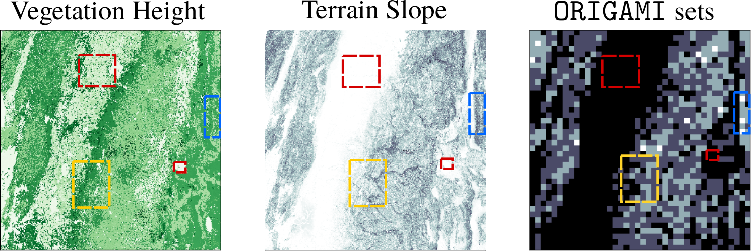
Summary results are provided in Table 5.1. We observe policies based on predictions over ORIGAMI sets to achieve lower decision losses on our test data. Notably, Location predict fails to correctly predict any wildfire location during testing, suggesting generalization at the fine-grained scale with the amount of data available is not possible. Predicting ORIGAMI set membership ( and sets) reaches a considerably higher accuracy. Fig.5.1 provides an example of the sets produced by ORIGAMI: the regions (in shades of grey) are indicative of features the decision loss is based on.
| Pipeline | Predict acc. | Decision loss |
|---|---|---|
| Random action | N/A | |
| Direct policy | N/A | |
| Location predict | ||
| ORIGAMI (5) | ||
| ORIGAMI (10) |
5.2 Active Learning
We apply ORIGAMI to large neural network supervised training with limited data. In particular, we use the average H-entropy of sets generated by folding the simplex of classes as guidance to acquire additional data. The active learning setting typically involves two interleaved stages: a training stage, where the network is optimized given available data, and an acquisition stage, where a new batch is acquired44 4 See (Wang et al. 2016) for other acquisition strategies in deep active learning..
Experimental details
In each run, we optimize an ensemble of ViT (Dosovitskiy et al. 2020) models for image classification on the standard CIFAR100 dataset. We start with a single batch of images, and each epoch we extend the dataset with an additional batch of images constructed following a particular procedure. We compare three different acquisition strategies: (1) random, in which we sample a new batch of images uniformly from all classes, (2) worst- class, which constructs a new sample of images from the classes with lowest marginal accuracy (3) ORIGAMI, where we sample uniformly from the top set in the partition generated by ORIGAMI, ranked by highest average H-entropy. To build ORIGAMI sets, we use a decision loss where each model is an action, such that , , and each entry in is the average loss of each model on all instances of a given class.
Results
We provide results in Table 5.2. With epochs and training and a total dataset of k images, we reach % accuracy when ORIGAMI is used as the acquisition method. We observe a quick drop off when inspecting test performance on the worst classes ordered by marginal accuracy, with ORIGAMI having an overall higher worst-case accuracy. Sampling according to highest H-entropy ensures marginal accuracy across classes is balanced, with new data acquired for classes on which the ensemble is struggling.
| Acquisition | All classes | bot- | bot- |
|---|---|---|---|
| Random | % | % | % |
| Worst- | % | % | % |
| Worst- | % | % | % |
| ORIGAMI | % | % | % |
5.3 Amortized ORIGAMI
The vertex objective introduced in §4.3 considerably improves the computation cost of obtaining good abstractions by means of iterative folding when compared to the other methods discussed. An alternative solution is to instead amortize the cost of computing the Bayes optimal objective (3) by pre-training a neural network approximator to match it on a dataset of loss matrices. In the following, we discuss preliminary results and observations, emerging from training a simple neural network to fit the map on synthetic loss matrices .
With the space of all upper triangular matrices (), we define the neural network with parameters .
We perform training by providing supervision to the model in the form of tuples , where the are produced offline by the Monte Carlo approximation of the integral objective feeding with .
The neural network parameters are then optimized via standard gradient methods to minimize a relative mean-square error objective between the model’s predictions and target Bayes optimal folding costs. Such a model can be then invoked during iterative folding as a surrogate for other variants. Time and compute resources to build a dataset and train the model are thus traded for speedups at inference time when fast evaluation of the folding algorithm is prioritized.
Experimental Details
We test the amortized procedure on a dataset of uniformly sampled loss matrices . The number of actions is fixed to 2 while ranges from (the minimum significant number of classes) to . This choice is due to the fact that all algorithms scale linearly with the number of actions and we are mainly interested in amortizing the quadratic scaling with . The ground-truth integral folding objectives in the form of the upper triangular matrices have then computed with the Monte Carlo procedure detailed in §4.1 using particles. The neural network comprises four layers with 64 neurons each. The loss matrices are flattened and passed to which returns vectors of dimension , corresponding to the predicted non-zero entries of .
Results
The model, trained for 500 epochs for all values of is evaluated via a test set of additional tuples in terms of RMSE loss and accuracy in predicting the optimal folding indices. We observe that the prediction accuracy rapidly decreases with the number of classes while the test RMSE loss increases, as reported by Fig. 5.2. This indicates that the learning problem becomes increasingly difficult with and the folding cannot be amortized by a simple neural architecture. Nonetheless, in the region where the amortized model is accurate, i.e. for , we report a significant speedup (several orders of magnitude) compared to equipped with integral and vertex objectives.
6 Related Work
Multiple studies have taken a utility-theoretic perspective on learning and inference. The utility structure of problems has been leveraged in procedures for formulating abstractions of classes and actions as disjunctions (Horvitz and Klein 1993). A decision-making perspective has also been used to guide abstraction for simplifying probabilistic inference (Poh et al. 1994). Work includes efforts to drive the heterogeneous costs of misclassification into the objective functions and machine learning training procedures (Bach et al. 2006b). Recent work has explored the end-to-end consideration of the quality of decisions in combinatorial optimization (Wilder et al. 2019) and in human-AI collaboration (Wilder et al. 2020). Dubois et al. 2021 propose to leverage knowledge of downstream tasks for compression, improving compression rates over task-agnostic methods. Zhao et al. 2021 formalize a new family of divergences, where discrepancy between distributions is measured through the optimal decision loss induced by each. H-entropy has seen use in Bayesian optimization (Neiswanger et al. 2022), where a new family of acquisition functions is developed.
7 Discussion
We identify and outline several extensions related to the introduction of algorithms in other deep learning domains, dynamic decision-making problems and numerical simulation.
Dynamic ORIGAMI
We have so far discussed static abstractions synthesized by as a fixed set of sets of outcomes. However, as decision losses can change in time e.g., if decision matrix has an explicit dependence on time, the abstractions should track these new preferences. This can take place by applying a modified algorithm able to unfold and fold, instead of starting anew each time.
Folding for simulation
The process of quantization and creation of abstractions via ORIGAMI can be loosely connected to meshing and discretization techniques ubiquitous in graphics and numerical simulation of differential equations (Plewa et al. 2005). Instead of standard metrics to guide discretization, is driven by utilities and is not constrained to sets that are local in space or time. As shown in our experiments, geographical regions found via can involve disjoint subregions. Locality can be enforced or promoted via minimal changes to the method.
Adaptive tokenization
The folding problem formalized by ORIGAMI is closely related to tokenization procedures common in natural language processing and computer vision. It may be fruitful to investigate adaptive tokenization strategies using the machinery developed in this work, using other surrogates or estimators for the decision loss .
8 Conclusion
We presented methods that guide the formulation of abstractions to simplify learning problems based on a careful consideration of downstream decisions. The distillation of abstractions enables data-efficient learning of predictive models. We derive a class of iterative algorithms we refer to as ORIGAMI that work to reduce the dimensionality of the probability simplex while preserving information useful for downstream decisions. In doing so, the method progressively hides information that is not necessary to implement optimal policies, allowing predictive models to learn over sets rather than fine-grained outcomes without loss in decision quality.
References
- Azuma et al. (2006) R. Azuma, M. Daily, and C. Furmanski. A review of time critical decision making models and human cognitive processes. In 2006 IEEE aerospace conference, pages 9–pp. IEEE, 2006.
- Bach et al. (2006a) F. R. Bach, D. Heckerman, and E. Horvitz. Considering cost asymmetry in learning classifiers. The Journal of Machine Learning Research, 7:1713–1741, 2006a.
- Bach et al. (2006b) F. R. Bach, D. Heckerman, and E. Horvitz. Considering cost asymmetry in learning classifiers. The Journal of Machine Learning Research, 7:1713–1741, 2006b.
- Bommasani et al. (2021) R. Bommasani, D. A. Hudson, E. Adeli, R. Altman, S. Arora, S. von Arx, M. S. Bernstein, J. Bohg, A. Bosselut, E. Brunskill, et al. On the opportunities and risks of foundation models. arXiv preprint arXiv:2108.07258, 2021.
- DeGroot (1962) M. H. DeGroot. Uncertainty, information, and sequential experiments. The Annals of Mathematical Statistics, 33(2):404–419, 1962.
- Dosovitskiy et al. (2020) A. Dosovitskiy, L. Beyer, A. Kolesnikov, D. Weissenborn, X. Zhai, T. Unterthiner, M. Dehghani, M. Minderer, G. Heigold, S. Gelly, et al. An image is worth 16x16 words: Transformers for image recognition at scale. arXiv preprint arXiv:2010.11929, 2020.
- Dubois et al. (2021) Y. Dubois, B. Bloem-Reddy, K. Ullrich, and C. J. Maddison. Lossy compression for lossless prediction. Advances in Neural Information Processing Systems, 34:14014–14028, 2021.
- Group (1996) N. W. C. Group. Wildland fire suppression tactics reference guide, 1996.
- Hartman (1959) P. Hartman. On functions representable as a difference of convex functions. Pacific Journal of Mathematics, 9(3):707–713, 1959.
- Hersbach et al. (2020) H. Hersbach, B. Bell, P. Berrisford, S. Hirahara, A. Horányi, J. Muñoz-Sabater, J. Nicolas, C. Peubey, R. Radu, D. Schepers, et al. The era5 global reanalysis. Quarterly Journal of the Royal Meteorological Society, 146(730):1999–2049, 2020.
- Ho (2019) M. K. Ho. The value of abstraction. Current opinion in behavioral sciences, 29, 2019.
- Horvitz and Klein (1993) E. Horvitz and A. C. Klein. Utility-based abstraction and categorization. In Proceedings of Uncertainty in Artificial Intelligence, pages 128–135, 1993.
- Horvitz and Barry (1995) E. J. Horvitz and M. Barry. Display of information for time-critical decision making. In Proceedings of Uncertainty in Artificial Intelligence, pages 296––305, 1995.
- Jain et al. (2020) P. Jain, S. C. Coogan, S. G. Subramanian, M. Crowley, S. Taylor, and M. D. Flannigan. A review of machine learning applications in wildfire science and management. Environmental Reviews, 28(4):478–505, 2020.
- Kapoor and Horvitz (2009) A. Kapoor and E. Horvitz. Breaking boundaries: Active information acquisition across learning and diagnosis. Advances in neural information processing systems, 2009.
- Lindig-León et al. (2019) C. Lindig-León, S. Gottwald, and D. A. Braun. Analyzing abstraction and hierarchical decision-making in absolute identification by information-theoretic bounded rationality. Frontiers in neuroscience, 13:1230, 2019.
- Lipp and Boyd (2016) T. Lipp and S. Boyd. Variations and extension of the convex–concave procedure. Optimization and Engineering, 17(2):263–287, 2016.
- Litjens et al. (2022) G. Litjens, F. Ciompi, and J. van der Laak. A decade of gigascience: The challenges of gigapixel pathology images. GigaScience, 11, 2022.
- Loshchilov and Hutter (2017) I. Loshchilov and F. Hutter. Decoupled weight decay regularization. arXiv preprint arXiv:1711.05101, 2017.
- Neiswanger et al. (2022) W. Neiswanger, L. Yu, S. Zhao, C. Meng, and S. Ermon. Generalizing bayesian optimization with decision-theoretic entropies. arXiv preprint arXiv:2210.01383, 2022.
- Plewa et al. (2005) T. Plewa, T. Linde, V. G. Weirs, et al. Adaptive mesh refinement-theory and applications. 2005.
- Poh et al. (1994) K. L. Poh, M. Fehling, and E. Horvitz. Dynamic construction and refinement of utility-based categorization models. IEEE Transactions on Systems, Man, and Cybernetics, 24(11):1653–1663, 1994.
- Rollins (2009) M. G. Rollins. Landfire: a nationally consistent vegetation, wildland fire, and fuel assessment. International Journal of Wildland Fire, 18(3):235–249, 2009.
- Wang et al. (2016) K. Wang, D. Zhang, Y. Li, R. Zhang, and L. Lin. Cost-effective active learning for deep image classification. IEEE Transactions on Circuits and Systems for Video Technology, 27(12):2591–2600, 2016.
- Wightman (2019) R. Wightman. Pytorch image models. https://github.com/rwightman/pytorch-image-models, 2019.
- Wilder et al. (2019) B. Wilder, B. N. Dilkina, and M. Tambe. Melding the data-decisions pipeline: Decision-focused learning for combinatorial optimization. In AAAI, 2019.
- Wilder et al. (2020) B. Wilder, E. Horvitz, and E. Kamar. Learning to complement humans. arXiv preprint arXiv:2005.00582, 2020.
- Zhao et al. (2021) S. Zhao, A. Sinha, Y. He, A. Perreault, J. Song, and S. Ermon. Comparing distributions by measuring differences that affect decision making. In International Conference on Learning Representations, 2021.
- Zheng et al. (2020) D. Zheng, C. Ma, M. Wang, J. Zhou, Q. Su, X. Song, Q. Gan, Z. Zhang, and G. Karypis. Distdgl: distributed graph neural network training for billion-scale graphs. In 2020 IEEE/ACM 10th Workshop on Irregular Applications: Architectures and Algorithms (IA3), pages 36–44. IEEE, 2020.
- Zhou et al. (2019) Z. Zhou, M. M. R. Siddiquee, N. Tajbakhsh, and J. Liang. Unet++: Redesigning skip connections to exploit multiscale features in image segmentation. IEEE transactions on medical imaging, 39(6):1856–1867, 2019.
Ideal Abstractions for Decision-Focused Learning
Supplementary Material
Appendix A Derivations
Proposition 4 (Folding increases H-entropy).
Let and be any sequence of folds. Then,
Proof.
We show the result for each row of and a single fold:
∎
Proposition 5 (H–entropy is minimized on vertices).
The minimizer
is a vertex of
Proof.
Let be the set of vertices of the simplex, i.e. the canonical basis of . We need to show that . Due to convexity of the simplex , the minimizer can be expresses as a convex combination of the vertices, i.e.
By Jensen’s inequality we have
and
so the minimum of over is bounded below by the minimum over the vertices. Since the vertices belong to , the result is proved. ∎
Appendix B Experiments
B.1 Folding for Decision Problems
Dataset curation
We design and build a new dataset named FIRE! that contains active fire information from Visible Infrared Imaging Radiometer Suite (VIIRS) on a spatial resolution of meters, as well as climate and vegetation data.
Fires: We consider fire instances collected over the years and . Each instance contains fire radiative power, location (latitude and longitude) and auxiliary information such as time of day and confidence for the measurement. We select the region spanned by latitude and longitude .
Vegetation: We collect data from the LANDFIRE program. In particular, we add the following features: existing vegetation height (EVH), existing vegetation cover (EVC), existing vegetation type (EVT), slope degrees (SlpD), slope percent rise (slpP), roads, aspect (Asp). As these databases are updates at lower frequencies than VIIRs and climate, we have access to and snapshots which we use as additional context for the model. The region is aligned with VIIRS spatial coordinates.
Climate: We extract a set of climate and weather features from the large-scale ERA5 dataset. Weather and climate variables describe a larger region than latitude and longitude to provide context for the predictive model. All data slices are aligned in time.
Predictive task
The model takes as input a snapshot ( week, aggregated as described above) and is tasked with predicting the location of the largest wildfire (measured in radiative power) in the following week. When using ORIGAMI, spatial locations are clustered according to the decision loss, and thus the dimension of is smaller than the dimension of . We optimize the parameters of all models using a standard binary cross entropy loss.
Decision making and decision loss
We design a simple, deterministic closed-loop policy reliant on predictions made by a deep learning model. Our goal is to investigate whether the quality of a decision policy can be improved by performing upstream prediction on a "simplified" space of locations found as a decision–optimal clustering with ORIGAMI.
Wildfire management actions are: (1) land intervention, (2) aircraft intervention (3) indirect containment, according to the location predicted by the wildfire location model. The decision loss is crafted according to insights extracted from (Group 1996). The following factors are used: fire radiative power, existing vegetation height, roads, temperature, magnitude of wind. In particular, action (1) incurs in high cost when slope and terrain height are larger, (2) when wind is strong, and (3) when vegetation is dense. Since all features are on different scales, we normalized the decision loss to obtain values in a comparable range. We note that the decision loss is not meant to encode all factors one may want to consider for wildfire management, as the experiment is meant to showcase potential applications of ORIGAMI.
Training details
We train the wildfire location predictive model for epochs using the AdamW optimizer (Loshchilov and Hutter 2017), with a learning rate of and a cosine decay schedule to . We set the batch size to (each element of the batch contains a temporal slice of context data, with the model asked to predict the location of the largest wildfire in the following week). All models are standard with layers.
When evaluating the policy, we pick the Bayes optimal wildfire strategy between: (1) land intervention, (2) aircraft intervention (3) indirect containment, according to the location predicted by the wildfire location model.
B.2 Active Learning
Training details
We train ensembles of vision transformers ViT (Dosovitskiy et al. 2020) on the CIFAR100 dataset, starting from a single random batch of data. Each epoch, we increase dataset size by sampling a new batch based on different acquisition methods:
- •
random: a new batch of images is obtained by sampling uniformly from all classes
- •
worst-: the new batch is obtained by sampling data uniformly if the corresponding label belongs to the classes with lowest marginal accuracy
- •
ORIGAMI: we apply ORIGAMI to generate a partition of all classes. We select the set of classes in the partition with highest average H-entropy, and sample uniformly.
We use ViT-base from the timm library (Wightman 2019) with patch size and latent dimension , and add the logits of each model in the ensemble before computing the cross-entropy loss. We train all models epochs using AdamW optimizer (Loshchilov and Hutter 2017), a learning rate schedule with epochs of linear warmup ( to ) followed by cosine decay down to . We use batch size .