跳到论文正文
W Papers独立论文阅读器 arXiv:2303.17052 论文正文 计算阅读时间 · 0%
引用这篇论文根据当前论文元数据生成,正式投稿前建议核对。


License: CC BY 4.0
arXiv:2303.17052v1 [nlin.SI] 29 Mar 2023

Rogue waves arising on the standing periodic waves
in the Ablowitz-Ladik equation

Jinbing Chen J. ChenSchool of Mathematics, Southeast University, Nanjing, Jiangsu 210096, P.R. China Email address: cjb@seu.edu.cn and Dmitry E. Pelinovsky D.E. Pelinovsky, Corresponding author Department of Mathematics, McMaster University, Hamilton, Ontario, Canada, L8S 4K1 Email address: dmpeli@math.mcmaster.ca
Date: August 11, 2026
Abstract.

We study the standing periodic waves in the semi-discrete integrable system modelled by the Ablowitz–Ladik equation. We have related the stability spectrum to the Lax spectrum by separating the variables and by finding the characteristic polynomial for the standing periodic waves. We have also obtained rogue waves on the background of the modulationally unstable standing periodic waves by using the end points of spectral bands and the corresponding eigenfunctions. The magnification factors for the rogue waves have been computed analytically and compared with their continuous counterparts. The main novelty of this work is that we explore a non-standard linear Lax system, which is different from the standard Lax representation of the Ablowitz–Ladik equation.

Key words and phrases: 
Ablowitz-Ladik equation, standing periodic waves, Lax spectrum, stability spectrum, rogue waves

This article is dedicated to Athanassios S. Fokas on the occasion of his 70th anniversary for his many contributions to studies of integrable nonlinear PDEs and boundary-value problems.

1. Introduction

The nonlinear Schrödinger (NLS) equation models wave dynamics in many physical problems related to fluids, plasmas, and optics [21, 32]. Complicated wave patterns can be expressed analytically by using exact solutions of the NLS equation for periodic and double-periodic standing waves (see review in [30]). The standing periodic waves are known to be modulationally unstable [17, 18] and rogue waves (localized perturbations in space and time) have been observed on their backgrounds in numerical experiments [3, 27]. Rogue waves are generated due to modulational instability of the wave background [16, 19]. The exact solutions for rogue waves arising on the periodic stading waves were obtained analytically [8, 13, 20] and confirmed experimentally for fluids and optics [36].

It is natural to ask if the modulational instability and rogue waves persist on the standing periodic waves in the integrable discretizations of the integrable NLS equation. This question has received much less attention in the literature. The main purpose of our work is to answer this question for the Ablowitz-Ladik (AL) equation [1] written in the normalized form:

i​u˙n+(1+|un|2)​(un+1+un−1)=0,i\dot{u}_{n}+(1+|u_{n}|^{2})(u_{n+1}+u_{n-1})=0, (1.1)

where the dot represents the derivative of {un​(t)}n∈ℤ∈ℂℤ\{u_{n}(t)\}_{n\in\mathbb{Z}}\in\mathbb{C}^{\mathbb{Z}} with respect to the time variable t∈ℝt\in\mathbb{R}, and i=−1i=\sqrt{-1}. The continuum limit of the AL equation (1.1) is obtained for slowly varying wave packets of small amplitude, the leading order of which can be represented as

un​(t)=ε​𝔲​(ε​n,ε2​t)​e2​i​t,u_{n}(t)=\varepsilon\mathfrak{u}(\varepsilon n,\varepsilon^{2}t)e^{2it}, (1.2)

where ε>0\varepsilon>0 is a formal small parameter. Substituting (1.2) into (1.1) and expanding 𝔲⁡(X±ε,T)\mathfrak{u}(X\pm\varepsilon,T) with X=ε​nX=\varepsilon n and T=ε2​tT=\varepsilon^{2}t in the Taylor series in ε\varepsilon yield at the formal order of 𝒪⁡(ε3)\mathcal{O}(\varepsilon^{3}) the continuous NLS equation in the form:

i​𝔲T+𝔲X​X+2​|𝔲|2​𝔲=0.i\mathfrak{u}_{T}+\mathfrak{u}_{XX}+2|\mathfrak{u}|^{2}\mathfrak{u}=0. (1.3)

Rogue waves on the constant-amplitude wave background have been obtained for the AL equation (1.1) and related discrete equations in [4, 5, 29, 38]. They have been observed in numerical experiments [2]. Higher-order rogue waves have been studied by using the inverse scattering method [14]. Further generalization of these rogue waves to fully discrete integrable NLS equation was recently given in [28]. What we will develop in this work is the construction of rogue waves on the background of discrete standing periodic waves. The discrete periodic and double-periodic waves were obtained previously for the AL equation in [15, 23, 24].

In a series of recent works, we have constructed rogue waves on the background of standing periodic waves in the continuous integrable models including the NLS equation [8, 13], the derivative NLS equation [10, 12], the modified KdV equation [7, 9], and the sine–Gordon equation [31]. The latest work in this series was the first construction of such rogue waves in the discrete modified KdV equation [11]. In all works, we used the nonlinearization method [6, 34] which allowed us to characterize the standing periodic waves as the restriction of solutions of nonlinear models as squared solutions of the linear Lax equations.

However, we have failed to characterize the discrete standing periodic waves by using constraints of the nonlinearization method for the AL equation (developed in [22, 35]) because the constraints generate difference equations which are not satisfied by the standing periodic waves. As a result, we had to develop new ideas based on separation of variables for the standing periodic waves in the linear Lax equations. This separation of variables is similar to the approach in [17] used to characterize the modulational stability of standing periodic waves in the continuous NLS equation. With this approach, we can obtain analytically the end points of spectral bands of the Lax spectrum and the corresponding eigenfunctions, which are then used to obtain the rogue wave solutions on the background of discrete standing periodic waves.

Integrability of the AL equation can be expressed by using two different Lax formulations. The standard formulation explored previously in the context of rogue waves on the constant-amplitude wave background [4, 14, 29] is irrelevant for the modulational stability and rogue waves on the standing periodic waves due to several issues: (i) the location of the Lax spectrum is different, (ii) there exists no relation between squared eigenfunctions and the linearized AL equation, and consequently, (iii) the rogue waves are not properly defined. On the other hand, we show here that the alternative formulation related to symplectic integrable map of the nonlinearization method in [22] allows us to fix issues (i), (ii), and (iii) and to describe properties of the rogue waves on the standing periodic wave background. The main novelty of our work is that our results are derived from non-standard Lax formulation of the AL equation.

Among possible applications of our main results, we can mention recent studies of breathers and rogue waves in non-integrable discrete settings [33]. Many numerical results are based on the homotopy continuation of breathers and rogue waves from their integrable limits expressed by the AL equation. With the precise construction of the standing periodic waves and their rogue waves, we can then utilize these solutions in the homotopy continuation towards the nonintegrable versions of the discrete NLS equations.

The article is organized as follows. Section 2 presents the main results of our computations. Section 3 establishes the relation between squared eigenfunctions of the linear Lax equations and solutions of the linearized AL equation. Section 4 presents analytical and numerical approximations of the Lax and stability spectra. Section 5 gives construction of nonperiodic solutions of the linear Lax equations in terms of periodic eigenfunctions. Section 6 explains how the Darboux transformation is used to obtain the rogue wave solutions from the nonperiodic solutions of the linear Lax equations and to study magnification factors of the rogue waves.

2. Lax pair, standing periodic waves, and rogue waves

The AL equation (1.1) can be represented as the compatibility condition for a Lax pair of linear equations:

φn+1=U⁡(un,λ)​φn,φ˙n=V⁡(un,λ)​φn,\varphi_{n+1}=U(u_{n},\lambda)\varphi_{n},\qquad\dot{\varphi}_{n}=V(u_{n},\lambda)\varphi_{n}, (2.1)

defined by the matrices

U⁡(un,λ)=11+|un|2​(λun−u¯nλ−1)\displaystyle U(u_{n},\lambda)=\frac{1}{\sqrt{1+|u_{n}|^{2}}}\left(\begin{array}[]{cc}\lambda&u_{n}\\ -\bar{u}_{n}&\lambda^{-1}\\ \end{array}\right)

and

V⁡(un,λ)=i⁡(12​(λ2+λ−2+un​u¯n−1+u¯n​un−1)λ​un−λ−1​un−1−λ​u¯n−1+λ−1​u¯n−12​(λ2+λ−2+un​u¯n−1+u¯n​un−1)),\displaystyle\qquad V(u_{n},\lambda)=i\left(\begin{array}[]{cc}\frac{1}{2}\left(\lambda^{2}+\lambda^{-2}+u_{n}\bar{u}_{n-1}+\bar{u}_{n}u_{n-1}\right)&\lambda u_{n}-\lambda^{-1}u_{n-1}\\ -\lambda\bar{u}_{n-1}+\lambda^{-1}\bar{u}_{n}&-\frac{1}{2}\left(\lambda^{2}+\lambda^{-2}+u_{n}\bar{u}_{n-1}+\bar{u}_{n}u_{n-1}\right)\\ \end{array}\right),

where {φn}n∈ℤ∈(ℂ2)ℤ\{\varphi_{n}\}_{n\in\mathbb{Z}}\in(\mathbb{C}^{2})^{\mathbb{Z}} depends on time tt, λ∈ℂ\lambda\in\mathbb{C} is a spectral parameter which is constant in nn and tt, and u¯n​(t)\bar{u}_{n}(t) denotes the complex-conjugate of un​(t)u_{n}(t).

Remark 1.

There exists a simpler Lax pair,

φn+1=U⁡(un,λ)​φn,U⁡(un,λ)=(λun−u¯nλ−1),\varphi_{n+1}=U(u_{n},\lambda)\varphi_{n},\quad U(u_{n},\lambda)=\left(\begin{array}[]{cc}\lambda&u_{n}\\ -\bar{u}_{n}&\lambda^{-1}\\ \end{array}\right), (2.2)

and

φ˙n=V⁡(un,λ)​φn,V⁡(un,λ)=i⁡(12​(λ2+λ−2)+un​u¯n−1λ​un−λ−1​un−1−λ​u¯n−1+λ−1​u¯n−12​(λ2+λ−2)−u¯n​un−1),\dot{\varphi}_{n}=V(u_{n},\lambda)\varphi_{n},\ V(u_{n},\lambda)=i\left(\begin{array}[]{cc}\frac{1}{2}\left(\lambda^{2}+\lambda^{-2}\right)+u_{n}\bar{u}_{n-1}&\lambda u_{n}-\lambda^{-1}u_{n-1}\\ -\lambda\bar{u}_{n-1}+\lambda^{-1}\bar{u}_{n}&-\frac{1}{2}\left(\lambda^{2}+\lambda^{-2}\right)-\bar{u}_{n}u_{n-1}\\ \end{array}\right), (2.3)

commutativity of which also yields the AL equation (1.1). We have found that the stability spectrum of the standing periodic waves can be characterized from the Lax spectrum associated with the linear system (2.1) due to the squared eigenfunction relation, however, we did not find the squared eigenfunction relation for eigenfunctions of the linear system (2.2)–(2.3).

We consider the standing wave solution of the AL equation (1.1) in the form:

un​(t)=Un​e2​i​ω​t,u_{n}(t)=U_{n}e^{2i\omega t}, (2.4)

where {Un}n∈ℤ∈ℂℤ\{U_{n}\}_{n\in\mathbb{Z}}\in\mathbb{C}^{\mathbb{Z}} and ω∈ℝ\omega\in\mathbb{R} is a frequency parameter. The AL equation (1.1) with the standing wave reduction (2.4) becomes the second-order difference equation

(1+|Un|2)​(Un+1+Un−1)=2​ω​Un,n∈ℤ.(1+|U_{n}|^{2})(U_{n+1}+U_{n-1})=2\omega U_{n},\quad n\in\mathbb{Z}. (2.5)

It can be integrated with two conserved quantities as in the following lemma.

Lemma 1.

Let {Un}n∈ℤ∈ℂℤ\{U_{n}\}_{n\in\mathbb{Z}}\in\mathbb{C}^{\mathbb{Z}} be a solution of the difference equation (2.5). Then, the following real-valued quantities

F0:=i⁡(Un​U¯n−1−U¯n​Un−1)F_{0}:=i(U_{n}\bar{U}_{n-1}-\bar{U}_{n}U_{n-1}) (2.6)

and

F1:=ω⁡(Un​U¯n−1+U¯n​Un−1)−|Un|2−|Un−1|2−|Un|2​|Un−1|2F_{1}:=\omega(U_{n}\bar{U}_{n-1}+\bar{U}_{n}U_{n-1})-|U_{n}|^{2}-|U_{n-1}|^{2}-|U_{n}|^{2}|U_{n-1}|^{2} (2.7)

are constant in n∈ℤn\in\mathbb{Z}.

Proof.

By multiplying (2.5) by U¯n\bar{U}_{n} and subtracting the complex conjugate, we obtain

(1+|Un|2)​[(Un+1​U¯n−U¯n+1​Un)−(Un​U¯n−1−U¯n​Un−1)]=0,(1+|U_{n}|^{2})[(U_{n+1}\bar{U}_{n}-\bar{U}_{n+1}U_{n})-(U_{n}\bar{U}_{n-1}-\bar{U}_{n}U_{n-1})]=0,

from which conservation of F0F_{0} follows.

Similarly, multiplying (2.5) by U¯n−1\bar{U}_{n-1} and by U¯n+1\bar{U}_{n+1} and adding the complex conjugate yield

(1+|Un|2)​|Un+1|2−ω⁡(Un​U¯n+1+U¯n​Un+1)=(1+|Un|2)​|Un−1|2−ω⁡(Un​U¯n−1+U¯n​Un−1),(1+|U_{n}|^{2})|U_{n+1}|^{2}-\omega(U_{n}\bar{U}_{n+1}+\bar{U}_{n}U_{n+1})=(1+|U_{n}|^{2})|U_{n-1}|^{2}-\omega(U_{n}\bar{U}_{n-1}+\bar{U}_{n}U_{n-1}),

from which conservation of F1F_{1} follows. ∎

Periodic waves with trivial phase are given by real-valued periodic solutions of the difference equation (2.5) with F0=0F_{0}=0 in (2.6). Two families were obtained in [11] (see also [23, 24]), which we refer to as the dnoidal and cnoidal waves. The dnoidal waves are given in the form:

Un=sn⁡(α,k)cn⁡(α,k)​dn​(α​n,k),ω=dn⁡(α,k)cn2​(α,k),U_{n}=\frac{{\rm sn}(\alpha;k)}{{\rm cn}(\alpha;k)}{\rm dn}(\alpha n;k),\qquad\omega=\frac{{\rm dn}(\alpha;k)}{{\rm cn}^{2}(\alpha;k)}, (2.8)

with two parameters of α∈(0,K⁡(k))\alpha\in(0,K(k)) and k∈(0,1)k\in(0,1), where kk is the elliptic modulus.

  • •

    As k→0k\to 0, the dnoidal wave degenerates to the constant-amplitude wave

    Un=tan⁡(α),ω=sec2​(α),α∈(0,π2),U_{n}=\tan(\alpha),\qquad\omega={\rm sec}^{2}(\alpha),\qquad\alpha\in\left(0,\frac{\pi}{2}\right), (2.9)
  • •

    As k→1k\to 1, the dnoidal wave degenerates into the solitary wave

    Un=sinh⁡(α)​sech​(α​n),ω=cosh⁡(α),α∈(0,∞).U_{n}=\sinh(\alpha){\rm sech}(\alpha n),\qquad\omega=\cosh(\alpha),\qquad\alpha\in(0,\infty). (2.10)

The cnoidal waves are given in the form:

Un=k​sn​(α,k)dn⁡(α,k)​cn​(α​n,k),ω=cn⁡(α,k)dn2​(α,k),U_{n}=\frac{k{\rm sn}(\alpha;k)}{{\rm dn}(\alpha;k)}{\rm cn}(\alpha n;k),\qquad\omega=\frac{{\rm cn}(\alpha;k)}{{\rm dn}^{2}(\alpha;k)}, (2.11)

with two parameters of α∈(0,2​K​(k))\alpha\in(0,2K(k)) and k∈(0,1)k\in(0,1). The limit k→0k\to 0 gives the trivial solution, whereas the limit k→1k\to 1 gives the same solitary wave (2.10).

The standing waves in the limit α→0\alpha\to 0 recover the asymptotic approximation (1.2) with ε=α\varepsilon=\alpha. Since

sn⁡(α,k)=α+𝒪⁡(α3),cn⁡(α,k)=1−12​α2+𝒪⁡(α4),dn⁡(α,k)=1−12​k2​α2+𝒪⁡(α4),\displaystyle{\rm sn}(\alpha;k)=\alpha+\mathcal{O}(\alpha^{3}),\quad{\rm cn}(\alpha;k)=1-\frac{1}{2}\alpha^{2}+\mathcal{O}(\alpha^{4}),\quad{\rm dn}(\alpha;k)=1-\frac{1}{2}k^{2}\alpha^{2}+\mathcal{O}(\alpha^{4}),

the dnoidal and cnoidal waves of the AL equation (1.1) yield solutions

𝔲⁡(X,T)=ei⁡(2−k2)​T​dn​(X,k),𝔲⁡(X,T)=ei⁡(2​k2−1)​T​k​cn​(X,k),\mathfrak{u}(X,T)=e^{i(2-k^{2})T}{\rm dn}(X;k),\qquad\mathfrak{u}(X,T)=e^{i(2k^{2}-1)T}k{\rm cn}(X;k),

which are the dnoidal and cnoidal waves of the continuous NLS equation (1.3).

Remark 2.

Since the continuous NLS equation (1.3) also has a family of the standing periodic waves with nontrivial phase [13, 17], we conjecture that there exist complex-valued periodic solutions of the difference equation (2.5) with F0≠0F_{0}\neq 0 in (2.6). However, such solutions are not considered in our work.

Figures 1 and 2 present the main results which are the rogue waves on the dnoidal and cnoidal wave backgrounds. We have obtained the rogue waves by using only analytical methods with the following steps:

  • (i)

    characterizing end points of the spectral bands associated with standing periodic waves,

  • (ii)

    computing the corresponding periodic eigenfunctions for the end-point eigenvalues,

  • (iii)

    representing the second solutions of the linear system for the end-point eigenvalues,

  • (iv)

    performing the 1-fold Darboux transformation (DT) on the standing periodic waves with the periodic and nonperiodic eigenfunctions in (ii) and (iii).

Numerical approximations are only used to represent the rogue waves graphically.

Refer to caption
Refer to caption
Refer to caption
Refer to caption
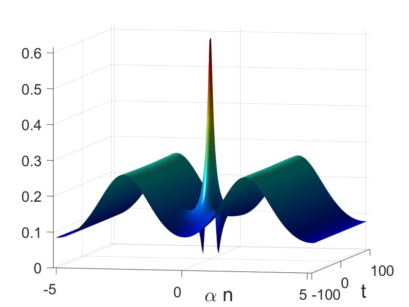
Figure 1. New solutions on the background of the dnoidal wave (2.8). Left: profiles of unu_{n} and vn:=u^nv_{n}:=\hat{u}_{n} versus α​n\alpha n obtained from the 1-fold DT with the periodic eigenfunctions. Right: solution surface |u^n​(t)||\hat{u}_{n}(t)| versus α​n\alpha n and tt obtained from the 1-fold DT with the nonperiodic eigenfunctions. Top and bottom panels show rogue waves for two different end-point eigenvalues of the Lax spectrum.

Figure 1 shows the new solutions obtained by using the 1-fold DT on the background of the dnoidal wave (2.8). The top panels correspond to the choice of λ=λ1\lambda=\lambda_{1} and the bottom panels correspond to the choice of λ=λ2\lambda=\lambda_{2}, see (4.6) and (4.7) below. The left panels show the profiles of unu_{n} and vnv_{n} versus α​n\alpha n, where unu_{n} is the dnoidal wave (2.8) and vnv_{n} is a new solution obtained with the periodic eigenfunctions after the 1-fold DT. The new solution is a half-period translation of the original dnoidal wave with the sign flip for λ=λ2\lambda=\lambda_{2} and with no sign flip for λ=λ1\lambda=\lambda_{1}. The right panels show the solution surface of |u^n​(t)||\hat{u}_{n}(t)| versus α​n\alpha n and tt, where u^n\hat{u}_{n} is a new solution obtained with the nonperiodic eigenfunctions after the 1-fold DT. The new solution is an isolated rogue wave on the background of the half-period translated dnoidal wave.

As a practical outcome of the exact solutions, we can compute the magnification factor of the rogue waves as the quotient between the maximal amplitude of the rogue wave and the maximal amplitude of the dnoidal wave background. We have seen from Figure 1 that the maximal amplitude of the rogue wave is attained at n=0n=0 and t=0t=0, where we have computed analytically the magnification factor in the closed form:

Mdn​(α,k)=1+1−σ1​1−k2dn⁡(α,k),M_{\rm dn}(\alpha,k)=1+\frac{1-\sigma_{1}\sqrt{1-k^{2}}}{{\rm dn}(\alpha;k)}, (2.12)

with σ1=−1\sigma_{1}=-1 for λ=λ1\lambda=\lambda_{1} and σ1=+1\sigma_{1}=+1 for λ=λ2\lambda=\lambda_{2}. In the continuum limit α→0\alpha\to 0, it converges to Mdn​(α,k)→2−σ1​1−k2M_{\rm dn}(\alpha,k)\to 2-\sigma_{1}\sqrt{1-k^{2}}, which reproduces the correct expression for the magnification factor of the dnoidal wave in the continuous NLS equation (1.3) obtained in [8].

The rogue wave associated with λ1\lambda_{1} has a bigger magnification factor than the one associated with λ2\lambda_{2}. Since eigenvalues satisfy the order

0<λ1<λ2<1<λ2−1<λ1−1,0<\lambda_{1}<\lambda_{2}<1<\lambda_{2}^{-1}<\lambda_{1}^{-1},

we associate this difference with the fact that λ1\lambda_{1} is located further from the unit circle compared to λ2\lambda_{2} in the Lax spectrum of the dnoidal wave, see Figure 3 below. The same rogue waves are computed from reflected eigenvalues λ1−1\lambda_{1}^{-1} and λ2−1\lambda_{2}^{-1} and from negative eigenvalues −λ1-\lambda_{1}, −λ2-\lambda_{2}, −λ1−1-\lambda_{1}^{-1}, and −λ2−1-\lambda_{2}^{-1}, which exist due to the symmetry of the Lax system (2.1).

Refer to caption
Refer to caption
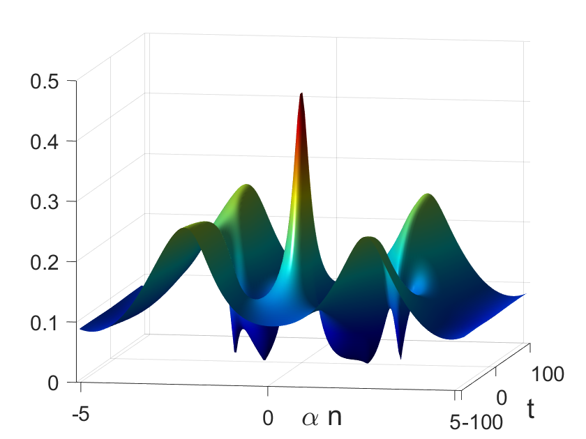
Figure 2. The same as on Figure 1 but for the cnoidal wave (2.11) for one end-point eigenvalue of the Lax spectrum.

Figure 2 shows the new solutions obtained by using the 1-fold DT on the background of the cnoidal wave (2.11). The profiles of |un||u_{n}| and |vn||v_{n}| versus α​n\alpha n on a single period are shown on the left panel, where vnv_{n} is a new solution obtained with the periodic eigenfunctions after the 1-fold DT. The new solution is a quarter-period translation of the original cnoidal wave with a phase factor. The solution surface of |u^n​(t)||\hat{u}_{n}(t)| versus α​n\alpha n and tt is shown on the right panel, where u^n\hat{u}_{n} is a new solution obtained with the nonperiodic eigenfunctions after the 1-fold DT. The new solution is an isolated rogue wave on the background of the quarter-period translated cnoidal wave. Rogue waves associated with the reflected eigenvalues due to complex conjugation, reflection about the unit circle, and the sign reflection are displayed by similar solution surfaces since the complex phase is neglected in plotting of |u^n​(t)||\hat{u}_{n}(t)|.

We have observed from Figure 2 that the maximal value of |u^n​(t)||\hat{u}_{n}(t)| is not attained at n=0n=0 and t=0t=0. However, it is attained at a point located very close to the origin, therefore, a good approximation of the magnification factor can still be computed at n=0n=0 and t=0t=0, where we have computed analytically the magnification factor for the rogue wave in the closed form:

Mcn​(α,k)=1+1dn⁡(α,k).\displaystyle M_{\rm cn}(\alpha,k)=1+\frac{1}{{\rm dn}(\alpha;k)}. (2.13)

In the continuum limit α→0\alpha\to 0, it converges to Mcn​(α,k)→2M_{\rm cn}(\alpha,k)\to 2, which reproduces the double magnification factor of the cnoidal wave in the continuous NLS equation (1.3) obtained in [8].

Note that the magnification factors of the dnoidal and cnoidal waves for the continuous NLS equation (1.3) have been verified experimentally in [36]. These main results suggest new experiments in the discrete setting modeled by the AL equation (1.1) and other nonintegrable discretizations of the NLS equation (1.3).

Among other main results of this work, we mention the squared eigenfunction relation between solutions of the linearized AL equation and the linear Lax equations, see Lemma 2 below. This allows us to connect the Lax spectrum and the stability spectrum and to characterize the periodic eigenfunctions of the linear Lax system from the standing periodic waves, see Corollary 1, Corollary 2, and Lemma 3.15 below. The Lax spectrum and the stability spectrum for the constant-amplitude wave are obtained analytically, see Lemma 4 below. However, we have to approximate the Lax spectrum numerically for the dnoidal and cnoidal waves. It follows from these numerical approximations that both the dnoidal and cnoidal waves are modulationally unstable. Finally, we give analytical expressions for the nonperiodic eigenfunctions in Lemma 5 and 6 below and we present the 1-fold DT in the closed form in Lemma 7 below.

3. Spectral stability of standing periodic waves

Here we will set up the spectral stability problem for the standing periodic waves and relate its eigenfunctions with squared eigenfunctions of the linear system (2.1).

The spectral stability of the standing waves of the form (2.4) in the time evolution of the AL equation (1.1) can be studied by adding a perturbation of the form

un​(t)=e2​i​ω​t​[Un+vn​(t)].u_{n}(t)=e^{2i\omega t}[U_{n}+v_{n}(t)]. (3.1)

Substituting (3.1) into the AL equation (1.1) and truncating at the linear terms in vnv_{n} gives rise to the linearized AL equation

i​v˙n−2​ω​vn+(1+|Un|2)​(vn+1+vn−1)+(Un+1+Un−1)​(Un​v¯n+U¯n​vn)=0i\dot{v}_{n}-2\omega v_{n}+(1+|U_{n}|^{2})(v_{n+1}+v_{n-1})+(U_{n+1}+U_{n-1})(U_{n}\bar{v}_{n}+\bar{U}_{n}v_{n})=0 (3.2)

and its complex conjugate equation

−i​v¯˙n−2​ω​v¯n+(1+|Un|2)​(v¯n+1+v¯n−1)+(U¯n+1+U¯n−1)​(U¯n​vn+Un​v¯n)=0.-i\dot{\bar{v}}_{n}-2\omega\bar{v}_{n}+(1+|U_{n}|^{2})(\bar{v}_{n+1}+\bar{v}_{n-1})+(\bar{U}_{n+1}+\bar{U}_{n-1})(\bar{U}_{n}v_{n}+U_{n}\bar{v}_{n})=0.

Separation of variables with vn​(t)=Vn​eΛ​tv_{n}(t)=V_{n}e^{\Lambda t} and v¯n​(t)=V~n​eΛ​t\bar{v}_{n}(t)=\tilde{V}_{n}e^{\Lambda t}, where V~n\tilde{V}_{n} is no longer a complex conjugate of VnV_{n} if Λ∉ℝ\Lambda\notin\mathbb{R}, gives the spectral stability problem in the form:

{i​Λ​Vn−2​ω​Vn+(1+|Un|2)​(Vn+1+Vn−1)+(Un+1+Un−1)​(Un​V~n+U¯n​Vn)=0,−i​Λ​V~n−2​ω​V~n+(1+|Un|2)​(V~n+1+V~n−1)+(U¯n+1+U¯n−1)​(U¯n​Vn+Un​V~n)=0.\left\{\begin{array}[]{l}i\Lambda V_{n}-2\omega V_{n}+(1+|U_{n}|^{2})(V_{n+1}+V_{n-1})+(U_{n+1}+U_{n-1})(U_{n}\tilde{V}_{n}+\bar{U}_{n}V_{n})=0,\\ -i\Lambda\tilde{V}_{n}-2\omega\tilde{V}_{n}+(1+|U_{n}|^{2})(\tilde{V}_{n+1}+\tilde{V}_{n-1})+(\bar{U}_{n+1}+\bar{U}_{n-1})(\bar{U}_{n}V_{n}+U_{n}\tilde{V}_{n})=0.\end{array}\right. (3.3)

Solutions of the spectral stability problem (3.3) are computed by using the squared eigenfunctions of the linear system (2.1).

Let us separate the variables for solutions φn=(pn,qn)T\varphi_{n}=(p_{n},q_{n})^{\mathrm{T}} of the linear system (2.1) by using

pn​(t)=Pn​(t)​ei​ω​t,qn​(t)=Qn​(t)​e−i​ω​t.p_{n}(t)=P_{n}(t)e^{i\omega t},\qquad q_{n}(t)=Q_{n}(t)e^{-i\omega t}. (3.4)

Substituting (2.4) and (3.4) into (2.1) yields the following linear system:

(Pn+1Qn+1)=11+|Un|2​(λUn−U¯nλ−1)​(PnQn),\left(\begin{array}[]{c}P_{n+1}\\ Q_{n+1}\\ \end{array}\right)=\frac{1}{\sqrt{1+|U_{n}|^{2}}}\left(\begin{array}[]{cc}\lambda&U_{n}\\ -\bar{U}_{n}&\lambda^{-1}\end{array}\right)\left(\begin{array}[]{c}P_{n}\\ Q_{n}\\ \end{array}\right), (3.5)

and

dd​t​(PnQn)=i​(Wn−ωλ​Un−λ−1​Un−1−λ​U¯n−1+λ−1​U¯nω−Wn)​(PnQn),\frac{d}{dt}\left(\begin{array}[]{c}{P}_{n}\\ {Q}_{n}\\ \end{array}\right)=i\left(\begin{array}[]{cc}W_{n}-\omega&\lambda U_{n}-\lambda^{-1}U_{n-1}\\ -\lambda\bar{U}_{n-1}+\lambda^{-1}\bar{U}_{n}&\omega-W_{n}\\ \end{array}\right)\left(\begin{array}[]{c}P_{n}\\ Q_{n}\\ \end{array}\right), (3.6)

where Wn:=12​(λ2+λ−2+Un​U¯n−1+U¯n​Un−1)W_{n}:=\frac{1}{2}\left(\lambda^{2}+\lambda^{-2}+U_{n}\bar{U}_{n-1}+\bar{U}_{n}U_{n-1}\right).

The following lemma presents the squared eigenfunction relation between solutions of the linearized AL equation (3.2) and the squared eigenfunctions of the linear system (3.5)–(3.6).

Lemma 2.

Let {(Pn​(t),Qn​(t))T}n∈ℤ\{(P_{n}(t),Q_{n}(t))^{\mathrm{T}}\}_{n\in\mathbb{Z}} be a classical solution of the linear system (3.5)–(3.6) with an arbitrary λ∈ℂ\lambda\in\mathbb{C} and a solution {Un}n∈ℤ\{U_{n}\}_{n\in\mathbb{Z}} of the difference equation (2.5). Then, {vn​(t)}n∈ℤ\{v_{n}(t)\}_{n\in\mathbb{Z}} given by

vn=λ​Pn2−λ¯−1​Q¯n2+Un​(Pn​Qn+P¯n​Q¯n),n∈ℤv_{n}=\lambda P_{n}^{2}-\bar{\lambda}^{-1}\bar{Q}_{n}^{2}+U_{n}(P_{n}Q_{n}+\bar{P}_{n}\bar{Q}_{n}),\quad n\in\mathbb{Z} (3.7)

is a classical solution of the linearized AL equation (3.2).

Proof.

It follows from (3.5) that

(Pn−1Qn−1)=11+|Un−1|2​(λ−1−Un−1U¯n−1λ)​(PnQn).\left(\begin{array}[]{c}P_{n-1}\\ Q_{n-1}\\ \end{array}\right)=\frac{1}{\sqrt{1+|U_{n-1}|^{2}}}\left(\begin{array}[]{cc}\lambda^{-1}&-U_{n-1}\\ \bar{U}_{n-1}&\lambda\\ \end{array}\right)\left(\begin{array}[]{c}P_{n}\\ Q_{n}\\ \end{array}\right). (3.8)

By using (3.6) and (3.7), we obtain

i​v˙n\displaystyle i\dot{v}_{n} =2​ω​vn−Pn2​(λ3+λ−1+λ​U¯n​Un−1+λ−1​|Un|2)−Qn2​(λ​Un2−λ−1​Un​Un−1)\displaystyle=2\omega v_{n}-P_{n}^{2}(\lambda^{3}+\lambda^{-1}+\lambda\bar{U}_{n}U_{n-1}+\lambda^{-1}|U_{n}|^{2})-Q_{n}^{2}(\lambda U_{n}^{2}-\lambda^{-1}U_{n}U_{n-1})
+Pn​Qn​[−2​λ2​Un+Un−1−Un+1−|Un|2​(Un+1+Un−1)]\displaystyle\quad+P_{n}Q_{n}\left[-2\lambda^{2}U_{n}+U_{n-1}-U_{n+1}-|U_{n}|^{2}(U_{n+1}+U_{n-1})\right]
+P¯n2​(λ¯−1​Un2−λ¯​Un​Un−1)+Q¯n2​(λ¯+λ¯−3+λ¯−1​U¯n​Un−1+λ¯​|Un|2)\displaystyle\quad+\bar{P}_{n}^{2}(\bar{\lambda}^{-1}U_{n}^{2}-\bar{\lambda}U_{n}U_{n-1})+\bar{Q}_{n}^{2}\left(\bar{\lambda}+\bar{\lambda}^{-3}+\bar{\lambda}^{-1}\bar{U}_{n}U_{n-1}+\bar{\lambda}|U_{n}|^{2}\right)
+P¯n​Q¯n​[−2​λ¯−2​Un+Un−1−Un+1−|Un|2​(Un+1+Un−1)].\displaystyle\quad+\bar{P}_{n}\bar{Q}_{n}\left[-2\bar{\lambda}^{-2}U_{n}+U_{n-1}-U_{n+1}-|U_{n}|^{2}(U_{n+1}+U_{n-1})\right].

By using (3.5) and (3.8), we obtain

(1+|Un|2)​vn+1\displaystyle(1+|U_{n}|^{2})v_{n+1} =Pn2​(λ3−λ​Un+1​U¯n)+Pn​Qn​[2​λ2​Un+Un+1​(1−|Un|2)]\displaystyle=P_{n}^{2}(\lambda^{3}-\lambda U_{n+1}\bar{U}_{n})+P_{n}Q_{n}\left[2\lambda^{2}U_{n}+U_{n+1}(1-|U_{n}|^{2})\right]
+Qn2​(λ​Un2+λ−1​Un​Un+1)−P¯n2​(λ¯−1​Un2+λ¯​Un​Un+1)\displaystyle\quad+Q_{n}^{2}(\lambda U_{n}^{2}+\lambda^{-1}U_{n}U_{n+1})-\bar{P}_{n}^{2}(\bar{\lambda}^{-1}U_{n}^{2}+\bar{\lambda}U_{n}U_{n+1})
+P¯n​Q¯n​[2​λ¯−2​Un+Un+1​(1−|Un|2)]+Q¯n2​(λ¯−1​Un+1​U¯n−λ¯−3)\displaystyle\quad+\bar{P}_{n}\bar{Q}_{n}\left[2\bar{\lambda}^{-2}U_{n}+U_{n+1}(1-|U_{n}|^{2})\right]+\bar{Q}_{n}^{2}(\bar{\lambda}^{-1}U_{n+1}\bar{U}_{n}-\bar{\lambda}^{-3})

and

vn−1=λ−1​Pn2−λ¯​Q¯n2−Un−1​(Pn​Qn+P¯n​Q¯n).\displaystyle v_{n-1}=\lambda^{-1}P_{n}^{2}-\bar{\lambda}\bar{Q}_{n}^{2}-U_{n-1}(P_{n}Q_{n}+\bar{P}_{n}\bar{Q}_{n}).

By using (3.7), we obtain

Un​v¯n+U¯n​vn=λ​U¯n​Pn2−λ−1​Un​Qn2+λ¯​Un​P¯n2−λ¯−1​U¯n​Q¯n2+2​|Un|2​(Pn​Qn+P¯n​Q¯n).\displaystyle U_{n}\bar{v}_{n}+\bar{U}_{n}v_{n}=\lambda\bar{U}_{n}P_{n}^{2}-\lambda^{-1}U_{n}Q_{n}^{2}+\bar{\lambda}U_{n}\bar{P}_{n}^{2}-\bar{\lambda}^{-1}\bar{U}_{n}\bar{Q}_{n}^{2}+2|U_{n}|^{2}(P_{n}Q_{n}+\bar{P}_{n}\bar{Q}_{n}).

When these expressions are substituted into the linearized AL equation (3.2), all terms cancel out after direct computations. ∎

Two corollaries follow from the result of Lemma 2.

Corollary 1.

If the linear system (3.5)–(3.6) is solved with the separation of variables as

Pn​(t)=P^n​eΩ​t,Qn​(t)=Q^n​eΩ​t,P_{n}(t)=\hat{P}_{n}e^{\Omega t},\qquad Q_{n}(t)=\hat{Q}_{n}e^{\Omega t}, (3.9)

where {(P^n,Q^n)T}\{(\hat{P}_{n},\hat{Q}_{n})^{\mathrm{T}}\} is tt-independent, then the spectral stability problem (3.3) is solved with

Vn=λ​P^n2+Un​P^n​Q^n,V~n=−λ−1​Q^n2+U¯n​P^n​Q^n,Λ=2​ΩV_{n}=\lambda\hat{P}_{n}^{2}+U_{n}\hat{P}_{n}\hat{Q}_{n},\quad\tilde{V}_{n}=-\lambda^{-1}\hat{Q}_{n}^{2}+\bar{U}_{n}\hat{P}_{n}\hat{Q}_{n},\quad\Lambda=2\Omega (3.10)

where V~n\tilde{V}_{n} is no longer a complex conjugate of VnV_{n} if Λ∉ℝ\Lambda\notin\mathbb{R}.

Proof.

It follows from (3.7) that the squared eigenfunction relation yields

{vn=λ​Pn2−λ¯−1​Q¯n2+Un​(Pn​Qn+P¯n​Q¯n),v¯n=λ¯​P¯n2−λ−1​Qn2+U¯n​(Pn​Qn+P¯n​Q¯n).\displaystyle\left\{\begin{array}[]{l}v_{n}=\lambda P_{n}^{2}-\bar{\lambda}^{-1}\bar{Q}_{n}^{2}+U_{n}(P_{n}Q_{n}+\bar{P}_{n}\bar{Q}_{n}),\\ \bar{v}_{n}=\bar{\lambda}\bar{P}_{n}^{2}-\lambda^{-1}Q_{n}^{2}+\bar{U}_{n}(P_{n}Q_{n}+\bar{P}_{n}\bar{Q}_{n}).\end{array}\right.

Substituting (3.9) into these expressions yields a linear superposition of two solutions in the form

vn​(t)=Vn​eΛ​t,v¯n​(t)=V~n​eΛ​t.v_{n}(t)=V_{n}e^{\Lambda t},\quad\bar{v}_{n}(t)=\tilde{V}_{n}e^{\Lambda t}.

One solution is given by (3.10) for Λ=2​Ω\Lambda=2\Omega and another solution is given by

Vn=−λ¯−1​Q^¯n2+Un​P^¯n​Q^¯n,V~n=λ¯​P^¯n2+U¯n​P^¯n​Q^¯nV_{n}=-\bar{\lambda}^{-1}\bar{\hat{Q}}_{n}^{2}+U_{n}\bar{\hat{P}}_{n}\bar{\hat{Q}}_{n},\quad\tilde{V}_{n}=\bar{\lambda}\bar{\hat{P}}_{n}^{2}+\bar{U}_{n}\bar{\hat{P}}_{n}\bar{\hat{Q}}_{n}

for Λ=2​Ω¯\Lambda=2\bar{\Omega}. ∎

Corollary 2.

The spectral parameters Ω\Omega and λ\lambda are related by the algebraic equation

Ω2+Q⁡(λ)=0,\Omega^{2}+Q(\lambda)=0, (3.11)

where

Q⁡(λ):=14​(λ2+λ−2)2−ω⁡(λ2+λ−2)+ω2+i2​F0​(λ2−λ−2)−14​F02−F1.\displaystyle Q(\lambda):=\frac{1}{4}\left(\lambda^{2}+\lambda^{-2}\right)^{2}-\omega\left(\lambda^{2}+\lambda^{-2}\right)+\omega^{2}+\frac{i}{2}F_{0}\left(\lambda^{2}-\lambda^{-2}\right)-\frac{1}{4}F_{0}^{2}-F_{1}.
Proof.

After separation of variables with (3.9), the time-evolution problem (3.6) becomes a linear algebraic system, which admits a nonzero solution if and only if the determinant of the coefficient matrix is zero:

|Wn−ω+i​Ωλ​Un−λ−1​Un−1−λ​U¯n−1+λ−1​U¯ni​Ω+ω−Wn|=0.\left|\begin{array}[]{cc}W_{n}-\omega+i\Omega&\lambda U_{n}-\lambda^{-1}U_{n-1}\\ -\lambda\bar{U}_{n-1}+\lambda^{-1}\bar{U}_{n}&i\Omega+\omega-W_{n}\\ \end{array}\right|=0.

Expanding the determinant and using the conserved quantities (2.6) and (2.7) yields the algebraic equation for Ω\Omega in the form (3.11). ∎

Remark 3.

Corollaries 1 and 2 relate the spectral parameters Λ\Lambda, Ω\Omega, and λ\lambda. As a result, the stability spectrum Λ\Lambda of the spectral stability problem (3.3) is fully determined in terms of the Lax spectrum λ\lambda of the spectral problem (3.5), for which eigenfunctions {(P^n,Q^n)T}n∈ℤ\{(\hat{P}_{n},\hat{Q}_{n})^{\mathrm{T}}\}_{n\in\mathbb{Z}} and {(Vn,V~n)T}n∈ℤ\{(V_{n},\tilde{V}_{n})^{\mathrm{T}}\}_{n\in\mathbb{Z}} are required to be bounded in n∈ℤn\in\mathbb{Z}.

Remark 4.

Solving (3.11) for F0=0F_{0}=0, we obtain

Ω=±i2​λ2​P⁡(λ),\Omega=\pm\frac{i}{2\lambda^{2}}\sqrt{P(\lambda)}, (3.12)

where

P⁡(λ)=4​λ4​Q​(λ)=λ8−4​ω​λ6+2​(1+2​ω2−2​F1)​λ4−4​ω​λ2+1\displaystyle P(\lambda)=4\lambda^{4}Q(\lambda)=\lambda^{8}-4\omega\lambda^{6}+2(1+2\omega^{2}-2F_{1})\lambda^{4}-4\omega\lambda^{2}+1 (3.13)

is the same polynomial as in our previous work [11] up to the definition of ω\omega and F1F_{1}. The polynomial P⁡(λ)P(\lambda) was obtained in [11] by using the nonlinearization method, for which a certain relation between squared eigenfunctions {(Pn,Qn)T}n∈ℤ\{(P_{n},Q_{n})^{\mathrm{T}}\}_{n\in\mathbb{Z}} of the linear system (3.5)–(3.6) with some λ=λ1\lambda=\lambda_{1} and the potential {Un}n∈ℤ\{U_{n}\}_{n\in\mathbb{Z}} is imposed. After the relation is imposed, the Lax system becomes nonlinear and the potential satisfies a second-order difference equation (2.5) which is satisfied by the periodic waves with trivial phase. Integrability of both the nonlinear Lax system and the difference equation results in the construction of the polynomial P⁡(λ)P(\lambda) with λ1\lambda_{1} being a root of P⁡(λ)P(\lambda) [11].

Remark 5.

We were not able to recover the standing periodic waves by using the nonlinearization method for the Lax system (3.5)–(3.6) associated with the AL equation (1.1), which was developed in [22]. The relation between the squared eigenfunctions and the potential imposes constraints which do not recover the second-order difference equation (2.5) for the standing periodic waves of the AL equation. Consequently, we have obtained the polynomial P⁡(λ)P(\lambda) by using separation of variables for the standing periodic waves without relation to the nonlinearization method. Note that the separation of variables does not work for the discrete modified Korteweg–de Vries equation considered in [11].

The following lemma presents relations between the squared eigenfunctions {(Pn,Qn)T}n∈ℤ\{(P_{n},Q_{n})^{\mathrm{T}}\}_{n\in\mathbb{Z}} of the linear system (3.5)–(3.6) with λ=λ1\lambda=\lambda_{1} being a root of P⁡(λ)P(\lambda) and the potential {Un}n∈ℤ\{U_{n}\}_{n\in\mathbb{Z}} satisfying (2.5), (2.6), and (2.7) with F0=0F_{0}=0. In the case of the real-valued potentials (e.g., for the standing periodic waves with trivial phase), these relations recover those obtained in [11] with the nonlinearization method. Since the nonlinearization method does not work for the AL equation (1.1), we have established these relations by using substitutions.

Lemma 3.

Let {Un}n∈ℤ∈ℂℤ\{U_{n}\}_{n\in\mathbb{Z}}\in\mathbb{C}^{\mathbb{Z}} be a solution of (2.5), (2.6), and (2.7) with F0=0F_{0}=0. Let λ1∈ℂ\lambda_{1}\in\mathbb{C} be a root of the polynomial P⁡(λ)P(\lambda) in (3.13) and define

ω=12​(λ12+λ1−2)+σ1​F1\omega=\frac{1}{2}(\lambda_{1}^{2}+\lambda_{1}^{-2})+\sigma_{1}\sqrt{F_{1}} (3.14)

with σ1=±1\sigma_{1}=\pm 1. Then, the eigenfunction {(Pn,Qn)T}n∈ℤ\{(P_{n},Q_{n})^{\mathrm{T}}\}_{n\in\mathbb{Z}} of the linear system (3.5)–(3.6) with λ=λ1\lambda=\lambda_{1} is given up to a multiplicative constant by

{Pn2=λ1​Un−λ1−1​Un−1,Qn2=λ1​U¯n−1−λ1−1​U¯n,Pn​Qn=σ1​F1−12​(Un​U¯n−1+U¯n​Un−1).\left\{\begin{array}[]{l}P_{n}^{2}=\lambda_{1}U_{n}-\lambda_{1}^{-1}U_{n-1},\\ Q_{n}^{2}=\lambda_{1}\bar{U}_{n-1}-\lambda_{1}^{-1}\bar{U}_{n},\\ P_{n}Q_{n}=\sigma_{1}\sqrt{F_{1}}-\frac{1}{2}(U_{n}\bar{U}_{n-1}+\bar{U}_{n}U_{n-1}).\end{array}\right. (3.15)
Proof.

Relation (3.14) is found by solving P⁡(λ1)=0P(\lambda_{1})=0 in ω\omega and picking one of the two squared roots. Since the root of P⁡(λ)P(\lambda) corresponds to Ω=0\Omega=0, it follows from (3.6) with λ=λ1\lambda=\lambda_{1} that PnP_{n} and QnQ_{n} are related by

12​(Un​U¯n−1+U¯n​Un−1−2​σ1​F1)​Pn+(λ1​Un−λ1−1​Un−1)​Qn=0.\frac{1}{2}(U_{n}\bar{U}_{n-1}+\bar{U}_{n}U_{n-1}-2\sigma_{1}\sqrt{F_{1}})P_{n}+(\lambda_{1}U_{n}-\lambda_{1}^{-1}U_{n-1})Q_{n}=0.

Multiplying this relation by PnP_{n} and by QnQ_{n} verifies the relations (3.15) in view of (2.6) with F0=0F_{0}=0 and (2.7). The relations (3.15) are compatible with the spectral problem (3.5), which results in the constraints

(1+|Un|2)​Pn+12\displaystyle(1+|U_{n}|^{2})P_{n+1}^{2} =λ12​Pn2+2​λ1​Un​Pn​Qn+Un2​Qn2,\displaystyle=\lambda_{1}^{2}P_{n}^{2}+2\lambda_{1}U_{n}P_{n}Q_{n}+U_{n}^{2}Q_{n}^{2},
(1+|Un|2)​Qn+12\displaystyle(1+|U_{n}|^{2})Q_{n+1}^{2} =U¯n2​Pn2−2​λ1−1​U¯n​Pn​Qn+λ1−2​Qn2,\displaystyle=\bar{U}_{n}^{2}P_{n}^{2}-2\lambda_{1}^{-1}\bar{U}_{n}P_{n}Q_{n}+\lambda_{1}^{-2}Q_{n}^{2},
(1+|Un|2)​Pn+1​Qn+1\displaystyle(1+|U_{n}|^{2})P_{n+1}Q_{n+1} =−λ1​U¯n​Pn2+(1−|Un|2)​Pn​Qn+λ1−1​Un​Qn2.\displaystyle=-\lambda_{1}\bar{U}_{n}P_{n}^{2}+(1-|U_{n}|^{2})P_{n}Q_{n}+\lambda_{1}^{-1}U_{n}Q_{n}^{2}.

Substituting (3.15) into these relations yields identities by using (2.5) and (3.14). ∎

Remark 6.

Both UnU_{n} and (Pn,Qn)T(P_{n},Q_{n})^{\mathrm{T}} in Lemma 3.15 are independent of time tt. Although the dnoidal and cnoidal waves have real-valued profile {Un}n∈ℤ∈ℝℤ\{U_{n}\}_{n\in\mathbb{Z}}\in\mathbb{R}^{\mathbb{Z}}, Lemma 3.15 also holds for complex-valued profiles with F0=0F_{0}=0.

Remark 7.

The eigenfunction {(Pn,Qn)T}n∈ℤ\{(P_{n},Q_{n})^{\mathrm{T}}\}_{n\in\mathbb{Z}} in Lemma 2 is defined for an arbitrary value of λ∈ℂ\lambda\in\mathbb{C}. The eigenfunction {(Pn,Qn)T}n∈ℤ\{(P_{n},Q_{n})^{\mathrm{T}}\}_{n\in\mathbb{Z}} in Lemma 3.15 is defined for the root λ=λ1\lambda=\lambda_{1} of the polynomial P⁡(λ)P(\lambda) in (3.13). The latter eigenfunction generates solutions of the spectral stability problem (3.3) by Corollaries 1 and 2 with Λ=0\Lambda=0.

4. Lax and stability spectra for periodic waves with trivial phase

Here we construct the Lax spectrum and the stability spectrum for the constant-amplitude wave (2.9), the dnoidal wave (2.8), and the cnoidal wave (2.11). The analytical result for the constant-amplitude wave (2.9) is obtained with the band-limited Fourier transform. The stability results for the dnoidal and cnoidal waves are obtained with the assistance of numerical approximations of the Lax spectrum from the spectral problem (3.5).

4.1. Constant-amplitude wave

We set Un=AU_{n}=A with A=tan⁡(α)A=\tan(\alpha) and ω=sec2​(α)\omega={\rm sec}^{2}(\alpha) for α∈(0,π2)\alpha\in(0,\frac{\pi}{2}) as follows from (2.9). The following lemma gives the exact location of the Lax spectrum and the stability spectrum for the constant-amplitude wave.

Lemma 4.

The Lax spectrum λ\lambda of the spectral problem (3.5) with Un=tan⁡(α)U_{n}=\tan(\alpha) and ω=sec2​(α)\omega={\rm sec}^{2}(\alpha) consists of the unit circle in ℂ\mathbb{C} and two segments on the real axis:

[−ω−ω−1,−ω+ω−1]∪[ω−ω−1,ω+ω−1].[-\sqrt{\omega}-\sqrt{\omega-1},-\sqrt{\omega}+\sqrt{\omega-1}]\cup[\sqrt{\omega}-\sqrt{\omega-1},\sqrt{\omega}+\sqrt{\omega-1}].

The stability spectrum Λ\Lambda of the spectral problem (3.3) consists of the segment [−2​(ω−1),2​(ω−1)][-2(\omega-1),2(\omega-1)] on the real axis and the segment [−4​i​ω,4​i​ω][-4i\sqrt{\omega},4i\sqrt{\omega}] on the purely imaginary axis.

Proof.

We solve the spectral problem (3.5) with constant Un=AU_{n}=A by using the band-limited Fourier transform

Pn=12​π​∫02​πP^​(θ)​ei​θ​n​𝑑θ,Qn=12​π​∫02​πQ^​(θ)​ei​θ​n​𝑑θ.P_{n}=\frac{1}{2\pi}\int_{0}^{2\pi}\hat{P}(\theta)e^{i\theta n}d\theta,\quad Q_{n}=\frac{1}{2\pi}\int_{0}^{2\pi}\hat{Q}(\theta)e^{i\theta n}d\theta.

A nontrivial solution for (P^​(θ),Q^​(θ))T(\hat{P}(\theta),\hat{Q}(\theta))^{\mathrm{T}} exists if and only if the following characteristic equation is satisfied:

|1+A2​ei​θ−λ−AA1+A2​ei​θ−λ−1|=0.\left|\begin{array}[]{cc}\sqrt{1+A^{2}}e^{i\theta}-\lambda&-A\\ A&\sqrt{1+A^{2}}e^{i\theta}-\lambda^{-1}\end{array}\right|=0.

This yields

1+A2​ei​θ​[2​1+A2​cos⁡(θ)−λ−λ−1]=0,\sqrt{1+A^{2}}e^{i\theta}\left[2\sqrt{1+A^{2}}\cos(\theta)-\lambda-\lambda^{-1}\right]=0,

which is equivalent to z:=λ+λ−1=2​1+A2​cos⁡(θ)=2​ω​cos⁡(θ)z:=\lambda+\lambda^{-1}=2\sqrt{1+A^{2}}\cos(\theta)=2\sqrt{\omega}\cos(\theta). When θ=0\theta=0, two roots of the quadratic equation λ+λ−1=2​ω\lambda+\lambda^{-1}=2\sqrt{\omega} are given by λ=ω+ω−1\lambda=\sqrt{\omega}+\sqrt{\omega-1} and λ=ω−ω−1\lambda=\sqrt{\omega}-\sqrt{\omega-1}. When θ\theta changes in the interval [0,2​π][0,2\pi], the two roots of the quadratic equation cover the two segments on the real axis and the unit circle in ℂ\mathbb{C}.

The stability spectrum (3.3) with constant Un=AU_{n}=A is written in the form:

{i​Λ​Vn−2​ω​Vn+(1+A2)​(Vn+1+Vn−1)+2​A2​(Vn+V~n)=0,−i​Λ​V~n−2​ω​V~n+(1+A2)​(V~n+1+V~n−1)+2​A2​(Vn+V~n)=0.\left\{\begin{array}[]{l}i\Lambda V_{n}-2\omega V_{n}+(1+A^{2})(V_{n+1}+V_{n-1})+2A^{2}(V_{n}+\tilde{V}_{n})=0,\\ -i\Lambda\tilde{V}_{n}-2\omega\tilde{V}_{n}+(1+A^{2})(\tilde{V}_{n+1}+\tilde{V}_{n-1})+2A^{2}(V_{n}+\tilde{V}_{n})=0.\end{array}\right.

Using the band-limited Fourier transform with parameter 2​θ2\theta instead of θ\theta, we obtain a non-trivial solution for (V^​(θ),V~^​(θ))T(\hat{V}(\theta),\hat{\tilde{V}}(\theta))^{\mathrm{T}} if and only if the following characterstic equation is satisfied:

|2​(1+A2)​cos⁡(2​θ)−2​ω+2​A2+i​Λ2​A22​A22​(1+A2)​cos⁡(2​θ)−2​ω+2​A2−i​Λ|=0,\displaystyle\left|\begin{array}[]{cc}2(1+A^{2})\cos(2\theta)-2\omega+2A^{2}+i\Lambda&2A^{2}\\ 2A^{2}&2(1+A^{2})\cos(2\theta)-2\omega+2A^{2}-i\Lambda\end{array}\right|=0,

which implies for Λ=2​Ω\Lambda=2\Omega that

Ω=±i​((1+A2)​cos⁡(2​θ)+A2−ω)2−A4.\displaystyle\Omega=\pm i\sqrt{((1+A^{2})\cos(2\theta)+A^{2}-\omega)^{2}-A^{4}}. (4.1)

Since ω=1+A2\omega=1+A^{2}, we obtain that

Ω=±2​i​ω​sin⁡(θ)​1−ω​cos2⁡(θ).\Omega=\pm 2i\sqrt{\omega}\sin(\theta)\sqrt{1-\omega\cos^{2}(\theta)}.

When θ∈[0,arccos(ω−1/2)]\theta\in[0,\arccos(\omega^{-1/2})], the values of Ω\Omega cover the segment [−(ω−1),(ω−1)][-(\omega-1),(\omega-1)] on the real axis, where the maximal value is found from the extremal value of θ↦sin⁡(θ)​ω​cos2⁡(θ)−1\theta\mapsto\sin(\theta)\sqrt{\omega\cos^{2}(\theta)-1} located at θ0=12​arccos⁡(ω−1)\theta_{0}=\frac{1}{2}\arccos(\omega^{-1}), for which

sin⁡θ0=ω−12​ω,cos⁡θ0=ω+12​ω.\sin\theta_{0}=\frac{\sqrt{\omega-1}}{\sqrt{2\omega}},\qquad\cos\theta_{0}=\frac{\sqrt{\omega+1}}{\sqrt{2\omega}}.

When θ∈[arccos(ω−1/2),π2]\theta\in[\arccos(\omega^{-1/2}),\frac{\pi}{2}], the values of Ω\Omega cover the segment [−2​i​ω,2​i​ω][-2i\sqrt{\omega},2i\sqrt{\omega}] on the purely imaginary axis, where the maximal value is attained at θ=π2\theta=\frac{\pi}{2}. This yields the result for Λ\Lambda since Λ=2​Ω\Lambda=2\Omega. ∎

Remark 8.

The explicit expression (4.1) for Ω\Omega is consistent with the representation (3.12) for F1=A4=(1−ω)2F_{1}=A^{4}=(1-\omega)^{2} and z=λ+λ−1=2​ω​cos⁡(θ)z=\lambda+\lambda^{-1}=2\sqrt{\omega}\cos(\theta) since

Ω\displaystyle\Omega =±i2​λ4−4​ω​λ2+2​(1+2​ω2−2​F1)−4​ω​λ−2+λ−4\displaystyle=\pm\frac{i}{2}\sqrt{\lambda^{4}-4\omega\lambda^{2}+2(1+2\omega^{2}-2F_{1})-4\omega\lambda^{-2}+\lambda^{-4}}
=±i2​z4−4​(1+ω)​z2+4​(1+2​ω+ω2−F1)\displaystyle=\pm\frac{i}{2}\sqrt{z^{4}-4(1+\omega)z^{2}+4(1+2\omega+\omega^{2}-F_{1})}
=±2​i​ω​ω​cos4⁡(θ)−(1+ω)​cos2⁡(θ)+1\displaystyle=\pm 2i\sqrt{\omega}\sqrt{\omega\cos^{4}(\theta)-(1+\omega)\cos^{2}(\theta)+1}
=±2​i​ω​sin⁡(θ)​1−ω​cos2⁡(θ),\displaystyle=\pm 2i\sqrt{\omega}\sin(\theta)\sqrt{1-\omega\cos^{2}(\theta)},

which recovers (4.1).

Remark 9.

It follows from Lemma 4 that the constant-amplitude wave (2.9) is modulationally unstable with the maximal growth rate being Λ0=2​(ω−1)=2​A2\Lambda_{0}=2(\omega-1)=2A^{2}. The maximal growth rate coincides exactly with the maximal growth rate Λ0=2\Lambda_{0}=2 of the constant-amplitude wave 𝔲⁡(X,T)=e2​i​T\mathfrak{u}(X,T)=e^{2iT} of the continuous NLS equation (1.3), where the parameter A>0A>0 is included in the formal scaling ϵ=A\epsilon=A.

4.2. Dnoidal wave

We set Un=A​dn​(α​n,k)U_{n}=A{\rm dn}(\alpha n;k) according to (2.8) with A=sn⁡(α,k)/cn⁡(α,k)A={\rm sn}(\alpha;k)/{\rm cn}(\alpha;k) and look for nontrivial solutions of the spectral problem (3.5) for which {(Pn,Qn)T}n∈ℤ\{(P_{n},Q_{n})^{\mathrm{T}}\}_{n\in\mathbb{Z}} is a bounded sequence as |n|→∞|n|\to\infty. Using the equivalent spectral problem (3.8) with real UnU_{n}, we rewrite the spectral problem in the symmetric form:

{1+Un2​Pn+1+1+Un−12​Pn−1−(Un−Un−1)​Qn=z​Pn,1+Un2​Qn+1+1+Un−12​Qn−1+(Un−Un−1)​Pn=z​Qn,\left\{\begin{array}[]{l}\sqrt{1+U_{n}^{2}}P_{n+1}+\sqrt{1+U_{n-1}^{2}}P_{n-1}-(U_{n}-U_{n-1})Q_{n}=zP_{n},\\ \sqrt{1+U_{n}^{2}}Q_{n+1}+\sqrt{1+U_{n-1}^{2}}Q_{n-1}+(U_{n}-U_{n-1})P_{n}=zQ_{n},\end{array}\right. (4.2)

where z:=λ+λ−1z:=\lambda+\lambda^{-1}.

The dnoidal function dn⁡(ξ,k){\rm dn}(\xi;k) has the period of 2​K​(k)2K(k). If α=K⁡(k)/M\alpha=K(k)/M for integer MM, then Un+2​M=UnU_{n+2M}=U_{n} so that we can use the discrete Floquet theory and set

Pn=P^n​(θ)​ei​θ​n,Qn=Q^n​(θ)​ei​θ​n,P_{n}=\hat{P}_{n}(\theta)e^{i\theta n},\quad Q_{n}=\hat{Q}_{n}(\theta)e^{i\theta n}, (4.3)

with periodic P^n+2​M​(θ)=P^n​(θ)\hat{P}_{n+2M}(\theta)=\hat{P}_{n}(\theta), Q^n+2​M​(θ)=Q^n​(θ)\hat{Q}_{n+2M}(\theta)=\hat{Q}_{n}(\theta) for fixed Floquet parameter θ∈[0,π/M]\theta\in[0,\pi/M]. Solving the 4​M×4​M4M\times 4M matrix eigenvalue problem numerically gives the spectrum of 4​M4M eigenvalues zz which are then traced by changing θ\theta in [0,π/M][0,\pi/M].

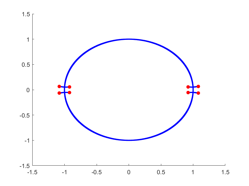
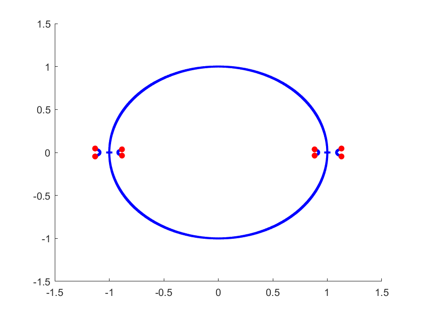
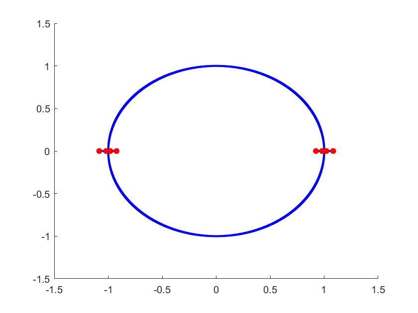
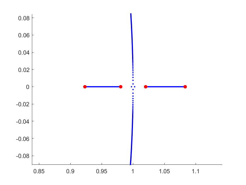
The Lax (Floquet) spectrum of the spectral problem (4.2) for k=0.8k=0.8 and M=20M=20 is shown in Figure 3 on the λ\lambda-plane. The admissible values of λ\lambda are found from invertion of z=λ+λ−1z=\lambda+\lambda^{-1} with two roots

λ=z±z2−42.\lambda=\frac{z\pm\sqrt{z^{2}-4}}{2}. (4.4)

The red dots on the λ\lambda-plane show zeros {±λ1,±λ1−1,±λ2,±λ2−1}\{\pm\lambda_{1},\pm\lambda_{1}^{-1},\pm\lambda_{2},\pm\lambda_{2}^{-1}\} of the polynomial P⁡(λ)P(\lambda) in (3.13) with

ω=dn⁡(α,k)cn2​(α,k)andF1=(1−k2)​sn4​(α,k)cn4​(α,k).\omega=\frac{{\rm dn}(\alpha;k)}{{\rm cn}^{2}(\alpha;k)}\quad\mbox{\rm and}\quad F_{1}=(1-k^{2})\frac{{\rm sn}^{4}(\alpha;k)}{{\rm cn}^{4}(\alpha;k)}. (4.5)

Applying the ordering 0<λ1<λ2<10<\lambda_{1}<\lambda_{2}<1, the two roots λ1\lambda_{1} and λ2\lambda_{2} were obtained in [11] in the explicit form:

λ1=(1−sn⁡(α,k))​(dn⁡(α,k)−1−k2​sn​(α,k))cn⁡(α,k),σ1=−1\lambda_{1}=\frac{\sqrt{\left(1-{\rm sn}(\alpha;k)\right)\left({\rm dn}(\alpha;k)-\sqrt{1-k^{2}}{\rm sn}(\alpha;k)\right)}}{{\rm cn}(\alpha;k)},\quad\sigma_{1}=-1 (4.6)

and

λ2=(1−sn⁡(α,k))​(dn⁡(α,k)+1−k2​sn​(α,k))cn⁡(α,k),σ1=+1.\lambda_{2}=\frac{\sqrt{\left(1-{\rm sn}(\alpha;k)\right)\left({\rm dn}(\alpha;k)+\sqrt{1-k^{2}}{\rm sn}(\alpha;k)\right)}}{{\rm cn}(\alpha;k)},\quad\sigma_{1}=+1. (4.7)

The choice of σ1\sigma_{1} refers to the relation (3.14) when either λ1\lambda_{1} or λ2\lambda_{2} are taken in place of λ1\lambda_{1}. The left panel suggests that the Lax spectrum consists of the unit circle and four segments on the real axis between the eight real roots of P⁡(λ)P(\lambda). The right panel shows the zoomed version to indicate that the spectral bands are connected between the roots.
Refer to caption
Refer to caption
Figure 3. Lax spectrum (left) and its zoom (right) for the dnoidal wave with α=K⁡(k)/M\alpha=K(k)/M with M=20M=20 for k=0.8k=0.8. Red dots show roots of P⁡(λ)P(\lambda).

The left panel of Figure 4 shows the stability spectrum in the Ω\Omega plane, where we recall that Λ\Lambda in the spectral stability problem (3.3) is given by Λ=2​Ω\Lambda=2\Omega in Corollary 1. We relate the values of Ω\Omega and zz by using (3.12)–(3.13) with the substituion z2=λ2+λ−2+2z^{2}=\lambda^{2}+\lambda^{-2}+2. This yields the explicit expression

Ω=±i2​z4−4​(1+ω)​z2+4​(1+2​ω+ω2−F1).\Omega=\pm\frac{i}{2}\sqrt{z^{4}-4(1+\omega)z^{2}+4(1+2\omega+\omega^{2}-F_{1})}. (4.8)

The values of zz are obtained from the Lax spectrum computed numerically from the spectral problem (4.2). Since the stability spectrum include the band on the positive real axis of Ω\Omega, the dnoidal wave is modulationally unstable similar to the constant-amplitude wave in Remark 8.

The right panel of Figure 4 shows Γ:=Ω0/α2\Gamma:=\Omega_{0}/\alpha^{2} versus α\alpha, where Ω0\Omega_{0} is the maximal positive Ω\Omega of the stability spectrum in the Ω\Omega plane. The numerically obtained values are shown by blue dots. The red dashed line shows the constant value 1−k2\sqrt{1-k^{2}} which is the maximal positive Ω\Omega of the dnoidal waves in the continuous NLS equation (1.3) [13]. As k→0k\to 0, this limiting value agrees with the value Ω0=Λ0/2=1\Omega_{0}=\Lambda_{0}/2=1 in Remark 9.

Refer to caption
Refer to caption
Figure 4. Left: Stability spectrum in the Ω\Omega plane for the dnoidal wave with α=K⁡(k)/M\alpha=K(k)/M with M=20M=20 for k=0.8k=0.8. Right: Ω0/α2\Omega_{0}/\alpha^{2} versus parameter α\alpha for fixed k=0.8k=0.8 (dots) and the constant value 1−k2\sqrt{1-k^{2}} (dotted line).

4.3. Cnoidal wave

We set Un=A​cn​(α​n,k)U_{n}=A{\rm cn}(\alpha n;k) according to (2.11) with A=k​sn​(α,k)/dn⁡(α,k)A=k{\rm sn}(\alpha;k)/{\rm dn}(\alpha;k) and look for bounded solutions of the spectral problem (4.2) in the form (4.3). Figure 5 show the Lax spectrum (left) and the stability spectrum (right) for the cnoidal wave with k=0.8k=0.8 (top) and k=0.95k=0.95 (bottom). The red dots on the λ\lambda-plane show again zeros {±λ1,±λ1−1,±λ¯1,±λ¯1−1}\{\pm\lambda_{1},\pm\lambda_{1}^{-1},\pm\bar{\lambda}_{1},\pm\bar{\lambda}_{1}^{-1}\} of the polynomial P⁡(λ)P(\lambda) in (3.13) with

ω=cn⁡(α,k)dn2​(α,k),F1=−k2​(1−k2)​sn4​(α,k)dn4​(α,k).\omega=\frac{{\rm cn}(\alpha;k)}{{\rm dn}^{2}(\alpha;k)},\quad\quad F_{1}=-k^{2}(1-k^{2})\frac{{\rm sn}^{4}(\alpha;k)}{{\rm dn}^{4}(\alpha;k)}. (4.9)

The complex value of λ1\lambda_{1} was obtained in [11] in the explicit form:

λ1=(1−k​sn​(α,k))​(cn⁡(α,k)+i​1−k2​sn​(α,k))dn⁡(α,k),σ1=+1.\lambda_{1}=\frac{\sqrt{(1-k{\rm sn}(\alpha;k))({\rm cn}(\alpha;k)+i\sqrt{1-k^{2}}{\rm sn}(\alpha;k))}}{{\rm dn}(\alpha;k)},\quad\sigma_{1}=+1. (4.10)
Refer to caption
Refer to caption
Refer to caption
Refer to caption
Figure 5. Lax spectrum (left) and stability spectrum on the Ω\Omega plane (right) for the cnoidal wave with α=K⁡(k)/M\alpha=K(k)/M with M=20M=20 for k=0.8k=0.8 (top) and k=0.95k=0.95 (bottom).

The numerical results suggest that the Lax spectrum consists of the unit circle and four complex bands which are either connected across the unit circle for k=0.8k=0.8 or connected away from the unit circle for k=0.95k=0.95. The stability spectrum in both cases displays the figure-eight instability bands in addition to two finite segments along the imaginary axis, boundary of which are beyond the margins of the right panels. The segments on the imaginary axis intersect the figure-eight bands for k=0.8k=0.8 and avoid intersection for k=0.95k=0.95. Because the figure-eight instability bands intersect the origin, the cnoidal wave is also declared to be modulationally unstable with a different instability pattern compared to the dnoidal wave.

We admit that the resolution of numerical data is poor near the origin on the right panels of Figure 5 because resolution of the Lax spectrum is poor near the points ±1\pm 1 on the left panels. It is likely that sensitivity of numerical detected eigenvalues is related to evaluting the square roots in (4.4) and (4.8) near z=±2z=\pm 2.

5. Nonperiodic solutions of linear equaitons

Since the dnoidal and cnoidal waves are modulationally unstable, as is shown in Section 4 based on numerical approximations of the Lax spectrum, we expect the existence of rogue waves (spatially and temporally localized solutions) on the modulationally unstable backgroud. Such solutions were obtained for the continuous NLS equation in [8, 13, 20] and for other related continuous equations in [9, 10, 25, 31].

In order to obtain the rogue waves, as we do in Section 6 by using the analytical theory, we will consider here eigenfunctions of the linear system (3.5)–(3.6) for the eigenvalue λ=λ1\lambda=\lambda_{1} given by a root of the polynomial P⁡(λ)P(\lambda) in (3.13). Since any root of P⁡(λ)P(\lambda) is suitable, this notation for λ1\lambda_{1} is abstract and is not related to the particular choices in (4.6), (4.7), or (4.10).

According to the relations (3.15), the squared eigenfunctions corresponding to the eigenvalue λ=λ1\lambda=\lambda_{1} are periodic. In addition to the periodic eigenfunctions, we construct here the second solution of the linear equations (3.5)–(3.6) which are unbounded both in n∈ℤn\in\mathbb{Z} and t∈ℝt\in\mathbb{R}.

The following lemma gives a construction of the second solution of the linear equations (3.5)–(3.6) for an eigenvalue λ=λ1\lambda=\lambda_{1}.

Lemma 5.

Let {(Pn​(t),Qn​(t))T}n∈ℤ\{(P_{n}(t),Q_{n}(t))^{\mathrm{T}}\}_{n\in\mathbb{Z}} be the eigenfunction of the linear system (3.5)–(3.6) for an eigenvalue λ=λ1\lambda=\lambda_{1}. The second solution {(P^n​(t),Q^n​(t))T}n∈ℤ\{(\hat{P}_{n}(t),\hat{Q}_{n}(t))^{\mathrm{T}}\}_{n\in\mathbb{Z}} of the linear system (3.5)–(3.6) for the same eigenvalue λ=λ1\lambda=\lambda_{1} can be represented in the form

P^n​(t)=Pn​(t)​θn​(t)−Q¯n​(t)|Pn​(t)|2+|Qn​(t)|2,Q^n​(t)=Qn​(t)​θn​(t)+P¯n​(t)|Pn​(t)|2+|Qn​(t)|2,\hat{P}_{n}(t)=P_{n}(t)\theta_{n}(t)-\frac{\bar{Q}_{n}(t)}{|P_{n}(t)|^{2}+|Q_{n}(t)|^{2}},\quad\hat{Q}_{n}(t)=Q_{n}(t)\theta_{n}(t)+\frac{\bar{P}_{n}(t)}{|P_{n}(t)|^{2}+|Q_{n}(t)|^{2}}, (5.1)

where θn​(t)\theta_{n}(t) is a solution of the linear equations

θn+1−θn=(|λ1|2−1)​(λ¯1​Un​P¯n2−λ1​U¯n​Q¯n2−(1+|λ1|2)​P¯n​Q¯n)(|Pn|2+|Qn|2)​Δn\theta_{n+1}-\theta_{n}=\frac{(|\lambda_{1}|^{2}-1)(\bar{\lambda}_{1}U_{n}\bar{P}_{n}^{2}-\lambda_{1}\bar{U}_{n}\bar{Q}_{n}^{2}-(1+|\lambda_{1}|^{2})\bar{P}_{n}\bar{Q}_{n})}{(|P_{n}|^{2}+|Q_{n}|^{2})\Delta_{n}} (5.2)

and

d​θnd​t\displaystyle\frac{d\theta_{n}}{dt} =i⁡(|λ1|2−1)​Σn|λ1|2​(|Pn|2+|Qn|2)2\displaystyle=\frac{i(|\lambda_{1}|^{2}-1)\Sigma_{n}}{|\lambda_{1}|^{2}(|P_{n}|^{2}+|Q_{n}|^{2})^{2}} (5.3)

with

Δn\displaystyle\Delta_{n} :=|λ1|4​|Pn|2+|Qn|2+|λ1|2​|Un|2​(|Pn|2+|Qn|2)+(|λ1|2−1)​(λ¯1​Un​P¯n​Qn+λ1​U¯n​Pn​Q¯n),\displaystyle:=|\lambda_{1}|^{4}|P_{n}|^{2}+|Q_{n}|^{2}+|\lambda_{1}|^{2}|U_{n}|^{2}(|P_{n}|^{2}+|Q_{n}|^{2})+(|\lambda_{1}|^{2}-1)(\bar{\lambda}_{1}U_{n}\bar{P}_{n}Q_{n}+\lambda_{1}\bar{U}_{n}P_{n}\bar{Q}_{n}),
Σn\displaystyle\Sigma_{n} :=(λ1​Un+λ¯1​Un−1)​P¯n2+(λ¯1​U¯n+λ1​U¯n−1)​Q¯n2−(1+|λ1|−2)​(λ12−λ¯12)​P¯n​Q¯n.\displaystyle:=(\lambda_{1}U_{n}+\bar{\lambda}_{1}U_{n-1})\bar{P}_{n}^{2}+(\bar{\lambda}_{1}\bar{U}_{n}+\lambda_{1}\bar{U}_{n-1})\bar{Q}_{n}^{2}-(1+|\lambda_{1}|^{-2})(\lambda_{1}^{2}-\bar{\lambda}_{1}^{2})\bar{P}_{n}\bar{Q}_{n}.
Proof.

We obtain from (3.5) that

|Pn+1|2+|Qn+1|2=|λ1​Pn+Un​Qn|2+|λ1−1​Qn−U¯n​Pn|21+|Un|2.\displaystyle|P_{n+1}|^{2}+|Q_{n+1}|^{2}=\frac{|\lambda_{1}P_{n}+U_{n}Q_{n}|^{2}+|\lambda_{1}^{-1}Q_{n}-\bar{U}_{n}P_{n}|^{2}}{1+|U_{n}|^{2}}. (5.4)

If (Pn,Qn)T(P_{n},Q_{n})^{\mathrm{T}} and (P^n,Q^n)T(\hat{P}_{n},\hat{Q}_{n})^{\mathrm{T}} satisfy the linear equation (3.5), then expression (5.1) implies that {θn}n∈ℤ\{\theta_{n}\}_{n\in\mathbb{Z}} is a solution of

(λ1​Pn+Un​Qn)​(θn+1−θn)=Un​P¯n−λ1​Q¯n|Pn|2+|Qn|2−Un​P¯n−λ¯1−1​Q¯n|Pn+1|2+|Qn+1|2.\displaystyle(\lambda_{1}P_{n}+U_{n}Q_{n})(\theta_{n+1}-\theta_{n})=\frac{U_{n}\bar{P}_{n}-\lambda_{1}\bar{Q}_{n}}{|P_{n}|^{2}+|Q_{n}|^{2}}-\frac{U_{n}\bar{P}_{n}-\bar{\lambda}_{1}^{-1}\bar{Q}_{n}}{|P_{n+1}|^{2}+|Q_{n+1}|^{2}}.

Substituting (5.4) and dividing by (λ1​Pn+Un​Qn)(\lambda_{1}P_{n}+U_{n}Q_{n}) yield (5.2) after simplifications.

We obtain from (3.6) that

dd​t​(|Pn|2+|Qn|2)\displaystyle\frac{d}{dt}(|P_{n}|^{2}+|Q_{n}|^{2}) =i⁡(Wn−W¯n)​(|Pn|2−|Qn|2)\displaystyle=i(W_{n}-\bar{W}_{n})(|P_{n}|^{2}-|Q_{n}|^{2})
+i⁡[(λ1−λ¯1−1)​Un+(λ¯1−λ1−1)​Un−1]​P¯n​Qn\displaystyle\quad+i\left[(\lambda_{1}-\bar{\lambda}_{1}^{-1})U_{n}+(\bar{\lambda}_{1}-{\lambda}_{1}^{-1})U_{n-1}\right]\bar{P}_{n}Q_{n}
−i⁡[(λ¯1−λ1−1)​U¯n+(λ1−λ¯1−1)​U¯n−1]​Pn​Q¯n.\displaystyle\quad-i\left[(\bar{\lambda}_{1}-{\lambda}_{1}^{-1})\bar{U}_{n}+(\lambda_{1}-\bar{\lambda}_{1}^{-1})\bar{U}_{n-1}\right]P_{n}\bar{Q}_{n}. (5.5)

If (Pn,Qn)T(P_{n},Q_{n})^{\mathrm{T}} and (P^n,Q^n)T(\hat{P}_{n},\hat{Q}_{n})^{\mathrm{T}} satisfy the linear equation (3.6), then substituting (5.1) and (5.5) into (3.6) and dividing by PnP_{n} yield (5.3) after simplifications. ∎

Remark 10.

The result of Lemma 5 does not use the relations (3.15). In other words, λ1\lambda_{1} in Lemma 5 does not have to be a root of P⁡(λ)P(\lambda) in (3.13).

If we use the relations (3.15) as in Remark 10, then we can simplify the relations (5.2) and (5.3). This is done separately for the case of dnoidal and cnoidal waves. The following lemma summarizes the results of these computations.

Lemma 6.

Let {Un}n∈ℤ\{U_{n}\}_{n\in\mathbb{Z}} be either the dnoidal or cnoidal waves given by (2.8) or (2.11) and λ1\lambda_{1} be a root of the polynomial P⁡(λ)P(\lambda) in (3.13). Then, θn​(t)=Θn+i​t\theta_{n}(t)=\Theta_{n}+it in the representation (5.1) with {Θn}n∈ℤ\{\Theta_{n}\}_{n\in\mathbb{Z}} being a time-independent solution of the difference equations:

θn+1−θn=(λ1+λ1−1)​(|Un|2−σ1​F1)(λ1−λ1−1)​(F1+2​(1+ω)​|Un|2+|Un|4)\theta_{n+1}-\theta_{n}=\frac{(\lambda_{1}+{\lambda}_{1}^{-1})(|U_{n}|^{2}-\sigma_{1}\sqrt{F_{1}})}{(\lambda_{1}-\lambda_{1}^{-1})(F_{1}+2(1+\omega)|U_{n}|^{2}+|U_{n}|^{4})} (5.6)

or

θn+1−θn=(|λ1|2−1)​(λ¯1​λ1−1+λ¯1−2)​|Un|2+F1​(|λ1|2−|λ1|−2)Γn,\theta_{n+1}-\theta_{n}=\frac{(|\lambda_{1}|^{2}-1)(\bar{\lambda}_{1}\lambda_{1}^{-1}+\bar{\lambda}_{1}^{-2})|U_{n}|^{2}+\sqrt{F_{1}}(|\lambda_{1}|^{2}-|\lambda_{1}|^{-2})}{\Gamma_{n}}, (5.7)

with

Γn\displaystyle\Gamma_{n} =|Un|2​(|λ1|4+|λ1|−4+2​|Un−1|2−2​|Un|2)+2​|Un−1|2\displaystyle=|U_{n}|^{2}\Big(|\lambda_{1}|^{4}+|\lambda_{1}|^{-4}+2|U_{n-1}|^{2}-2|U_{n}|^{2}\Big)+2|U_{n-1}|^{2}
+(|λ1|2+|λ1|−2)​(|Un|4−F1−λ¯1​λ1−1​U¯n​Un−1−λ1​λ¯1−1​Un​U¯n−1)\displaystyle\quad+(|\lambda_{1}|^{2}+|\lambda_{1}|^{-2})\Big(|U_{n}|^{4}-F_{1}-\bar{\lambda}_{1}\lambda_{1}^{-1}\bar{U}_{n}U_{n-1}-\lambda_{1}\bar{\lambda}_{1}^{-1}U_{n}\bar{U}_{n-1}\Big)

where (5.6) and (5.7) correspond to the dnoidal or cnoidal waves respectively.

Proof.

For the cnoidal wave, we assume that λ1∈ℂ\lambda_{1}\in\mathbb{C} is given by (4.10), whereas ω>0\omega>0 and F1<0F_{1}<0 are given by (4.9). It follows from (3.14) with σ1=1\sigma_{1}=1 and F1<0F_{1}<0 that

λ12+λ1−2+λ¯12+λ¯1−2=4​ω,λ12+λ1−2−λ¯12−λ¯1−2=−4​F1.\begin{array}[]{l}\lambda_{1}^{2}+\lambda_{1}^{-2}+\bar{\lambda}_{1}^{2}+\bar{\lambda}_{1}^{-2}=4\omega,\\ \lambda_{1}^{2}+\lambda_{1}^{-2}-\bar{\lambda}_{1}^{2}-\bar{\lambda}_{1}^{-2}=-4\sqrt{F_{1}}.\\ \end{array} (5.8)

It follows from (3.15) with σ1=1\sigma_{1}=1, F0=0F_{0}=0, and F1<0F_{1}<0 that

(|Pn|2+|Qn|2)2\displaystyle(|P_{n}|^{2}+|Q_{n}|^{2})^{2} =|λ1​Un−λ1−1​Un−1|2+|λ1​U¯n−1−λ1−1​U¯n|2+12​(Un​U¯n−1+U¯n​Un−1)2−2​F1\displaystyle=|\lambda_{1}U_{n}-\lambda_{1}^{-1}U_{n-1}|^{2}+|\lambda_{1}\bar{U}_{n-1}-\lambda_{1}^{-1}\bar{U}_{n}|^{2}+\frac{1}{2}(U_{n}\bar{U}_{n-1}+\bar{U}_{n}U_{n-1})^{2}-2F_{1}
=(|λ1|2+|λ1|−2)​(|Un|2+|Un−1|2)−2​λ1−1​λ¯1​U¯n​Un−1−2​λ1​λ¯1−1​Un​U¯n−1\displaystyle=(|\lambda_{1}|^{2}+|\lambda_{1}|^{-2})(|U_{n}|^{2}+|U_{n-1}|^{2})-2\lambda_{1}^{-1}\bar{\lambda}_{1}\bar{U}_{n}U_{n-1}-2\lambda_{1}\bar{\lambda}_{1}^{-1}U_{n}\bar{U}_{n-1}
+2​|Un|2​|Un−1|2−2​F1.\displaystyle\quad+2|U_{n}|^{2}|U_{n-1}|^{2}-2F_{1}.

Similarly, we obtain from (3.15) that

(1−|λ1|−2)​Σn\displaystyle(1-|\lambda_{1}|^{-2})\Sigma_{n} =(|λ1|2−2+|λ1|−2)​(|Un|2+|Un−1|2)+2​λ¯1​(λ¯1−λ1−1)​U¯n​Un−1\displaystyle=(|\lambda_{1}|^{2}-2+|\lambda_{1}|^{-2})(|U_{n}|^{2}+|U_{n-1}|^{2})+2\bar{\lambda}_{1}(\bar{\lambda}_{1}-\lambda_{1}^{-1})\bar{U}_{n}U_{n-1}
+2​λ¯1−1​(λ¯1−1−λ1)​Un​U¯n−1+12​(λ12+λ1−2−λ¯12−λ¯1−2)​(Un​U¯n−1+U¯n​Un−1+2​F1),\displaystyle\quad+2\bar{\lambda}_{1}^{-1}(\bar{\lambda}_{1}^{-1}-\lambda_{1})U_{n}\bar{U}_{n-1}+\frac{1}{2}(\lambda_{1}^{2}+\lambda_{1}^{-2}-\bar{\lambda}_{1}^{2}-\bar{\lambda}_{1}^{-2})(U_{n}\bar{U}_{n-1}+\bar{U}_{n}U_{n-1}+2\sqrt{F_{1}}),

where we have used that F1∈i​ℝ\sqrt{F_{1}}\in i\mathbb{R}. By using F0=0F_{0}=0 and (5.8), we can simplify the previous expression to the form:

(1−|λ1|−2)​Σn\displaystyle(1-|\lambda_{1}|^{-2})\Sigma_{n} =(|λ1|2−2+|λ1|−2)​(|Un|2+|Un−1|2)−2​λ¯1​λ1−1​U¯n​Un−1−2​λ¯1−1​λ1​Un​U¯n−1\displaystyle=(|\lambda_{1}|^{2}-2+|\lambda_{1}|^{-2})(|U_{n}|^{2}+|U_{n-1}|^{2})-2\bar{\lambda}_{1}\lambda_{1}^{-1}\bar{U}_{n}U_{n-1}-2\bar{\lambda}_{1}^{-1}\lambda_{1}U_{n}\bar{U}_{n-1}
+12​(λ12+λ1−2−λ¯12−λ¯1−2)​(Un​U¯n−1+U¯n​Un−1+2​F1)\displaystyle\quad+\frac{1}{2}(\lambda_{1}^{2}+\lambda_{1}^{-2}-\bar{\lambda}_{1}^{2}-\bar{\lambda}_{1}^{-2})(U_{n}\bar{U}_{n-1}+\bar{U}_{n}U_{n-1}+2\sqrt{F_{1}})
=(|λ1|2−2+|λ1|−2)​(|Un|2+|Un−1|2)−2​λ¯1​λ1−1​U¯n​Un−1−2​λ¯1−1​λ1​Un​U¯n−1\displaystyle=(|\lambda_{1}|^{2}-2+|\lambda_{1}|^{-2})(|U_{n}|^{2}+|U_{n-1}|^{2})-2\bar{\lambda}_{1}\lambda_{1}^{-1}\bar{U}_{n}U_{n-1}-2\bar{\lambda}_{1}^{-1}\lambda_{1}U_{n}\bar{U}_{n-1}
+2​ω​(Un​U¯n−1+U¯n​Un−1)−4​F1.\displaystyle\quad+2\omega(U_{n}\bar{U}_{n-1}+\bar{U}_{n}U_{n-1})-4F_{1}.

Due to the conservation (2.7), this implies that (1−|λ1|−2)​Σn=(|Pn|2+|Qn|2)2(1-|\lambda_{1}|^{-2})\Sigma_{n}=(|P_{n}|^{2}+|Q_{n}|^{2})^{2} and hence (5.3) becomes a trivial equation θ˙n=i\dot{\theta}_{n}=i, with the solution θn​(t)=Θn+i​t\theta_{n}(t)=\Theta_{n}+it, where Θn\Theta_{n} is tt-independent. To get {Θn}n∈ℤ\{\Theta_{n}\}_{n\in\mathbb{Z}}, we substitute (3.15) into (5.2) and simplify the result with a lengthy but direct computation to the form (5.7), where we have used that σ1=1\sigma_{1}=1, F0=0F_{0}=0, and F1∈i​ℝ\sqrt{F_{1}}\in i\mathbb{R}.

For the dnoidal wave, we assume that λ1∈ℝ\lambda_{1}\in\mathbb{R} is given by either (4.6) or (4.7), whereas ω>0\omega>0 and F1>0F_{1}>0 are given by (4.5). Without loss of generality, we consider (4.6) with σ1=−1\sigma_{1}=-1. It follows from (3.15) with σ1=−1\sigma_{1}=-1 that

(|Pn|2+|Qn|2)2\displaystyle(|P_{n}|^{2}+|Q_{n}|^{2})^{2} =(λ12+λ1−2)​(|Un|2+|Un−1|2)+12​(Un​U¯n−1+U¯n​Un−1+2​F1)2\displaystyle=({\lambda}_{1}^{2}+{\lambda}_{1}^{-2})(|U_{n}|^{2}+|U_{n-1}|^{2})+\frac{1}{2}(U_{n}\bar{U}_{n-1}+\bar{U}_{n}U_{n-1}+2\sqrt{F_{1}})^{2}
−2​(Un​U¯n−1+U¯n​Un−1)\displaystyle\quad\quad-2(U_{n}\bar{U}_{n-1}+\bar{U}_{n}U_{n-1})
=(λ12+λ1−2−2)​(U¯n​Un−1+Un​U¯n−1+|Un|2+|Un−1|2)\displaystyle=(\lambda_{1}^{2}+\lambda_{1}^{-2}-2)(\bar{U}_{n}U_{n-1}+U_{n}\bar{U}_{n-1}+|U_{n}|^{2}+|U_{n-1}|^{2})

and

(1−λ1−2)​Σn\displaystyle(1-\lambda_{1}^{-2})\Sigma_{n} =(λ12+λ1−2−2)​(|Un|2+|Un−1|2)+2​(λ12−1)​U¯n​Un−1−2​(1−λ1−2)​Un​U¯n−1\displaystyle=({\lambda}_{1}^{2}+\lambda_{1}^{-2}-2)(|U_{n}|^{2}+|U_{n-1}|^{2})+2(\lambda_{1}^{2}-1)\bar{U}_{n}U_{n-1}-2(1-\lambda_{1}^{-2})U_{n}\bar{U}_{n-1}
=(λ12+λ1−2−2)​(U¯n​Un−1+Un​U¯n−1+|Un|2+|Un−1|2),\displaystyle=(\lambda_{1}^{2}+\lambda_{1}^{-2}-2)(\bar{U}_{n}U_{n-1}+U_{n}\bar{U}_{n-1}+|U_{n}|^{2}+|U_{n-1}|^{2}),

where we have used (2.6) and (2.7) with F0=0F_{0}=0 and F1>0F_{1}>0 and (3.14) with σ1=−1\sigma_{1}=-1. Thus, we have (1−λ1−2)​Σ=(|Pn|2+|Qn|2)2(1-\lambda_{1}^{-2})\Sigma=(|P_{n}|^{2}+|Q_{n}|^{2})^{2} so that (5.3) becomes again a trivial equation θ˙n=i\dot{\theta}_{n}=i. Again, we have θn​(t)=Θn+i​t\theta_{n}(t)=\Theta_{n}+it, where the tt-independent Θn\Theta_{n} is obtained from the difference equation (5.2). After long but straightforward computations, we have simplified the expression to the form (5.6), where we have used (3.14) and restored the value of σ1\sigma_{1} for either (4.6) or (4.7). ∎

6. Construction of rogue waves

Here we construct the rogue waves on the background of the standing periodic waves. To do so, we use the one-fold Darboux transformation (11-fold DT). The 11-fold DT has already been constructed for the AL equation (1.1) in [26] but the formulas used eigenfunctions of the Lax system (2.2)–(2.3), which is not suitable for the standing periodic waves as in Remark 1. Therefore, our first task is to extend the 11-fold DT to the eigenfunctions of the Lax system (2.1). We achieve the task with direct computations similarly to computations in [37] and [11].

The following lemma presents the 11-fold DT for the AL equation (1.1) in terms of solutions of the linear system (2.2).

Lemma 7.

Let {un​(t)}n∈ℤ\{u_{n}(t)\}_{n\in\mathbb{Z}} be a solution of the AL equation (1.1), {(pn​(t),qn​(t))T}n∈ℤ\{(p_{n}(t),q_{n}(t))^{\mathrm{T}}\}_{n\in\mathbb{Z}} be a nontrivial solution to the linear system (2.1) with λ=λ1\lambda=\lambda_{1}, and {φn​(t)}n∈ℤ\{\varphi_{n}(t)\}_{n\in\mathbb{Z}} be any solution to the linear system (2.1) with arbitrary λ∈ℂ\lambda\in\mathbb{C}. Then, {u^n​(t)}n∈ℤ\{\hat{u}_{n}(t)\}_{n\in\mathbb{Z}} given by

u^n=−λ1​(|pn|2+|λ1|2​|qn|2)λ¯1​(|λ1|2​|pn|2+|qn|2)​un+λ1​(1−|λ1|4)​pn​q¯nλ¯12​(|λ1|2​|pn|2+|qn|2)\hat{u}_{n}=-\frac{\lambda_{1}(|p_{n}|^{2}+|\lambda_{1}|^{2}|q_{n}|^{2})}{\bar{\lambda}_{1}(|\lambda_{1}|^{2}|p_{n}|^{2}+|q_{n}|^{2})}u_{n}+\frac{\lambda_{1}(1-|\lambda_{1}|^{4})p_{n}\bar{q}_{n}}{\bar{\lambda}_{1}^{2}(|\lambda_{1}|^{2}|p_{n}|^{2}+|q_{n}|^{2})} (6.1)

is a new solution of the AL equation (1.1) and {φ^n​(t)}n∈ℤ\{\hat{\varphi}_{n}(t)\}_{n\in\mathbb{Z}} given by φ^n=Mn​(λ)​φn\hat{\varphi}_{n}=M_{n}(\lambda)\varphi_{n} is a new solution to the linear system (2.1) with arbitrary λ\lambda, where

Mn​(λ)=|pn|2+|λ1|2​|qn|2|λ1|2​|pn|2+|qn|2​(λ+λ−1​anbn−b¯nλ​a¯n+λ−1)M_{n}(\lambda)=\frac{\sqrt{|p_{n}|^{2}+|\lambda_{1}|^{2}|q_{n}|^{2}}}{\sqrt{|\lambda_{1}|^{2}|p_{n}|^{2}+|q_{n}|^{2}}}\left(\begin{array}[]{cc}\lambda+\lambda^{-1}a_{n}&b_{n}\\ -\bar{b}_{n}&\lambda\bar{a}_{n}+\lambda^{-1}\end{array}\right)

with

an=−λ1​(|λ1|2​|pn|2+|qn|2)λ¯1​(|pn|2+|λ1|2​|qn|2),bn=λ1​(1−|λ1|4)​pn​q¯n|λ1|2​(|pn|2+|λ1|2​|qn|2).a_{n}=-\frac{\lambda_{1}(|\lambda_{1}|^{2}|p_{n}|^{2}+|q_{n}|^{2})}{\bar{\lambda}_{1}(|p_{n}|^{2}+|\lambda_{1}|^{2}|q_{n}|^{2})},\qquad b_{n}=\frac{\lambda_{1}(1-|\lambda_{1}|^{4})p_{n}\bar{q}_{n}}{|\lambda_{1}|^{2}(|p_{n}|^{2}+|\lambda_{1}|^{2}|q_{n}|^{2})}.
Proof.

We need to show validity of the Darboux equations

U⁡(u^n,λ)​Mn​(λ)=Mn+1​(λ)​U​(un,λ){U}(\hat{u}_{n},\lambda)M_{n}(\lambda)=M_{n+1}(\lambda){U}(u_{n},\lambda) (6.2)

and

V⁡(u^n,λ)​Mn​(λ)=M˙n​(λ)+Mn​(λ)​V​(un,λ).V(\hat{u}_{n},\lambda)M_{n}(\lambda)=\dot{M}_{n}(\lambda)+M_{n}(\lambda)V(u_{n},\lambda). (6.3)

Substituting U⁡(un,λ)U(u_{n},\lambda) and Mn​(λ)M_{n}(\lambda) into (6.2) and collecting different powers with respect to λ\lambda yields the system of equations

{a¯n​u^n+bn−un=0,u^n−an+1​un−bn+1=0,an+1−an−bn+1​u¯n+b¯n​u^n=0,an+1​(1+un2)−an​(1+u^n2)=0.\left\{\begin{array}[]{l}\bar{a}_{n}\hat{u}_{n}+b_{n}-u_{n}=0,\\ \hat{u}_{n}-a_{n+1}u_{n}-b_{n+1}=0,\\ a_{n+1}-a_{n}-b_{n+1}\bar{u}_{n}+\bar{b}_{n}\hat{u}_{n}=0,\\ a_{n+1}(1+u_{n}^{2})-a_{n}(1+\hat{u}_{n}^{2})=0.\end{array}\right. (6.4)

It follows from φn+1=U⁡(un,λ)​φn\varphi_{n+1}=U(u_{n},\lambda)\varphi_{n} that

|pn+1|2+|λ1|2​|qn+1|2=|λ1|2​|pn|2+|qn|2,\displaystyle|p_{n+1}|^{2}+|\lambda_{1}|^{2}|q_{n+1}|^{2}=|\lambda_{1}|^{2}|p_{n}|^{2}+|q_{n}|^{2},
(1+|un|2)​(|λ1|2​|pn+1|2+|qn+1|2)\displaystyle(1+|u_{n}|^{2})(|\lambda_{1}|^{2}|p_{n+1}|^{2}+|q_{n+1}|^{2}) =(|λ1|2+|un|2)​|pn|2+un​p¯n​qn​(λ¯1​|λ1|2−λ1−1)\displaystyle=(|\lambda_{1}|^{2}+|u_{n}|^{2})|p_{n}|^{2}+u_{n}\bar{p}_{n}q_{n}(\bar{\lambda}_{1}|\lambda_{1}|^{2}-\lambda_{1}^{-1})
+u¯n​pn​q¯n​(λ1​|λ1|2−λ¯1−1)+(|λ1|2​|un|2+|λ1|−2)​|qn|2,\displaystyle\quad+\bar{u}_{n}p_{n}\bar{q}_{n}(\lambda_{1}|\lambda_{1}|^{2}-\bar{\lambda}_{1}^{-1})+(|\lambda_{1}|^{2}|u_{n}|^{2}+|\lambda_{1}|^{-2})|q_{n}|^{2},

and

(1+|un|2)​pn+1​q¯n+1\displaystyle(1+|u_{n}|^{2})p_{n+1}\bar{q}_{n+1} =−λ1​un​|pn|2+λ1​λ¯1−1​pn​q¯n−un2​p¯n​qn+λ¯1−1​un​|qn|2.\displaystyle=-\lambda_{1}u_{n}|p_{n}|^{2}+\lambda_{1}\bar{\lambda}_{1}^{-1}p_{n}\bar{q}_{n}-u_{n}^{2}\bar{p}_{n}q_{n}+\bar{\lambda}_{1}^{-1}u_{n}|q_{n}|^{2}.

By using the previous expressions and the definitions of ana_{n} and bnb_{n}, we have verified that the first two equations in system (6.4) are equivalent to each other and yield the transformation formula (6.1). The third equation in system (6.4) transforms to the relation

|an|2+|bn|2−a¯n​an+1+u¯n​a¯n​bn+1−un​b¯n=0,|a_{n}|^{2}+|b_{n}|^{2}-\bar{a}_{n}a_{n+1}+\bar{u}_{n}\bar{a}_{n}b_{n+1}-u_{n}\bar{b}_{n}=0,

which holds true after straightforward computations. Finally, the fourth equation in system (6.4) is consistent with the first three equations after substitutions.

Substituting V⁡(un,λ)V(u_{n},\lambda) and Mn​(λ)M_{n}(\lambda) into (6.3) and collecting different powers with respect to λ\lambda yields the system of equations

{a¯n​u^n+bn−un=0,u^n−1−an​un−1−bn=0,a˙n−i​an​(un​u¯n−1+u¯n​un−1−u^n​u^¯n−1−u^¯n​u^n−1−2​bn​u¯n−1+2​b¯n​u^n)=0,a˙n−i⁡[an​(u^n​u^¯n−1+u^¯n​u^n−1−un​u¯n−1−u¯n​un−1)+2​b¯n​u^n−1−2​bn​u¯n]=0,b˙n−i⁡[(1+|bn|2)​u^n+bn​(un​u¯n−1+u¯n​un−1)−bn2​u¯n−1−a¯n​u^n−1−an​un+un−1]=0.\left\{\begin{array}[]{l}\bar{a}_{n}\hat{u}_{n}+b_{n}-u_{n}=0,\\ \hat{u}_{n-1}-a_{n}u_{n-1}-b_{n}=0,\\ \dot{a}_{n}-ia_{n}\left(u_{n}\bar{u}_{n-1}+\bar{u}_{n}u_{n-1}-\hat{u}_{n}\bar{\hat{u}}_{n-1}-\bar{\hat{u}}_{n}\hat{u}_{n-1}-2b_{n}\bar{u}_{n-1}+2\bar{b}_{n}\hat{u}_{n}\right)=0,\\ \dot{a}_{n}-i\left[a_{n}(\hat{u}_{n}\bar{\hat{u}}_{n-1}+\bar{\hat{u}}_{n}\hat{u}_{n-1}-u_{n}\bar{u}_{n-1}-\bar{u}_{n}u_{n-1})+2\bar{b}_{n}\hat{u}_{n-1}-2b_{n}\bar{u}_{n}\right]=0,\\ \dot{b}_{n}-i\left[(1+|b_{n}|^{2})\hat{u}_{n}+b_{n}(u_{n}\bar{u}_{n-1}+\bar{u}_{n}u_{n-1})-b_{n}^{2}\bar{u}_{n-1}-\bar{a}_{n}\hat{u}_{n-1}-a_{n}u_{n}+u_{n-1}\right]=0.\end{array}\right. (6.5)

It is obvious that the first two equations in system (6.5) repeat the first two equations in system (6.4), while the third and the fourth equations in system (6.5) are identical to each other. The third and fifth equations in system (6.5) are further reduced to the form:

a˙n=i⁡[λ12​λ¯1−2​b¯n​(un−bn)+an​(un−1​b¯n−bn​u¯n−1)−bn​(u¯n−b¯n)],\dot{a}_{n}=i\left[\lambda_{1}^{2}\bar{\lambda}_{1}^{-2}\bar{b}_{n}(u_{n}-b_{n})+a_{n}(u_{n-1}\bar{b}_{n}-b_{n}\bar{u}_{n-1})-b_{n}(\bar{u}_{n}-\bar{b}_{n})\right],

and

b˙n\displaystyle\dot{b}_{n} =i[a¯n−1(1+|bn|2)(un−bn)+bn(unu¯n−1+u¯nun−1)\displaystyle=i[\bar{a}_{n}^{-1}(1+|b_{n}|^{2})(u_{n}-b_{n})+b_{n}(u_{n}\bar{u}_{n-1}+\bar{u}_{n}u_{n-1})
−(1+|an|2)un−1−bn2u¯n−1−anun−a¯nbn].\displaystyle\quad-(1+|a_{n}|^{2})u_{n-1}-b_{n}^{2}\bar{u}_{n-1}-a_{n}u_{n}-\bar{a}_{n}b_{n}].

It follows from φ˙n=V⁡(un,λ)​φn\dot{\varphi}_{n}=V(u_{n},\lambda)\varphi_{n} that

dd​t​(|λ1|2​|pn|2+|qn|2)\displaystyle\frac{d}{dt}(|\lambda_{1}|^{2}|p_{n}|^{2}+|q_{n}|^{2}) =i2​(λ12+λ1−2−λ¯12−λ¯1−2)​(|λ1|2​|pn|2−|qn|2)\displaystyle=\frac{i}{2}(\lambda_{1}^{2}+\lambda_{1}^{-2}-\bar{\lambda}_{1}^{2}-\bar{\lambda}_{1}^{-2})(|\lambda_{1}|^{2}|p_{n}|^{2}-|q_{n}|^{2})
+i⁡(|λ1|4−1)​(λ¯1−1​un​p¯n​qn−λ1−1​u¯n​pn​q¯n),\displaystyle\quad+i(|\lambda_{1}|^{4}-1)(\bar{\lambda}_{1}^{-1}u_{n}\bar{p}_{n}q_{n}-\lambda_{1}^{-1}\bar{u}_{n}p_{n}\bar{q}_{n}),
dd​t​(|pn|2+|λ1|2​|qn|2)\displaystyle\frac{d}{dt}(|p_{n}|^{2}+|\lambda_{1}|^{2}|q_{n}|^{2}) =i2​(λ12+λ1−2−λ¯12−λ¯1−2)​(|pn|2−|λ1|2​|qn|2)\displaystyle=\frac{i}{2}(\lambda_{1}^{2}+\lambda_{1}^{-2}-\bar{\lambda}_{1}^{2}-\bar{\lambda}_{1}^{-2})(|p_{n}|^{2}-|\lambda_{1}|^{2}|q_{n}|^{2})
+i⁡(|λ1|4−1)​(λ1−1​un−1​p¯n​qn−λ¯1−1​u¯n−1​pn​q¯n),\displaystyle\quad+i(|\lambda_{1}|^{4}-1)(\lambda_{1}^{-1}u_{n-1}\bar{p}_{n}q_{n}-\bar{\lambda}_{1}^{-1}\bar{u}_{n-1}p_{n}\bar{q}_{n}),

and

dd​t​(pn​q¯n)\displaystyle\frac{d}{dt}(p_{n}\bar{q}_{n}) =i⁡(λ¯1​un−1−λ¯1−1​un)​|pn|2+i⁡(λ1​un−λ1−1​un−1)​|qn|2\displaystyle=i(\bar{\lambda}_{1}u_{n-1}-\bar{\lambda}_{1}^{-1}u_{n})|p_{n}|^{2}+i(\lambda_{1}u_{n}-\lambda_{1}^{-1}u_{n-1})|q_{n}|^{2}
OPEN+i2​(λ12+λ1−2+λ¯12+λ¯1−2+2​(un​u¯n−1+u¯n​un−1))​pn​q¯n).\displaystyle\quad+\frac{i}{2}(\lambda_{1}^{2}+\lambda_{1}^{-2}+\bar{\lambda}_{1}^{2}+\bar{\lambda}_{1}^{-2}+2(u_{n}\bar{u}_{n-1}+\bar{u}_{n}u_{n-1}))p_{n}\bar{q}_{n}).

We have verified with the help of the Wolfram’s Mathematica that the two equations for a˙n\dot{a}_{n} and b˙n\dot{b}_{n} are satisfied by using the previous expressions and the definitions of ana_{n} and bnb_{n}. ∎

The following two remarks report applications of the 11-fold DT with the periodic eigenfunctions of the dnoidal and cnoidal waves. As expected from similar applications in [8, 13], the 11-fold DT recovers the same dnoidal and cnoidal waves after translations in space and complex phase.

Remark 11.

Let {un​(t)}n∈ℤ\{u_{n}(t)\}_{n\in\mathbb{Z}} be the dnoidal wave in the form (2.4) and (2.8), and {(pn​(t),qn​(t))T}n∈ℤ\{(p_{n}(t),q_{n}(t))^{\mathrm{T}}\}_{n\in\mathbb{Z}} be the eigenfunction of the linear system (2.1) associated with λ=λ1\lambda=\lambda_{1} in the form (3.4) and (3.15). Since UnU_{n} and λ1\lambda_{1} are real, the 1-fold DT (6.1) yields

u^n\displaystyle\hat{u}_{n} =[−|Pn|2+λ12​|Qn|2λ12​|Pn|2+|Qn|2​Un−(λ13−λ1−1)​Pn​Q¯nλ12​|Pn|2+|Qn|2]​e2​i​ω​t\displaystyle=\left[-\frac{|P_{n}|^{2}+\lambda_{1}^{2}|Q_{n}|^{2}}{\lambda_{1}^{2}|P_{n}|^{2}+|Q_{n}|^{2}}U_{n}-\frac{(\lambda_{1}^{3}-\lambda_{1}^{-1})P_{n}\bar{Q}_{n}}{\lambda_{1}^{2}|P_{n}|^{2}+|Q_{n}|^{2}}\right]e^{2i\omega t}
=−σ1​F1Un​e2​i​ω​t,\displaystyle=-\frac{\sigma_{1}\sqrt{F_{1}}}{U_{n}}e^{2i\omega t},

where we have used (3.15) after multiplying the numerator and the denominator by P¯n​Qn\bar{P}_{n}Q_{n}. By using (2.8) and (4.5), we obtain

u^n\displaystyle\hat{u}_{n} =−σ1​sn⁡(α,k)cn⁡(α,k)​1−k2dn⁡(α​n,k)​e2​i​ω​t\displaystyle=-\sigma_{1}\frac{{\rm sn}(\alpha;k)}{{\rm cn}(\alpha;k)}\frac{\sqrt{1-k^{2}}}{{\rm dn}(\alpha n;k)}e^{2i\omega t}
=−σ1​sn⁡(α,k)cn⁡(α,k)​dn​(α​n+K⁡(k),k)​e2​i​ω​t\displaystyle=-\sigma_{1}\frac{{\rm sn}(\alpha;k)}{{\rm cn}(\alpha;k)}{\rm dn}(\alpha n+K(k);k)e^{2i\omega t}
=−σ1​un​(α​n+K⁡(k)).\displaystyle=-\sigma_{1}u_{n}(\alpha n+K(k)).

The new solution u^n\hat{u}_{n} is a half-period translation of the dnoidal wave unu_{n} with sign flip for σ1=+1\sigma_{1}=+1 in case of eigenvalue (4.7). There is no sign flip for σ1=−1\sigma_{1}=-1 in case of eigenvalue (4.6).

Remark 12.

Let {un​(t)}n∈ℤ\{u_{n}(t)\}_{n\in\mathbb{Z}} be the cnoidal wave in the form (2.4) and (2.11), and {(pn​(t),qn​(t))T}n∈ℤ\{(p_{n}(t),q_{n}(t))^{\mathrm{T}}\}_{n\in\mathbb{Z}} be the eigenfunction of the linear system (2.1) associated with λ=λ1\lambda=\lambda_{1} in the form (3.4) and (3.15). The 1-fold DT (6.1) yields:

u^n\displaystyle\hat{u}_{n} =[−λ1​(|Pn|2+|λ1|2​|Qn|2)λ¯1​(|λ1|2​|Pn|2+|Qn|2)​Un+λ1​(1−|λ1|4)​Pn​Q¯nλ¯12​(|λ1|2​|Pn|2+|Qn|2)]​e2​i​ω​t\displaystyle=\left[-\frac{\lambda_{1}(|P_{n}|^{2}+|\lambda_{1}|^{2}|Q_{n}|^{2})}{\bar{\lambda}_{1}(|\lambda_{1}|^{2}|P_{n}|^{2}+|Q_{n}|^{2})}U_{n}+\frac{\lambda_{1}(1-|\lambda_{1}|^{4})P_{n}\bar{Q}_{n}}{\bar{\lambda}_{1}^{2}(|\lambda_{1}|^{2}|P_{n}|^{2}+|Q_{n}|^{2})}\right]e^{2i\omega t}
=λ12​[−F1​(1−|λ1|4)−2​λ¯12​F1​Un2+F1​(|λ1|4+1)​Un​Un−1]λ¯12​[F1​(|λ1|4+1)​Un−2​λ12​F1​Un−1+(1−|λ1|4)​Un2​Un−1]​e2​i​ω​t\displaystyle=\frac{\lambda_{1}^{2}\left[-F_{1}(1-|\lambda_{1}|^{4})-2\bar{\lambda}_{1}^{2}\sqrt{F_{1}}U_{n}^{2}+\sqrt{F_{1}}(|\lambda_{1}|^{4}+1)U_{n}U_{n-1}\right]}{\bar{\lambda}_{1}^{2}\left[\sqrt{F_{1}}(|\lambda_{1}|^{4}+1)U_{n}-2\lambda_{1}^{2}\sqrt{F_{1}}U_{n-1}+(1-|\lambda_{1}|^{4})U_{n}^{2}U_{n-1}\right]}e^{2i\omega t}
=(λ¯1−2+λ12)​Un​Un−1−2​Un2−F1​(λ¯1−2−λ12)(λ¯12+λ1−2)​Un−2​Un−1+(F1)−1​(λ1−2−λ¯12)​Un2​Un−1​e2​i​ω​t,\displaystyle=\frac{(\bar{\lambda}_{1}^{-2}+\lambda_{1}^{2})U_{n}U_{n-1}-2U_{n}^{2}-\sqrt{F_{1}}(\bar{\lambda}_{1}^{-2}-\lambda_{1}^{2})}{(\bar{\lambda}_{1}^{2}+\lambda_{1}^{-2})U_{n}-2U_{n-1}+(\sqrt{F_{1}})^{-1}(\lambda_{1}^{-2}-\bar{\lambda}_{1}^{2})U_{n}^{2}U_{n-1}}e^{2i\omega t},

where we have used (3.15) after multiplying the numerator and the denominator by P¯n​Qn\bar{P}_{n}Q_{n}. Inserting (2.11), (4.9), and (4.10) into this formula yields

u^n=k​1−k2​sn​(α,k)​(cn⁡(α,k)+i​1−k2​sn​(α,k))dn⁡(α,k)​(cn⁡(α,k)−i​1−k2​sn​(α,k))​Υn​e2​i​ω​t,\hat{u}_{n}=\frac{k\sqrt{1-k^{2}}{\rm sn}(\alpha;k)({\rm cn}(\alpha;k)+i\sqrt{1-k^{2}}{\rm sn}(\alpha;k))}{{\rm dn}(\alpha;k)({\rm cn}(\alpha;k)-i\sqrt{1-k^{2}}{\rm sn}(\alpha;k))}\Upsilon_{n}e^{2i\omega t},

where

Υn=\displaystyle\Upsilon_{n}= cn⁡(α​n,k)​cn​(α​n−α,k)−cn⁡(α,k)​cn2​(α​n,k)−i​1−k2​sn​(α,k)​sn2​(α​n,k)1−k2​(cn⁡(α​n,k)−cn⁡(α,k)​cn​(α​n−α,k))−i​sn​(α,k)​cn​(α​n−α,k)​dn2​(α​n,k)\displaystyle\frac{{\rm cn}(\alpha n;k){\rm cn}(\alpha n-\alpha;k)-{\rm cn}(\alpha;k){\rm cn}^{2}(\alpha n;k)-i\sqrt{1-k^{2}}{\rm sn}(\alpha;k){\rm sn}^{2}(\alpha n;k)}{\sqrt{1-k^{2}}({\rm cn}(\alpha n;k)-{\rm cn}(\alpha;k){\rm cn}(\alpha n-\alpha;k))-i{\rm sn}(\alpha;k){\rm cn}(\alpha n-\alpha;k){\rm dn}^{2}(\alpha n;k)}
=\displaystyle= i⁡(cn⁡(α,k)−i​1−k2​sn​(α,k))​sn​(α​n,k)dn⁡(α,k)​dn​(α​n,k).\displaystyle\frac{i({\rm cn}(\alpha;k)-i\sqrt{1-k^{2}}{\rm sn}(\alpha;k)){\rm sn}(\alpha n;k)}{{\rm dn}(\alpha;k){\rm dn}(\alpha n;k)}.

After simplification, we obtain

u^n\displaystyle\hat{u}_{n} =i​k​1−k2​sn​(α,k)​(cn⁡(α,k)+i​1−k2​sn​(α,k))​sn​(α​n,k)dn2​(α,k)​dn​(α​n,k)​e2​i​ω​t\displaystyle=\frac{ik\sqrt{1-k^{2}}{\rm sn}(\alpha;k)({\rm cn}(\alpha;k)+i\sqrt{1-k^{2}}{\rm sn}(\alpha;k)){\rm sn}(\alpha n;k)}{{\rm dn}^{2}(\alpha;k){\rm dn}(\alpha n;k)}e^{2i\omega t}
=−i​k​sn​(α,k)​(cn⁡(α,k)+i​1−k2​sn​(α,k))dn2​(α,k)​cn​(α​n+K⁡(k),k)​e2​i​ω​t\displaystyle=-\frac{ik{\rm sn}(\alpha;k)({\rm cn}(\alpha;k)+i\sqrt{1-k^{2}}{\rm sn}(\alpha;k))}{{\rm dn}^{2}(\alpha;k)}{\rm cn}(\alpha n+K(k);k)e^{2i\omega t}
=−i⁡(cn⁡(α,k)+i​1−k2​sn​(α,k))dn⁡(α,k)​un​(α​n+K⁡(k)).\displaystyle=-\frac{i({\rm cn}(\alpha;k)+i\sqrt{1-k^{2}}{\rm sn}(\alpha;k))}{{\rm dn}(\alpha;k)}u_{n}(\alpha n+K(k)).

Since the amplitude factor has the unit modulus, the new solution is a quarter-period translation of the cnoidal wave (2.11) with a suitable phase factor.

Remarks 11 and 12 are used to generate the left panels on Figures 1 and 2. For the right panels, we use the 1-fold DT with the nonperiodic solutions computed in the form (5.1) with θn​(t)=Θn+i​t\theta_{n}(t)=\Theta_{n}+it, where Θn\Theta_{n} is computed numerically from (5.6) and (5.7) for the dnoidal and cnoidal waves respectively. The integration constant in Θn\Theta_{n} is chosen from the condition Θ0=0\Theta_{0}=0 so that θ0​(0)=0\theta_{0}(0)=0.

In order to compute the magnification factors (2.12) and (2.13) for the rogue waves on the dnoidal and cnoidal background respectively, we substitute the second solution in the form (5.1) with θ=0\theta=0 (attained at n=0n=0 and t=0t=0) into the 11-fold DT in the form (6.1). This yields

u^n​(t)=U^n​(t)​e2​i​ω​t\hat{u}_{n}(t)=\hat{U}_{n}(t)e^{2i\omega t}

with

U^n\displaystyle\hat{U}_{n} =−λ1​(|λ1|2​|Pn|2+|Qn|2)λ¯1​(|Pn|2+|λ1|2​|Qn|2)​Un−λ1​(1−|λ1|4)​Pn​Q¯nλ¯12​(|Pn|2+|λ1|2​|Qn|2).\displaystyle=-\frac{\lambda_{1}(|\lambda_{1}|^{2}|P_{n}|^{2}+|Q_{n}|^{2})}{\bar{\lambda}_{1}(|P_{n}|^{2}+|\lambda_{1}|^{2}|Q_{n}|^{2})}U_{n}-\frac{\lambda_{1}(1-|\lambda_{1}|^{4})P_{n}\bar{Q}_{n}}{\bar{\lambda}_{1}^{2}(|P_{n}|^{2}+|\lambda_{1}|^{2}|Q_{n}|^{2})}. (6.6)

Multiplying the numerator and the denominator in (6.6) by P¯n​Qn\bar{P}_{n}Q_{n} and using (3.15) yields the explicit relation between the new solution U^n\hat{U}_{n} and the standing wave UnU_{n} for n=0n=0 and t=0t=0:

U^n\displaystyle\hat{U}_{n} =−λ1λ¯1​|λ1|2​(λ¯1​Un−λ¯1−1​Un−1)​(σ1​F1−Un​Un−1)+(λ1​Un−1−λ1−1​Un)​(σ1​F1¯−Un​Un−1)(λ¯1​Un−λ¯1−1​Un−1)​(σ1​F1−Un​Un−1)+|λ1|2​(λ1​Un−1−λ1−1​Un)​(σ1​F1¯−Un​Un−1)​Un\displaystyle=-\frac{\lambda_{1}}{\bar{\lambda}_{1}}\frac{|\lambda_{1}|^{2}(\bar{\lambda}_{1}U_{n}-\bar{\lambda}_{1}^{-1}U_{n-1})(\sigma_{1}\sqrt{F_{1}}-U_{n}U_{n-1})+(\lambda_{1}U_{n-1}-\lambda_{1}^{-1}U_{n})(\sigma_{1}\overline{\sqrt{F_{1}}}-U_{n}U_{n-1})}{(\bar{\lambda}_{1}U_{n}-\bar{\lambda}_{1}^{-1}U_{n-1})(\sigma_{1}\sqrt{F_{1}}-U_{n}U_{n-1})+|\lambda_{1}|^{2}(\lambda_{1}U_{n-1}-\lambda_{1}^{-1}U_{n})(\sigma_{1}\overline{\sqrt{F_{1}}}-U_{n}U_{n-1})}U_{n}
+λ1λ¯12​(|λ1|4−1)​(σ1​F1−Un​Un−1)​(σ1​F1¯−Un​Un−1)(λ¯1​Un−λ¯1−1​Un−1)​(σ1​F1−Un​Un−1)+|λ1|2​(λ1​Un−1−λ1−1​Un)​(σ1​F1¯−Un​Un−1).\displaystyle\quad+\frac{\lambda_{1}}{\bar{\lambda}_{1}^{2}}\frac{(|\lambda_{1}|^{4}-1)(\sigma_{1}\sqrt{F_{1}}-U_{n}U_{n-1})(\sigma_{1}\overline{\sqrt{F_{1}}}-U_{n}U_{n-1})}{(\bar{\lambda}_{1}U_{n}-\bar{\lambda}_{1}^{-1}U_{n-1})(\sigma_{1}\sqrt{F_{1}}-U_{n}U_{n-1})+|\lambda_{1}|^{2}(\lambda_{1}U_{n-1}-\lambda_{1}^{-1}U_{n})(\sigma_{1}\overline{\sqrt{F_{1}}}-U_{n}U_{n-1})}.

where we have used that UnU_{n} is real-valued for both dnoidal and cnoidal waves.

In the case of the dnoidal wave (2.8), we use the fact that λ1∈ℝ\lambda_{1}\in\mathbb{R} and F1>0F_{1}>0 to simplify the expression for U^n\hat{U}_{n} to the form

U^n=−Un2+Un​Un−1−σ1​F1Un−1\hat{U}_{n}=-\frac{U_{n}^{2}+U_{n}U_{n-1}-\sigma_{1}\sqrt{F_{1}}}{U_{n-1}}

which together with (2.8) and (4.5), and (4.6) yields

|U^0​(0)|=sn⁡(α,k)​(1+dn⁡(α,k)−σ1​1−k2)cn⁡(α,k)​dn​(α,k).|\hat{U}_{0}(0)|=\frac{{\rm sn}(\alpha;k)(1+{\rm dn}(\alpha;k)-\sigma_{1}\sqrt{1-k^{2}})}{{\rm cn}(\alpha;k){\rm dn}(\alpha;k)}.

Dividing this formula to A=sn⁡(α,k)/cn⁡(α,k)A={\rm sn}(\alpha;k)/{\rm cn}(\alpha;k) yields the magnification factor for the dnoidal wave in the form (2.12).

In the case of the cnoidal wave (2.11), we use the fact that λ1∈ℂ\ℝ\lambda_{1}\in\mathbb{C}\backslash\mathbb{R}, F1<0F_{1}<0, and σ1=1\sigma_{1}=1 to simplify the expression for U^n\hat{U}_{n} to the form

U^0​(0)=k​sn​(α,k)​(dn⁡(α,k)+1)​(cn⁡(α,k)+i​1−k2​sn​(α,k))dn⁡(α,k)​[k2​cn2​(α,k)+(1−k2)],\displaystyle\hat{U}_{0}(0)=\frac{k{\rm sn}(\alpha;k)({\rm dn}(\alpha;k)+1)({\rm cn}(\alpha;k)+i\sqrt{1-k^{2}}{\rm sn}(\alpha;k))}{{\rm dn}(\alpha;k)[k^{2}{\rm cn}^{2}(\alpha;k)+(1-k^{2})]},

where we have used (2.11), (4.9), and (4.10). This yields

|U^0​(0)|=k​sn​(α,k)​(dn⁡(α,k)+1)dn2​(α,k).\displaystyle|\hat{U}_{0}(0)|=\frac{k{\rm sn}(\alpha;k)({\rm dn}(\alpha;k)+1)}{{\rm dn}^{2}(\alpha;k)}.

Dividing by A=k​sn​(α,k)/dn⁡(α,k)A=k{\rm sn}(\alpha;k)/{\rm dn}(\alpha;k) yields the magnification factor for the cnoidal wave in the form (2.13).

Acknowledgements. This work was supported in part by the National Natural Science Foundation of China (No. 11971103) and the Project “333” of Jiangsu Province.

References

  • [1] M.J. Ablowitz, and J.F. Ladik, “Nonlinear differential-difference equations and Fourier analysis”, J. Math. Phys. 17 (1976) 1011–1018.
  • [2] D. Agafontsev, “Extreme waves statistics for Ablowitz-Ladik system”, JETP Letters 98 (2013) 731–734.
  • [3] D.S. Agafontsev and V.E. Zakharov, “Integrable turbulence generated from modulational instability of cnoidal waves”, Nonlinearity 29 (2016) 3551–3578.
  • [4] N. Akhmediev and A. Ankiewicz, “Modulation instability, Fermi-Pasta-Ulam recurrence, rogue waves, nonlinear phase shift, and exact solutions of the Ablowitz-Ladik equation”, Phys. Rev. E 83 (2011) 046603 (10 pages).
  • [5] A. Ankiewicz, N. Akhmediev, and J.M. Soto-Crespo, “Discrete rogue waves of the Ablowitz-Ladik and Hirota equations”, Phys. Rev. E 82 (2010) 026602 (7 pages).
  • [6] C.W. Cao, and X.G. Geng, “Classical integrable systems generated through nonlinearization of eigenvalue problems”, Research Reports in Physics, Springer-Verlag, Berlin, (1990) 68–78.
  • [7] J. Chen and D.E. Pelinovsky, “Rogue periodic waves in the modified Korteweg-de Vries equation”, Nonlinearity 31 (2018) 1955–1980.
  • [8] J. Chen and D.E. Pelinovsky, “Rogue periodic waves in the focusing nonlinear Schrödinger equation”, Proc. R. Soc. Lond. A 474 (2018) 20170814 (18 pages).
  • [9] J. Chen and D.E. Pelinovsky, “Periodic travelling waves of the modified KdV equation and rogue waves on the periodic background”, J. Nonlin. Sci. 29 (2019) 2797–2843.
  • [10] J. Chen and D.E. Pelinovsky, “Rogue waves on the background of periodic standing waves in the derivative nonlinear Schrödinger equation”, Phys. Rev. E 103 (2021) 062206 (25 pages).
  • [11] J. Chen and D.E. Pelinovsky, “Periodic waves in the discrete MKDV equation: modulational instability and rogue waves”, Physica D 44 (2023) 133652 (16 pages).
  • [12] J. Chen, D.E. Pelinovsky, and J. Upsal, “Modulational instability of periodic standing waves in the derivative nonlinear Schrödinger equation”, J. Nonlinear Sci. 31 (2021) 58 (32 pages).
  • [13] J. Chen, D.E. Pelinovsky, and R.E. White, “Periodic standing waves in the focusing nonlinear Schrödinger equation: Rogue waves and modulation instability”, Physica D 405 (2020) 132378 (13 pages).
  • [14] Y. Chen, B. Feng, and L. Ling, “The robust inverse scattering method for focusing Ablowitz–Ladik equation on the non-vanishing background”, Physica D 424 (2021) 132954 (27 pages).
  • [15] K.W. Chow, R. Conte, and N. Xu, “Analytic doubly periodic wave patterns for the integrable discrete nonlinear Schrödinger (Ablowitz–Ladik) model”, Phys. Lett. A 349 (2006) 422–429.
  • [16] F. Copie, S. Randoux, and P. Suret, “The physics of the one-dimensional nonlinear Schrödinger equation in fiber optics: Rogue waves, modulation instability and self-focusing phenomena”, Rev. Phys. 5 (2020) 100037 (17 pages).
  • [17] B. Deconinck and B.L. Segal, “The stability spectrum for elliptic solutions to the focusing NLS equation”, Physica D 346 (2017) 1–19.
  • [18] B. Deconinck and J. Upsal, “Real Lax spectrum implies spectral stability”, Stud. Appl. Math. 145 (2020) 765–790.
  • [19] J.M. Dudley, G. Genty, A. Mussot, A. Chabchoub, and F. Dias, “Rogue waves and analogies in optics and oceanography”, Nat. Rev. 1 (2019) 675–689.
  • [20] B.F. Feng, L. Ling, and D.A. Takahashi, “Multi-breathers and high order rogue waves for the nonlinear Schrödinger equation on the elliptic function background”, Stud. Appl. Math. 144 (2020) 46–101.
  • [21] G. Fibich, The Nonlinear Schrödinger Equation: Singular Solutions and Optical Collapse, Springer-Verlag (New York, 2015).
  • [22] X.G. Geng, H.H. Dai, and J.Y. Zhu, “Decomposition of the discrete Ablowitz-Ladik hierarchy”, Stud. Appl. Math. 118 (2007) 281–312.
  • [23] W.H. Huang and Y.L. Liu, “Jacobi elliptic function solutions of the Ablowitz–Ladik discrete nonlinear Schrödinger system”, Chaos Solitons, & Fractals 40 (2009) 786–792.
  • [24] A. Khare, K. Ø Rasmussen, M.R. Samuelsen, and A. Saxena, “Exact solutions of the saturable discrete nonlinear Schrödinger equation”, J. Phys. A: Math. Gen. 38 (2005) 807–814.
  • [25] L. Ling and X. Sun, “The multi elliptic-breather solutions and their asymptotic analysis for the MKDV equation”, Stud. Appl. Math. 150 (2023) 135–183.
  • [26] X. Liu and Y. Zeng, “On the Ablowitz–Ladik equations with self-consistent sources”, J. Phys. A: Math. Theor. 40 (2007) 8765–8790.
  • [27] D.J. Kedziora, A. Ankiewicz, and N. Akhmediev, “Rogue waves and solitons on a cnoidal background”, Eur. Phys. J. Special Topics 223 (2014) 43–62.
  • [28] Y. Ohta and B.F. Feng, “General rogue wave solution to the discrete nonlinear Schrödinger equation”, Physica D 439 (2022) 133400 (11 pages).
  • [29] Y. Ohta and J. Yang, “General rogue waves in the focusing and defocusing Ablowitz–Ladik equations”, J. Phys. A: Math. Theor. 47 (2014) 255201 (23 pages).
  • [30] D.E. Pelinovsky, “Instability of double-periodic solutions in the nonlinear Schrödinger equation”, Front. Phys. 9 (2021) 599146 (10 pages).
  • [31] D.E. Pelinovsky and R.E. White, “Localized structures on librational and rotational travelling waves in the sine-Gordon equation”, Proc. R. Soc. Lond. A 476 (2020) 20200490 (18 pages).
  • [32] C. Sulem and P.L. Sulem, The Nonlinear Schrödinger Equation, (Springer-Verlag, New York, 1999).
  • [33] J. Sullivan, E.G. Charalampidis, J. Cuevas-Maraver, P.G. Kevrekidis, and N.I. Karachalios, “Kuznetsov–Ma breather-like solutions in the Salerno model”, Eur. Phys. J. Plus 135 (2020) 607 (12 pages).
  • [34] G.Z. Tu, “The trace identity, a powerful tool for constructing the Hamiltonian structure of integrable systems”, J. Math. Phys. 30 (1989) 330–338.
  • [35] G.Z. Tu, “A trace identity and its applications to the theory of discrete integrable systems”, J. Phys. A: Math. Gen. 23 (1990) 3903–3922.
  • [36] G. Xu, A. Chabchoub, D.E. Pelinovsky, and B. Kibler, “Observation of modulation instability and rogue breathers on stationary periodic waves”, Phys. Rev. Research 2 (2020) 033528 (8 pages).
  • [37] T. Xu and D.E. Pelinovsky, “Darboux transformation and soliton solutions of the semi-discrete massive Thirring model”, Phys. Lett. A 383 (2019) 125948 (14 pages).
  • [38] H.Q. Zhao and G.F. Yu, “Discrete rational and breather solution in the spatial discrete complex modified Korteweg–de Vries equation and continuous counterparts”, Chaos 27 (2017) 043113 (9 pages).