Computationally efficient sampling methods for sparsity promoting hierarchical Bayesian models
Case Western Reserve University
Abstract
Bayesian hierarchical models have been demonstrated to provide efficient algorithms for finding sparse solutions to ill-posed inverse problems. The models comprise typically a conditionally Gaussian prior model for the unknown, augmented by a hyperprior model for the variances. A widely used choice for the hyperprior is a member of the family of generalized gamma distributions. Most of the work in the literature has concentrated on numerical approximation of the maximum a posteriori (MAP) estimates, and less attention has been paid on sampling methods or other means for uncertainty quantification. Sampling from the hierarchical models is challenging mainly for two reasons: The hierarchical models are typically high-dimensional, thus suffering from the curse of dimensionality, and the strong correlation between the unknown of interest and its variance can make sampling rather inefficient. This work addresses mainly the first one of these obstacles. By using a novel reparametrization, it is shown how the posterior distribution can be transformed into one dominated by a Gaussian white noise, allowing sampling by using the preconditioned Crank-Nicholson (pCN) scheme that has been shown to be efficient for sampling from distributions dominated by a Gaussian component. Furthermore, a novel idea for speeding up the pCN in a special case is developed, and the question of how strongly the hierarchical models are concentrated on sparse solutions is addressed in light of a computed example.
1 Introduction
A common problem in computational inverse problems is the estimation of an unknown quantity that is a priori believed to be sparse, in the sense that it can be represented with only very few elements of a given basis or frame. In many cases, in particular when the solution is computed numerically, sparsity is replaced by compressibility, meaning that most of the of coefficients in the representation are below a small threshold value. The concepts of sparsity and compressibility are particularly important in the framework of compressed sensing [17] and sparse dictionary learning [3]. From the very definition of sparsity and compressibility, it is clear that these characterizations are qualitative in nature, as “most of the coefficients” is to some extend arbitrary, depends on the dimensionality of the problem, and is open to subjective interpretations. Standard methods for finding sparse solutions include the introduction of sparsity promoting penalties, the most popular being the -penalty. Thus, if the data are related to the vector whose entries are the coefficients of the representation of the unknown in a given basis or frame by , the standard -penalized least squares solution is a minimizer of the functional
where denotes the Euclidian norm in , the -norm in , and is a regularization parameter. The problem is referred to as basis pursuit [13, 12], or LASSO [26], depending on the context. The existence and uniqueness of such solutions depend on the properties of the forward map . An alternative, but closely related, approach to sparsity is rooted in the Bayesian analysis of inverse problems [11]. In the Bayesian framework, the prior belief of the sparsity of the signal is encoded into a prior that favors sparse solutions, and single point estimates such as the maximum a posteriori (MAP) or posterior mean estimates are generated in the hope that they have the desired sparsity properties [10, 7]. In this article, we restrict our attention to a particular family of Bayesian sparsity promoting priors, namely hierarchical Gaussian priors augmented with a hyperprior from the family of generalized gamma distributions [8], reviewed in section 2. In that section, we also give a brief review of an algorithm to compute the MAP estimates, the iterative alternating sequential (IAS) algorithm, which has been shown to generate sparse, or compressible solutions at a relatively small computational cost. Under certain conditions, the IAS algorithm has been demonstrated to converge to a unique solution that approximates the -penalized solution [7]. The convergence properties are leveraged in a hybrid algorithm that combines different choices of generalized gamma priors [9]. For an alternative but related way of estimating the hyperparameters based on data, we refer to [5, 27].
A pertinent question concerning the IAS solution or other MAP estimates and, in general, algorithms searching for a single estimate, is how representative the sparse solution is. A common criticism of the MAP estimate is that it may capture poorly the posterior distribution and could be unstable with respect to perturbations in the data, in particular in the case when the posterior density is multimodal, whereas the posterior mean estimate, when calculated by means of Monte Carlo sampling from the posterior represents a more reliable alternative as a single point estimator. The question is closely related to the wider question of uncertainty quantification under sparsity constraints, often addressed by Markov chain Monte Carlo (MCMC) sampling [20, 22]. While the use of MCMC methods to explore posterior densities is rather standard, hierarchical sparsity promoting models are known to pose significant challenges to sampling methods. The problems are twofold: The problems are typically high-dimensional, and the typically strong correlation between the unknown of primary interest and the hyperparameters lead to poor mixing and extremely slow convergence of the samplers. Remedies to the latter problem have been proposed in the literature, including appropriate changes of variables, see, e.g. [2, 4, 25]. For contributions to quantify the uncertainties in the inverse problems based on hierarchical prior models, we refer to [2, 1, 19].
In this article, we propose changes of variables specifically tailored for the hierarchical Bayesian models that the IAS algorithm is based on. The main goal of this study is to address the problems arising from the high dimensionality of the problem. The change of variables that we propose, combined with the preconditioned Crank-Nicholson (pCN) sampling algorithm [14], leads to an easy to implement sampling algorithm that is fast and relatively easy to tune. The algorithm provides and efficient sampling of the posterior, in particular when the hypermodel is based on a gamma distribution or generalized gamma distributions near it. Hypermodels with strong non-convexity remain a challenge, although for the inverse gamma hyperprior, we propose a particular radial parametrization generalizing the pCN sampler that improves significantly the convergence. Another novel contribution of this work is an automatic way to choose the hypermodel parameters in the hybrid IAS algorithm, thus completing the work in [9]. The computed examples using this sampler to explore posterior with generalized gamma hyperpriors seem to suggest a rather surprising result, namely that while the MAP estimate is itself very definitely compressible, neither the Monte Carlo samples around it nor the corresponding posterior mean are necessarily sparse or compressible unless the hypermodel is chosen to be strongly non-convex. Therefore, one can argue that the MAP estimates based on hierarchical Gaussian models are optimal when capturing the sparse nature of the unknown is important.
2 Hierarchical models and sparsity
Consider the inverse problem of estimating an unknown from noisy observations of a linear transformation of it,
where is assumed to be a known function. In the Bayesian framework, all parameters not known exactly are modeled as random variables. In the rest of the paper, we denote random variables by capital letters, and their realizations by lowercase letters. The stochastic extension of the observation model is therefore
| (1) |
where it is assumed that and are mutually independent random variables. If the probability distribution of the noise is given in terms of a probability density function , the likelihood model for is
If we assume that is a zero mean Gaussian noise with positive definite covariance matrix , we obtain the likelihood model
Furthermore, by a standard whitening argument, multiplying both and by a symmetric factor of the precision matrix, , we may assume without loss of generality that , the identity matrix, and the likelihood model simplifies to
| (2) |
To express the sparsity or compressibility belief, we consider a conditionally Gaussian prior model,
Furthermore, we assume that the variances are mutually independent and distributed according to the generalized gamma distribution,
where and the shape parameter is assumed to be the same for all while the scale parameter may differ for every . Taking into account the mutual independency of the variances, we can write the joint prior model in the form
| (3) | |||||
Next we proceed by non-dimensionalizing the model. Introduce the non-dimensional variables
| (4) |
and observe that after the change of variables, the components are a priori independent and identically distributed (i.i.d.),
and the posterior density can be written as
| (5) |
where is a diagonal matrix with the vector along its diagonal. Observe that in the case of a linear forward model, , where , we have
| (6) |
where the transformation is a column scaling of the forward map. In [6, 7], it was demonstrated that this scaling, which is part of the prior, can be associated to the sensitivity of the unknowns to the data. For completeness, the relevant results are stated here without proof.
Given an observation model (1), the signal-to-noise ratio (SNR) is defined as
Furthermore, assume that the variable is supported in a set . When restricting the support of to , we denote the corresponding SNR by .
Definition 2.1
The random variable satisfies the SNR-exchangeability condition with respect to the observation model, if
Recall that in probability theory, exchangeability is defined by the condition that the probability distribution of a multivariate random variable is invariant under permutation of the variables. Exchangeability of the prior density (before non-dimensionalization) seems a very natural requirement in the Bayesian setting, as it states that all variables are treated with no a priori preferences, however, it is known that exchangeable priors often lead to useless reconstructions, e.g., by favoring sources close to receivers in geophysical or medical imaging applications. The SNR-exchangebility provides a natural resolution of this dilemma. Exchangeability implies the weaker SNR-exchangebility, while converse is not true. The following theorem, however, shows that while the SNR-exchangeability does not imply exchangeability, it does, in the linear case, guarantee that each component of has an equal chance to explain the data.
Theorem 2.2
Assume that the random variable satisfies the SNR-exchangeability condition with respect to the linear observation model (1) with (14), and the prior is the hierarchical prior (3). Then the scaling parameters must satisfy
where is the th column of the matrix , and the constant depends on the parameters and as well as the SNR.
In [8], an explicit formula for is given. Observe that with the assumption of the SNR-exchangeability, the column scaling by corresponds to the scaling of the columns of by the column norms. This is a common procedure in optimization [16] for balancing, and in geophysics and medical imaging, where the scaling is related to sensitivity analysis, as the sensitivity of the data to the component in the linear case is given by
hence effectively the model is scaled to balance the sensitivity. This point will becomes more clear when we discuss the MAP estimates and hypermodels.
3 Exploring the posterior density
In this section, after a brief review the IAS algorithm for estimating the maximum a posteriori (MAP) estimate, we proceed to discuss the exploration of the posterior density using Markov chain Monte Carlo (MCMC) methods.
3.1 MAP estimate and the IAS algorithm
The MAP estimate corresponding to the posterior density (5) is, by definition,
provided that such maximizer exists. Equivalently, the MAP estimator, if it exists, is also a minimizer of the Gibbs energy,
| (7) |
The IAS algorithm searches for the MAP estimate through the alternating steps as follows. Given an initial , set the counter at , and iterate the steps until a convergence criterion is met,
- (a)
Update by defining
- (b)
Update by defining
- (c)
Advance the counter, and check for convergence.
Observe that if the forward model is linear, the first step is a standard least squares problem, and regardless of the linear model, the second step is a component-wise updating problem requiring the solution of the first order optimality condition
| (8) |
For certain values of , (8) admits a closed form solution. When and , corresponding to gamma hyperpriors, the updating formula for becomes
while, when , corresponding to inverse gamma hyperpriors, we have
| (9) |
For choices of that do not admit closed form solutions, the values satisfy
where the function solves the non-linear initial value problem
| (10) |
obtained from implicit differentiation of the equation (8). The evaluation of the function at the points can be done efficiently by sorting the values in ascending order and solving the initial value problem by any standard numerical integrator at those points. For details, we refer to [8].
The existence and uniqueness of the MAP estimate, as well as the convergence of the IAS algorithm are not obvious. The following result has been proved in [7] for the case when , , and is linear.
Theorem 3.1
Assume that the forward map is linear, and . Then the Gibbs energy functional (7) has a unique minimizer , and the IAS algorithm converges to that minimizer. Moreover, it holds that
and is the unique minimizer of the functional
Moreover,
and the IAS solution converges to the minimizer of the above right hand side.
The above theorem underlines the role of the parameter in promoting sparsity of the solution. For other hyperparameter values, in particular for , the uniqueness of the minimizer may not be guaranteed even in the linear case, and in fact, in some cases the algorithm is known to converge to local minima. The sparsity promoting nature of the prior can often be understood by restricting the Gibbs energy functional to the manifold defined by the minimization condition (b) for . For instance, in the case of the inverse gamma model , defining through the formula (9), we obtain
corresponding to a prior of the form
which is strongly sparsity promoting. At the limit , , this prior converges to the Student distribution with ; see [8] for details.
In [9] a hybrid IAS algorithm was proposed and investigated. The idea behind the hybrid model is to run first the IAS algorithm by using the parameter value , that is guaranteed to converge in the linear case, then switch to a greedier scheme by choosing a generalized gamma hyperprior with . When the switching occurs, the two hypermodels are matched using the following two criteria:
- 1.
Whenever , we require that the baseline values for coincide. This way, the a priori variance of the background outside the support of is consistently defined independently of the model.
- 2.
The marginal expected value for is equal using both models.
Let us denote by and the hyperparameter values for two models, where in practice . From the initial condition in (10), we conclude that the compatibility condition implies that
| (11) |
Recalling the expectation of generalized gamma distribution, the second condition can be written as
| (12) |
The assumed finiteness of the expectation poses restrictions to possible parameter values. In the section of computed examples, these conditions are discussed in detail for several special cases. We point out that the second condition was not considered in the cited paper, and it is introduced here for the first time to make the hyperparameter selection automatic.
In the following, we shall use the IAS algorithm, and the hybrid scheme in particular, to find an appropriate initial point for the MCMC sampling.
3.2 Sampling with a Gaussian prior: Preconditioned Crank-Nicholson
In preparation of the reparametrization of the hypermodels, we recall some known results concerning random draws from Gaussian distributions. Let be a symmetric positive definite matrix. Assuming that a symmetric factorization such as the Cholesky factorization of the matrix, is available, independent random draws from the normal distribution can be generated through the formula
where is the identity matrix. The independent sampling, while generating a sequence of independent draws from the distribution, does not provide any way to control the step size . Step size control is fundamental when the Gaussian distribution is used as a proposal distribution for exploring posterior distributions. A way to enable step size control is to consider the sequence
where . It is a straightforward matter to check by induction that is Gaussian zero mean random variable, with covariance equal to , therefore, the produced sequence is distributed according to . The parameter controls the step size in the sense that
for small. The disadvantage, compared to independent sampling, corresponding to , is that consecutive samples are correlated, since
These results are well known in the literature. In [21], this observation was used to modify Gaussian mixtures so as to avoid artificial diffusion in mixture model. In [14], this observation is used to define a Metropolis-Hastings type algorithm that is efficient for high dimensional inverse problems, known as preconditioned Crank-Nicholson (pCN) algorithm, which is a key tool in this paper. In the cited article, the authors consider distributions of the type
By defining a proposal drawn from a non-symmetric proposal , it is easy to check that the Metropolis-Hastings acceptance ratio reduces to
that is, the potentially high-dimensional Gaussian distribution does not appear in the acceptance ratio, thus avoiding the problems that in the high dimension limit lead to practically automatic rejection, in line with the Cameron-Martin theorem.
3.3 Reparametrization
We are now ready to introduce a particular reparametrization that makes it possible to take advantage of the pCN algorithm for MCMC sampling hierarchical models. Consider the posterior density (5) and let . In each subspace introduce the new parameters such that
In the transformation of the old variables in terms of the new ones , we choose the signs so that
The reparameterization in the probability density requires the determinant of the Jacobian in each subspace ,
The posterior density, written in terms of the new variables then becomes
where the products are understood to be component-wise, i.e.,
and the potential function is defined as
In the following, we will consider four special cases: When , the hyperprior is the gamma distribution, and we have
while if , the hyperprior is the inverse gamma distribution, and
In the case , we have
and for , we have
In the following section, we use the proposed reparametrization to explore the posterior densities corresponding to these four choices of .
4 Computed examples
In this section, we investigate numerically the effectiveness of the reparametrization of the problem in combination with the pCN algorithm, with special emphasis on the role of the parameter . We start by discussing the model problems used in testing the proposed sampler.
4.1 Model problem
We consider here a linear inverse problem in the form of a one-dimensional deconvolution. Let be the function to be estimated from noisy observations of the convolution of the signal with a Gaussian kernel,
| (13) |
of width and amplitude . We discretize the convolution integral using a piecewise constant approximation with intervals, and assume that the observation points coincide with every sixth discretization node , that is, , . This yields the approximation
To generate the data, we assume that the generative model is a piecewise constant function. To avoid the inverse crime of using the same model for data generation and for the solution of the inverse problem, the data are generated by using a fine discretization mesh with 1000 discretization intervals, and subsequently Gaussian noise, from with is added to them. The generative model and the noisy data are shown in the top left panel of Figure 1.
To find a sparse representation of the discrete signal , let be the finite difference matrix,
and express in terms of as . Implicitly, we assume here a boundary condition . Therefore, we can write the forward model as
and after scaling the data and the forward map by ,
thus whitening the noise, we arrive at the expression of the problem in standard form,
| (14) |
We point out that the vanishing boundary value of the unknown at the endpoint makes the data non-uniformly sensitive to the components of the vector . The sensitivity of the data to the components of the vector is not addressed here: we refer to [7] for the discussion of the topic.
4.2 Hypermodels and MAP estimates
We test the sampling algorithm with four different generalized gamma hypermodels, corresponding to , , and . We denote the corresponding hyperparameter values by , . Here, for simplicity, we choose all components of the vectors equal, so this parameter can be treated as a scalar.
In order to initialize the MCMC algorithm without the need of a long burn-in run, we first compute a MAP estimate for each case using the hybrid IAS algorithm:
- 1.
Phase I: Run the IAS algorithm with values until convergence criterion is met;
- 2.
Phase II: If , continue the IAS iteration with values until convergence criterion is met.
The compatibility conditions (11)-(12) give an automatic way to set the hyperparameters for . Recalling that by Theorem 3.1 for , a value close to promotes sparsity, we write , where is small. We also set the value , allowing automatic selection of the hyperparameters for . The compatibility conditions with yield
Straightforward calculations based on the properties of the gamma function lead to the following formulas for the parameters:
Case : We have
and
Case : We have
and
In Phase II, the IAS iterations start with the final of Phase I. In both phases, the IAS iterations stop as soon as
1.501 3.0918 2.0165 1.0017
The MAP estimates computed by the IAS algorithm are shown in Figure 1, where the number of iterations needed for satisfying the stopping criterion is indicated. Observe that the MAP estimate with is the starting point for all the hybrid models with .

4.3 Sampling
We begin by applying the sampling algorithm with the gamma hyperprior () for the linear model (14), initiating the sample from the IAS-based MAP estimate. After some preliminary tests, the stepsize control parameter is set to , yielding consistently an acceptance rate close to 6.3%. Decreasing the stepsize increases the acceptance rate, e.g., yields an acceptance rate of 33%. The choice of the stepsize will be justified momentarily.
The relatively small stepsize implies that the draws in the sample are correlated, so to improve the sample quality, we retain only a subsample: In our test, we choose the computed sample size to be 10 000 000, and to decrease the dependency of the sample point, we keep only every 1000th point, reducing the effective sample size to . The run time in a standard laptop is only 135 seconds, as the proposal density is pure white noise, and only one matrix-vector product for deciding on the acceptance is required.
To analyze the mixing properties of the sampler, we select two indices, and , corresponding to values and , the former corresponding to a position around which the generative function is constant, and the latter near a jump where the MAP estimate has a local minimum. Figure 2 shows the scatter matrices of the pair for and , respectively, as well as the time traces of the sample.
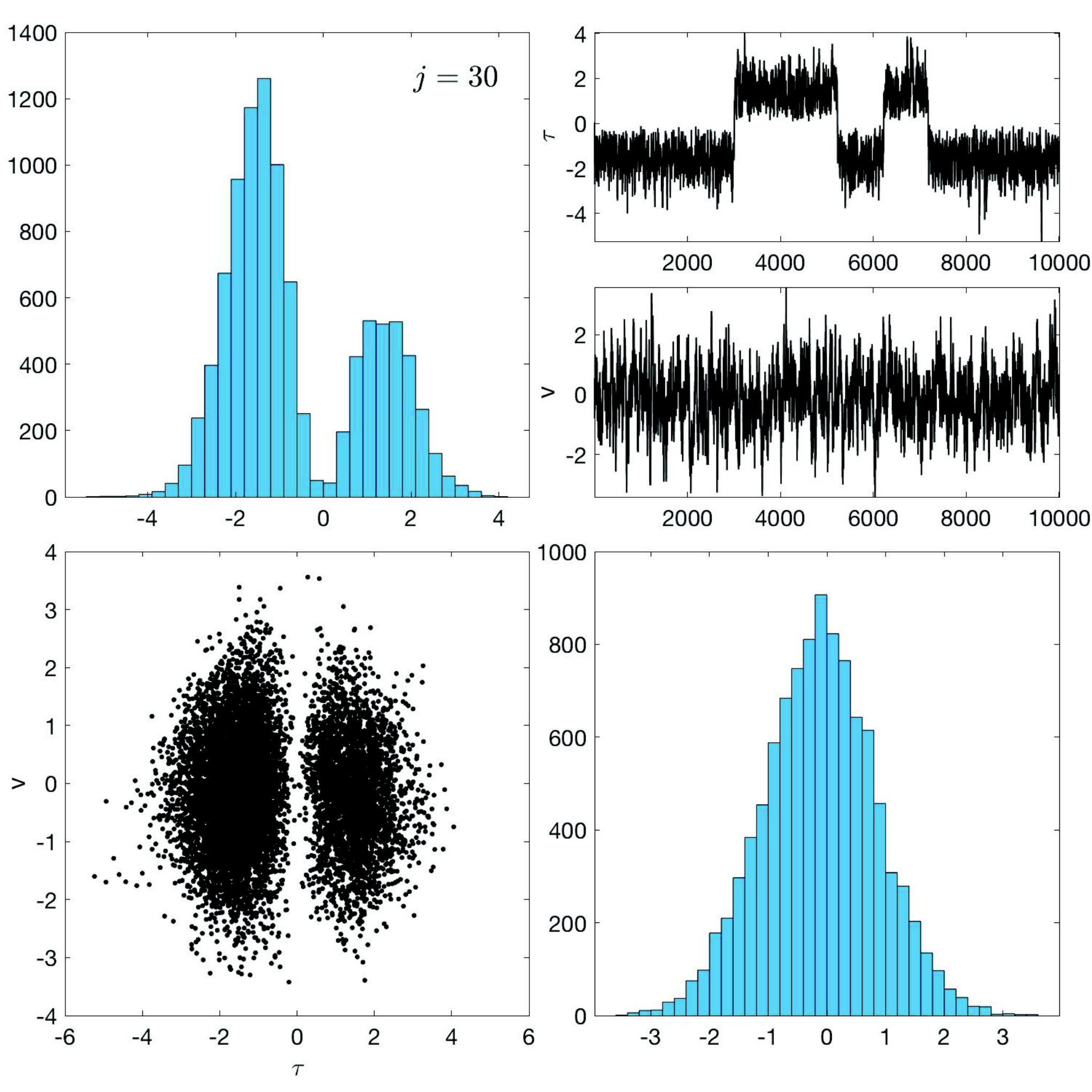
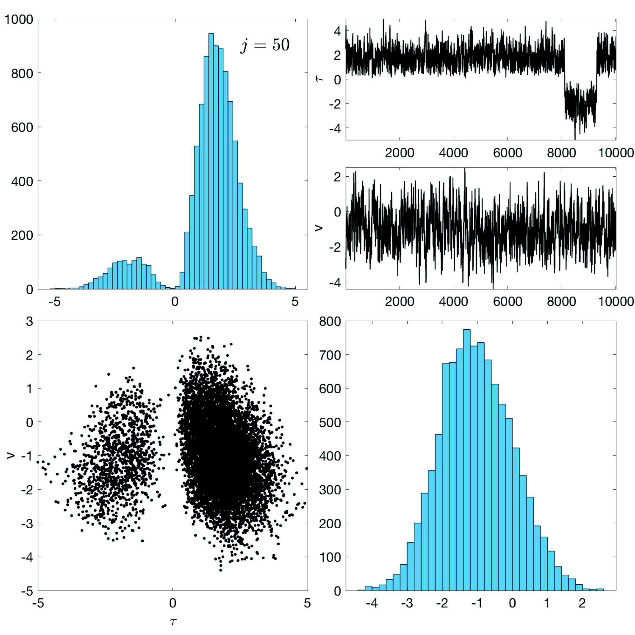
We observe that the distribution of is bimodal, reflecting the fact that the physical scaled parameter depends on which is insensitive to the sign of . Furthermore, at , the sample is centered near the coordinate origin, indicating that the sampler recognizes the point as belonging to the flat background. At , the bimodal nature is visible, however, the values of are predominantly negative, indicating a presence of a negative jump, since
However, the histogram of does not exclude the value corresponding to a background value , indicating uncertainty in identifying the jump unambiguously. Interestingly, if the stepsize is decreased to increase the acceptance rate, the sampler fails to identify the bimodal nature of the distribution and samples only from the mode . This is not a serious issue, as the bimodality is simply a result of coordinate representation, however, we chose here select the strepsize so that the feature becomes visible.
Figure 3 shows the autocorrelation functions of the retained sample of the components , and ,
where
The autocorrelation plots give a sense of the independence of the subsampled draws. There seems to be no significant difference between a background variable and one corresponding to a jump.


Before analyzing the sample further, we run similar pCN sampling using the other hypermodels. It turns out that as decreases, the sampling becomes more challenging. We start with . Using the same stepsize as in the case the acceptance rate falls to 4.8%, so we decrease the stepsize slighltly to , yielding an acceptance rate of 16.1%. Generating a sample of size 10 000 000, retaining again every 1000th sample point takes 131 seconds in a standard laptop. In this case, even with a larger stepsize, the sampler is unable to detect the coordinate bimodality and samples only from the mode where , as shown by the scatter plots in Figure 4.
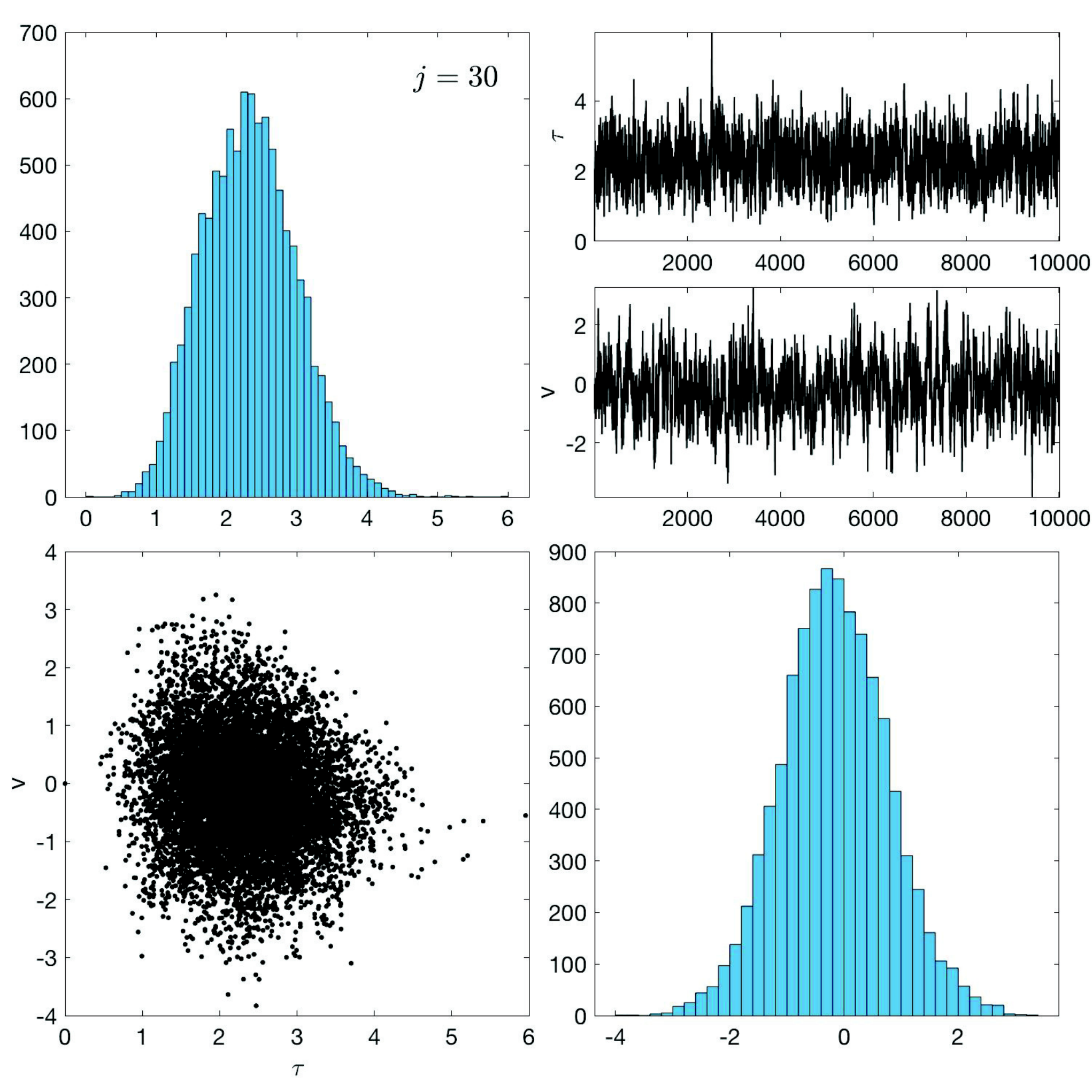
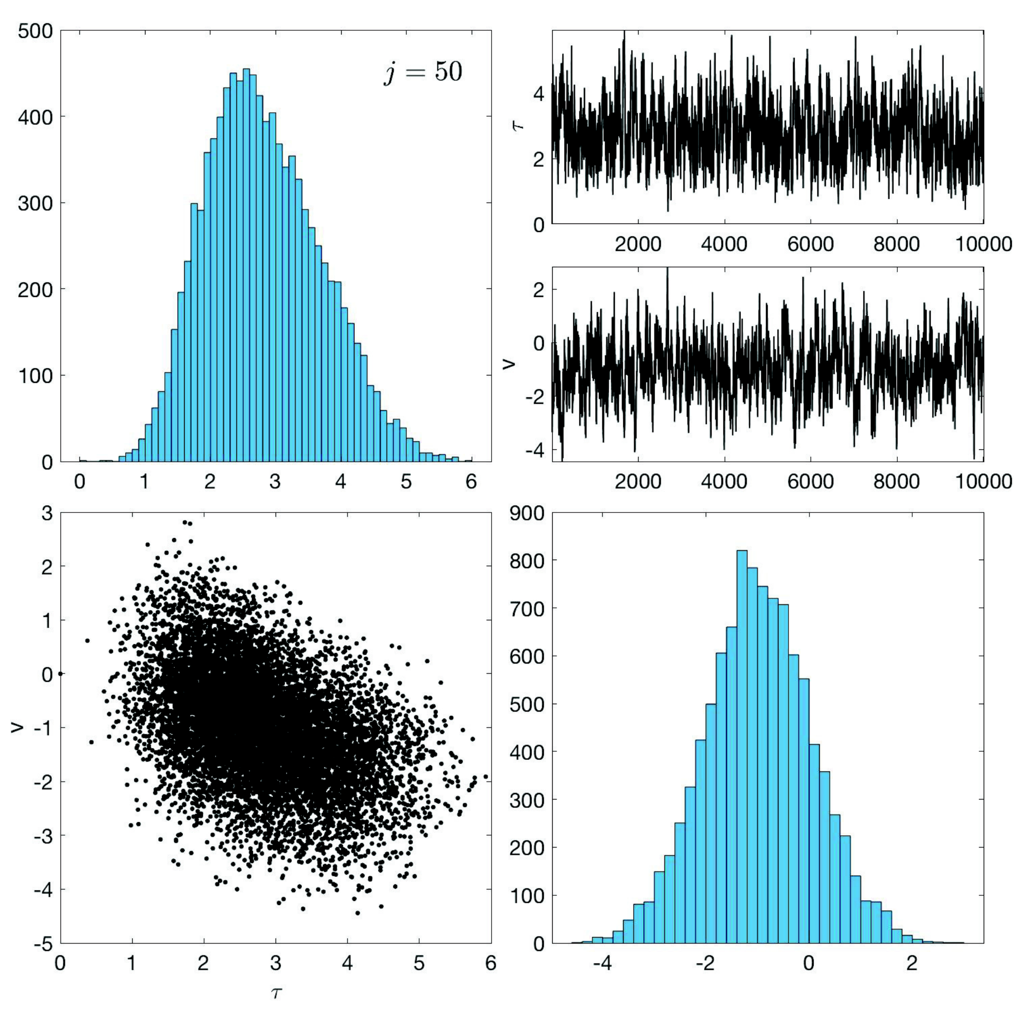
The level of independence of the draws can be inferred from the autocorrelation functions shown in Figure 3. We observe that the correlation level is not significantly different from that corresponding to the gamma hypermodel.
Consider now the hypermodels with negative , yielding a highly non-linear Gibbs energy functional with a strong sparsity promotion in the MAP estimation problems. It turns out that these models pose a challenge for sampling as well. We start with . Using the same stepsize as in the case , the acceptance rate is as low as 0.12%, so it is reasonable to decrease the stepsize. After extensive testing, we found that yields a reasonable acceptance rate of 6%, and gives a 12% acceptance. Since the former figure is close to the values in the previous experiments, we set . To make the results comparable to the previous ones, we keep the same sample size of 10 000 000, retaining every 1000th sample point. The computing times are close to the ones reported above, of the order of 110 seconds.
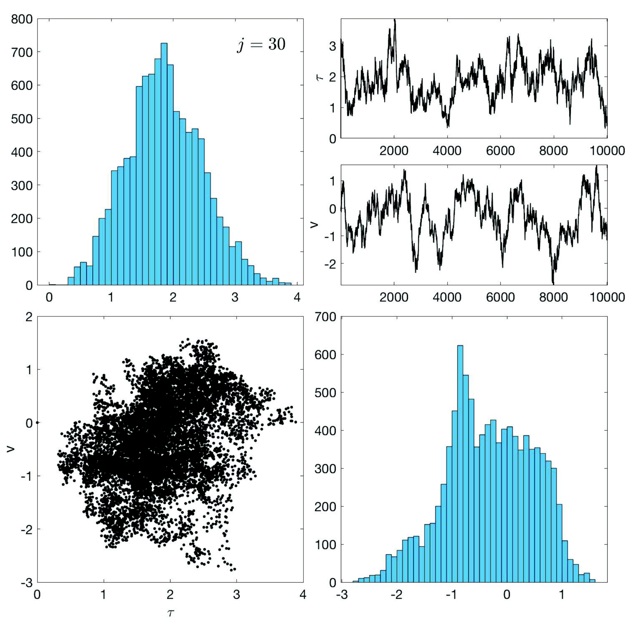
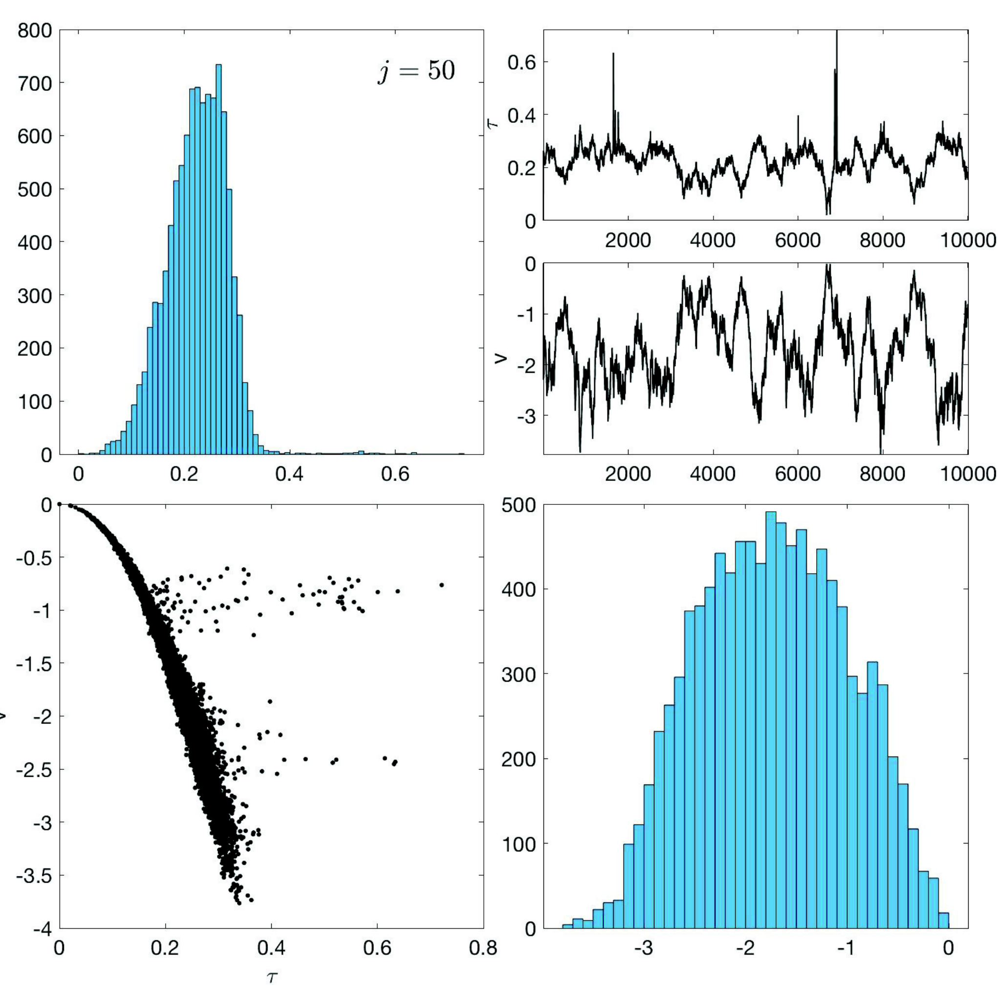
Figure 5 shows the scatter plots and histograms of the parameters . We observe that at , the points are concentrated near a parabolic curve, which is to be expected, as the variables are related to each other through the formula
and at , we expect that the likelihood favors combinations of yielding a negative value for .
The sample histories of and are not indicating a good mixing, however, from the practical point of view, the important question is how well the sample mixes the values . To explore this question, we plot again the autocorrelation functions of the selected components in Figure 6. Interestingly, while the autocorrelation functions of the -variables are decreasing rather slowly, the -variable autocorrelations indicate rather good mixing.

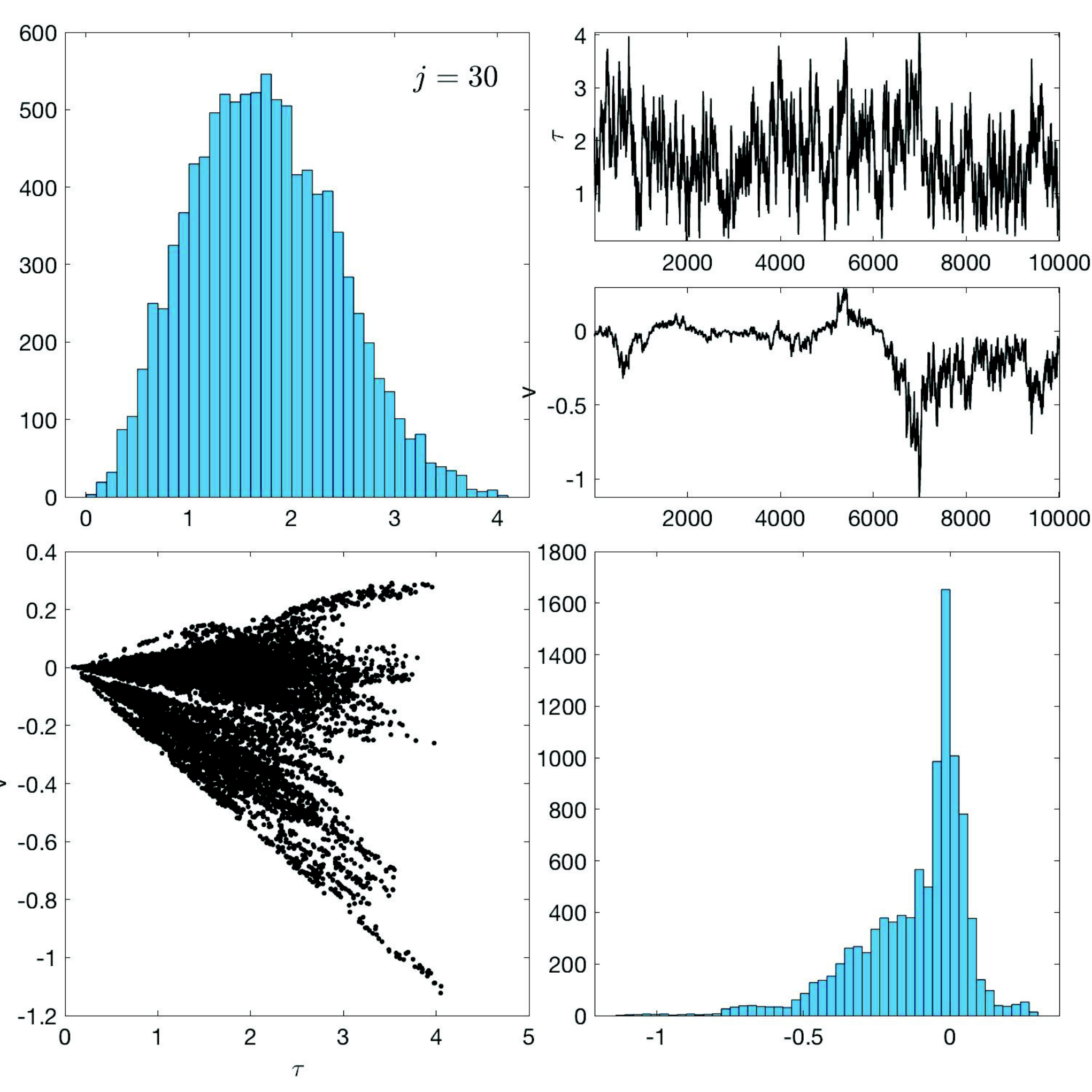
Finally, we consider the inverse gamma hyperprior, . Numerical tests indicate that the proposed sampler struggles to find a reasonably well mixed sample. To demonstrate this, we select first the step size to be , which leads to an acceptance rate as low as 0.001%, that is, one proposal of every 100 000 is accepted in the average. We then generate a sample of size , keeping only every 10 000th point, i.e., we have a sample of size 10 000 in which approximately 90% of points are repeated values corresponding to rejections. The computing time of this sample is less than 18 minutes. The scatter plots for the two selected values of are shown in Figure 7.
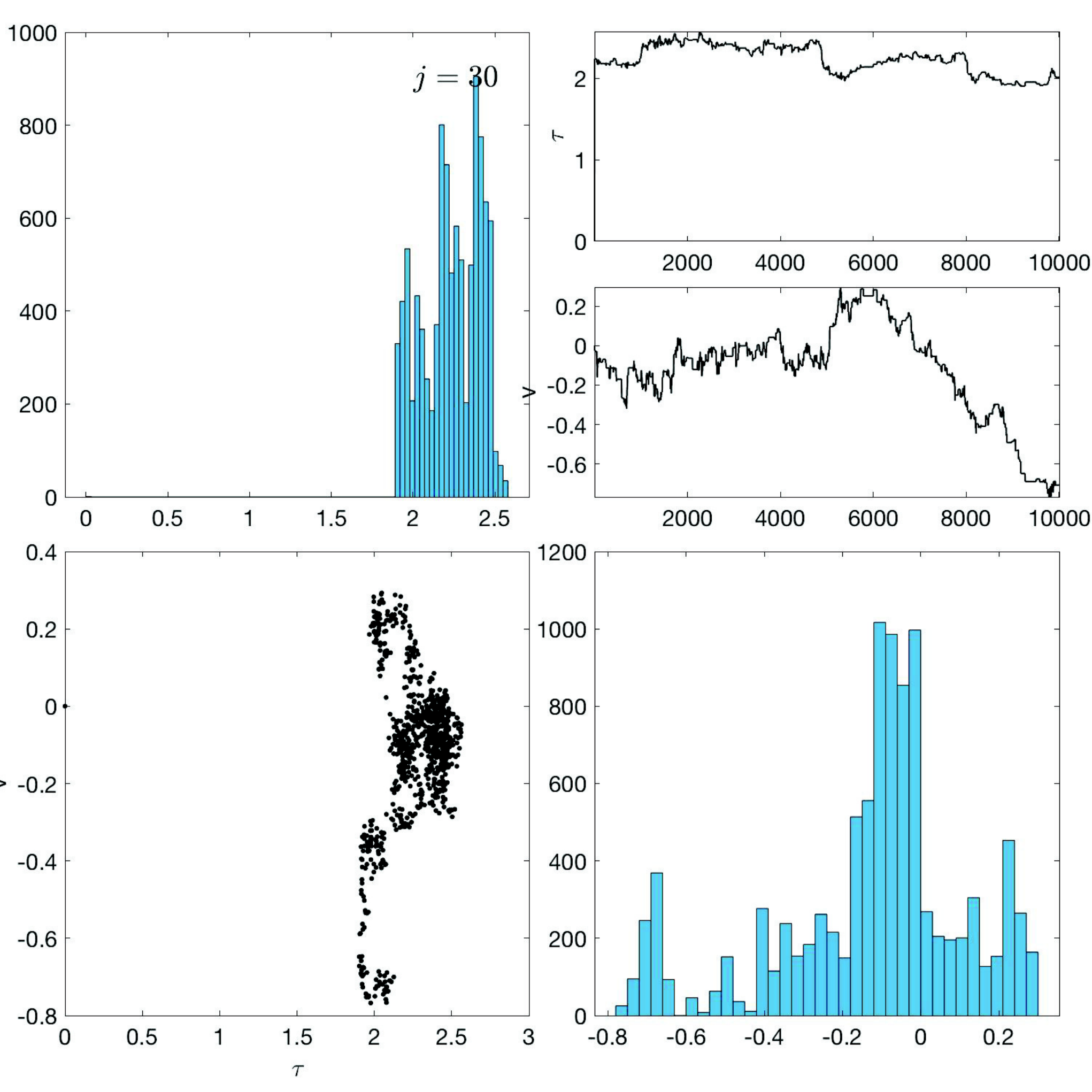
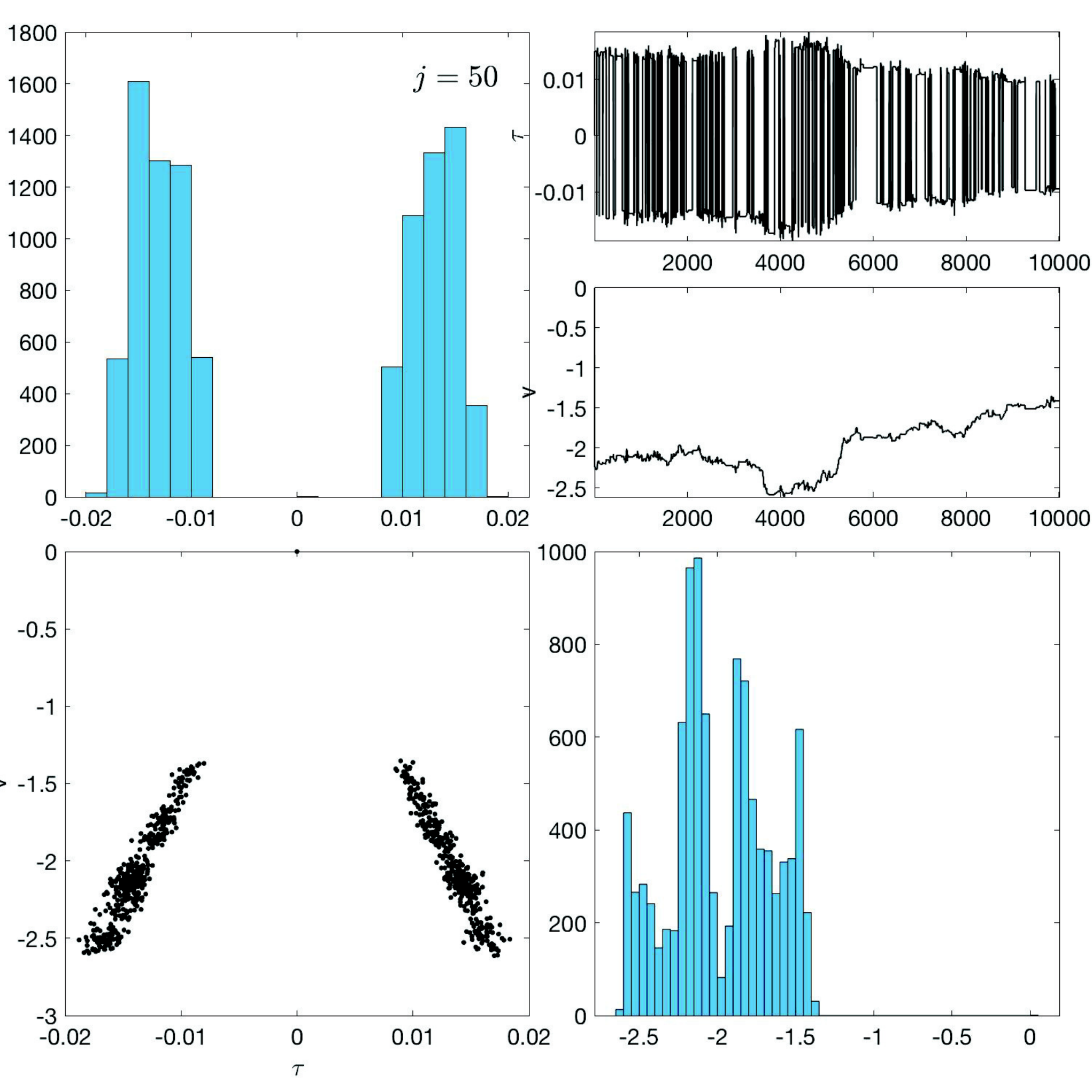
The time traces of the samples reveal that the sample is of low quality, and reliable conclusions could hardly be based on this sample. Numerical experiments show that decreasing the step size does not improve significantly the sample quality. The plots show, however, some features that may help designing a better sampler. First, the scatter plot for shows again that the coordinate transformation leads to a bimodal distribution, which is hard to reproduce with a smaller step size. Second, we observe that the sampler proposes points that lie along lines passing through the origin. Recalling that for , the coordinate transformation implies that
the absolute value of the slope of the line determines the proposed value for . It turns out that for , the sample history of is quite satisfactory, with a relatively short correlation length (not shown here.)
To improve the mixing in the case , we propose a modification of the pCN algorithm based on a reparametrization of the pairs . Consider the problem of generating a standard normal distribution in the plane . Let , and denote . We have
Let , and assume that is independent of . For any , we define
| (15) |
We claim that
This is a direct consequence of the fact that
Without loss of generality, we may assume that the coordinates are chosen so that . Then
follows a Rayleigh distribution.
Let be the phase angle of ,
For an arbitrary , define
| (16) |
Then, . Based on these observations, we introduce the following two-phase proposal:
Given , , and the current point ,
- 1.
Set , and
- 2.
Set , and
- 3.
Define
In this manner, the new variable with realization follows the same Gaussian distribution as as in the standard pCN proposal, but we control separately the stepsize in the radial and in the angular direction. The two free variables and add complexity to the tuning process, but may lead to a chain with better mixing properties.
To demonstrate the viability of the proposed algorithm, we run the sampler with parameter values and , yielding an acceptance rate of 1.5%. We compute a sample of size 5 000 000, retaining every 500th realization. The computing time is slightly longer than with plain pCN, requiring 91 seconds on a standard laptop. The scatterplots corresponding to this sample are shown in Figure 8.
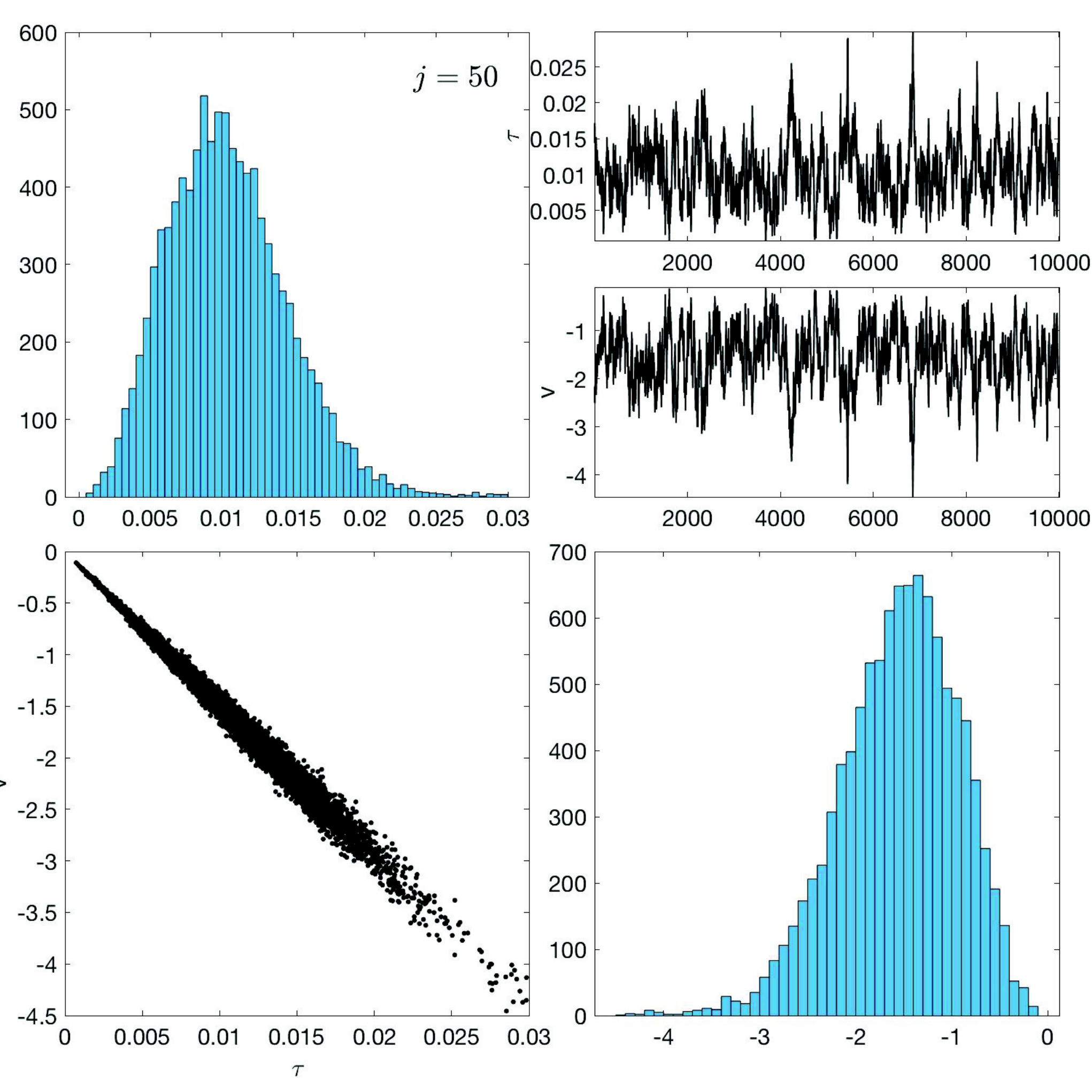
To assess the quality of the sample, we compute again the autocorrelation functions for the selected variables, see Figure 9. We observe that while the autocorrelation indicates poor quality of the sample of , the autocorrelation of decreases relatively rapidly. The conclusion therefore is that if the sample-based estimate of is small, we may claim with high certainty that is small, too.

To summarize the results of the samplers, in Figure 10 we plot the estimated posterior means and 90% credible envelopes of the variables , and corresponding to the four hypermodels.


The results show that while the MAP estimates for all models can be considered sparse solutions, the posterior means with and in particular, do not reflect the sparsity promoting nature of the prior models. This suggests that the posterior mean is not a particularly good representative summary of the posterior distribution, even if the individual samples would reflect the sparsity prior.
The smoothness of the posterior mean raises the question to what extent profiles sampled from the posterior density are compressible. To further investigate this issue, let denote the th sample vector of the variance parameter, and define -compressibility by the formula
where is a given threshold. We set the threshold to correspond to one standard deviation above the mean of the gamma distribution,
| (17) |
Figure 11 shows the histograms of the number of components in the vectors exceeding the threshold . The samples based on models and identify significantly more increments above the threshold than the cardinality of the support of the generative model, the maximum of the histograms being around twenty, while for both and , the maximum of the histogram is at 5, which coincides with the number of non-zero increments in the generative model.

5 Discussion
The difficulties of sampling from posterior densities corresponding to hierarchical Bayesian models are twofold: The curse of dimensionality makes efficient sampling hard, and the strong correlation between the parameters at different level adds an extra bottleneck for samplers. In this article, the former problem has been addressed by transforming the problem so that the preconditioned Crank-Nicholson sampling scheme can be applied. As the examples with strongly non-convex energy functionals show, the transformation does not completely remove the second problem, however, the transformation gives enough insight to allow further developments of the sampling strategy so that at least in the case of inverse gamma hyperprior model, a relatively efficient algorithm can be found. A natural question to be addressed in the future is if the proposed algorithm can be generalized or hyperprior models more general than the inverse gamma distribution.
The sampling analysis for sparsity promoting hypermodels reveals that the concept of sparsity promotion is more complex than the analysis of the maximum a posterior estimates reveals: The MAP estimate may identify the correct number of non-zero entries in a sparse vector, but sampling from the posterior density may not consistently support the level of sparsity. This was clearly demonstrated by the computed examples with parameter values and : While the MAP estimates localize well the discontinuities, the draws from the posterior seem to have significantly more discontinuities. This finding underlines also the observation that for sparse recovery, the MAP estimate may be a better summary of the posterior than the posterior mean, which in our example resembles more a smooth reconstruction than a discontinuous one.
Finally, we point out that the analysis above did not address the question of data sensitivity. It has been demonstrated that if the data have variable sensitivity to different components of the unknown, both MAP and posterior mean estimates may fail to recognize some of the non-zero components in the generative model. While the sensitivity analysis could have been included in the discussion here, it was omitted in order to keep the focus on the sampling techniques proposed in this article, but may be the topic of future work.
Acknowledgements
The work of DC was partly supported by the NSF grant DMS 1951446, and that of ES by the NSF grant DMS-2204618.
References
- [1] Agrawal, S., Kim, H., Sanz-Alonso, D. and Strang, A., 2022. A variational inference approach to inverse problems with gamma hyperpriors. SIAM/ASA Journal on Uncertainty Quantification, 10(4), pp.1533-1559.
- [2] Agapiou S, Bardsley JM, Papaspiliopoulos O and Stuart AM (2014) Analysis of the Gibbs sampler for hierarchical inverse problems. SIAM/ASA Journal on Uncertainty Quantification 2: 511-544
- [3] Aharon M, Elad M and Bruckstein A (2006) K-SVD: an algorithm for designing overcomplete dictionaries for sparse representation IEEE Trans Signal Process 54: 4311-4322
- [4] Betancourt, M. and Girolami, M., 2015. Hamiltonian Monte Carlo for hierarchical models. Current trends in Bayesian methodology with applications, 79(30), pp.2-4.
- [5] De Bortoli, V., Durmus, A., Pereyra, M. and Vidal, A.F., 2020. Maximum likelihood estimation of regularization parameters in high-dimensional inverse problems: an empirical Bayesian approach. Part II: Theoretical analysis. SIAM Journal on Imaging Sciences, 13(4), pp.1990-2028.
- [6] Calvetti D, Pascarella A, Pitolli F, Somersalo E and Vantaggi B (2019) Brain activity mapping from MEG data via a hierarchical Bayesian algorithm with automatic depth weighting. Brain topography 32: 363-393
- [7] Calvetti D, Somersalo E and Strang A (2019) Hierachical Bayesian models and sparsity: -magic. Inverse Problems 35: 035003
- [8] Calvetti D, Pragliola M, Somersalo E and Strang A (2020) Sparse reconstructions from few noisy data: analysis of hierarchical Bayesian models with generalized gamma hyperpriors. Inverse Problems 36: 025010
- [9] Calvetti D, Pragliola M and Somersalo E (2020) Sparsity promoting hybrid solvers for hierarchical Bayesian inverse problems. SIAM Journal on Scientific Computing 42: A3761-A3784
- [10] Calvetti D and Somersalo E (2008) Hypermodels in the Bayesian imaging framework. Inverse Problems 24: 034013
- [11] Calvetti D and Somersalo E (2023) Bayesian Scientific Computing. Springer Verlag, New York
- [12] Candes E and Tao T (2005) Decoding by linear programming, IEEE Trans Inf Theory 12: 4203-4215
- [13] Chen S, Donoho D and Saunders M (1998) Atomic decomposition by basis pursuit. SIAM Journal on Scientific Computing 20: 33-61
- [14] Cotter SL, Roberts GO, Stuart AM and White D (2013) MCMC methods for functions: modifying old algorithms to make them faster. Statistical Science 28: 424-446
- [15] P. Damlen, J.Wakefield, and S.Walker, Gibbs sampling for Bayesian non-conjugate and hierarchical models by using auxiliary variables, J. R. Stat. Soc. Ser. B. Stat. Methodol., 61 (1999), pp. 331-344.
- [16] Dennis JE, Schnabel R. (1996) Numerical methods for unconstrained optimization and nonlinear equations. Society for Industrial and Applied Mathematics.
- [17] Donoho DL (2006) Compressed sensing. IEEE Transactions on information theory 52: 1289-1306
- [18] Durmus, A, Moulines, É. and Pereyra, M., 2022. A Proximal Markov Chain Monte Carlo Method for Bayesian Inference in Imaging Inverse Problems: When Langevin Meets Moreau. SIAM Review, 64(4), pp.991-1028.
- [19] Glaubitz, J., Gelb, A. and Song, G., 2023. Generalized sparse Bayesian learning and application to image reconstruction. SIAM/ASA Journal on Uncertainty Quantification, 11(1), pp.262-284.
- [20] Kaipio, J.P., Kolehmainen, V., Somersalo, E. and Vauhkonen, M., 2000. Statistical inversion and Monte Carlo sampling methods in electrical impedance tomography. Inverse problems, 16(5), p.1487.
- [21] Liu J and West M (2001) Combined parameter and state estimation in simulation-based filtering. In Sequential Monte Carlo methods in practice (pp. 197-223). Springer, New York, NY
- [22] Lucka, F., 2012. Fast Markov chain Monte Carlo sampling for sparse Bayesian inference in high-dimensional inverse problems using L1-type priors. Inverse Problems, 28(12), p.125012.
- [23] S Mallat (2009) A Wavelet Tour of Signal Processing: The Sparse Way. Academic Press, third edition.
- [24] Papaspiliopoulos O, Roberts GO and Sköld M (2007) A general framework for the parametrization of hierarchical models. Statistical Science 22: 59-73
- [25] G. O. Roberts and S. K. Sahu, Updating schemes, correlation structure, blocking and parameterization for the Gibbs sampler, J. R. Stat. Soc. Ser. B. Stat. Methodol., 59 (1997), pp. 291-317.
- [26] Tibshirani R (1996) Regression shrinkage and selection via the lasso. Journal of the Royal Statistical Society, Series B 58: 267-288
- [27] Vidal, A.F., De Bortoli, V., Pereyra, M. and Durmus, A., 2020. Maximum likelihood estimation of regularization parameters in high-dimensional inverse problems: An empirical Bayesian approach part i: Methodology and experiments. SIAM Journal on Imaging Sciences, 13(4), pp.1945-1989.
- [28] Xiao, Yao, and Jan Glaubitz. ”Sequential image recovery using joint hierarchical Bayesian learning.” arXiv preprint arXiv:2206.12745 (2022).