Complete crystalline topological invariants from partial rotations in (2+1)D
invertible fermionic states and Hofstadter’s butterfly
Abstract
The theory of topological phases of matter predicts invariants protected only by crystalline symmetry, yet it has been unclear how to extract these from microscopic calculations in general. Here we show how to extract a set of many-body invariants , where o is a high symmetry point, from partial rotations in (2+1)D invertible fermionic states. Our results apply in the presence of magnetic field and Chern number , in contrast to previous work. together with , chiral central charge , and filling provide a complete many-body characterization of the topological state with symmetry group . Moreover, all these many-body invariants can be obtained from a single bulk ground state, without inserting additional defects. We perform numerical computations on the square lattice Hofstadter model. Remarkably, these match calculations from conformal and topological field theory, where -crossed modular matrices of symmetry defects play a crucial role. Our results provide additional colorings of Hofstadter’s butterfly, extending recently discovered colorings by the discrete shift and quantized charge polarization.
There has been intense work over the past decade in developing a comprehensive characterization and classification of topological phases of matter with internal Kitaev 2009; Ryu et al. 2010; Chen et al. 2013; Kapustin 2014; Kapustin et al. 2015; Wang and Gu 2020; Senthil 2015; Barkeshli et al. 2019; Barkeshli et al. 2022; Aasen et al. 2021; Bulmash and Barkeshli 2022 and crystalline symmetries Chiu et al. 2016; Cheng et al. 2016; Bradlyn et al. 2017; Po et al. 2017; Kruthoff et al. 2017; Huang et al. 2017; Thorngren and Else 2018; Cheng and Wang 2022; Zhang et al. 2022a; Elcoro et al. 2021; Manjunath and Barkeshli 2021; Manjunath and Barkeshli 2020. Despite much progress, the problem of how to fully characterize such systems, in particular by numerically extracting a complete set of invariants, remains partially solved Shiozaki et al. 2017; Shapourian et al. 2017; Zhang et al. 2022b; Zhang et al. 2023; Herzog-Arbeitman et al. 2022.
In this paper, we study (2+1)D topological states of fermions with symmetry group , which consists of charge conservation, discrete magnetic translation and point group rotation symmetries. We focus on invertible fermionic phases, which have a unique ground state on all manifolds Barkeshli et al. 2022; Aasen et al. 2021. We show how to numerically extract a set of many-body invariants associated to the crystalline symmetries by computing expectation values of partial rotations centered at high symmetry points o of the unit cell. For example, if o is preserved by rotations of order where is even, then for a fixed Chern number, and define and invariants respectively, for each o. Our numerical results are in remarkable agreement with analytical calculations from conformal and topological field theory; specifically, the invariants encode the -crossed modular matrices of symmetry defects Barkeshli et al. 2019; Manjunath and Barkeshli 2020.


For square lattice and charge conservation symmetries, the expected theoretical classification of topological invariants is given by the group Zhang et al. 2022a; Manjunath et al. 2023a. We find that the invariants , together with the Chern number , the chiral central charge and the filling , give a complete characterization of these invariants. In particular, the discrete shift and quantized charge polarization studied in Refs. Zhang et al. 2022b; Zhang et al. 2023 can be obtained from . Our methods to extract require only a single bulk ground state on a disk, without needing to insert additional defects, adding to a line of work that extracts topological invariants from single bulk ground states Levin and Wen 2006; Kitaev and Preskill 2006; Shiozaki et al. 2017; Dehghani et al. 2021; Cian et al. 2021; Cian et al. 2022; Kim et al. 2022; Fan et al. 2022.
As an application, we study the square lattice Hofstadter model and obtain a number of additional colorings of Hofstadter’s butterfly, extending the colorings by and discovered in Zhang et al. 2022b; Zhang et al. 2023. Analogous classification results hold for point group rotations of order 2,3 and 6, and will be mentioned at the end of the paper.
Partial rotations and partial translations on a cylinder have been studied in prior works and have been shown to yield invariants such as topological spins of anyons, central charges Tu et al. 2013; Zaletel et al. 2013; Kobayashi et al. 2023, and invariants of symmetry-protected topological (SPT) states Zaletel 2014; Shiozaki et al. 2017; Shiozaki et al. 2018; Kobayashi and Shiozaki 2019; You et al. 2020. In contrast our results apply both in the presence of arbitrary rational magnetic flux, , demonstrate a complete set of invariants for crystalline symmetries, and also incorporate several subtleties missed in prior work. These include the proper use of -crossed modular matrices, the quantization of , and their dependence on o.
Symmetries and model.
We study gapped phases of matter with the symmetry group , where denotes magnetic lattice translations, for denotes point group rotations. We assume throughout, and briefly comment on at the end of the paper.
The symbol implies that the magnetic translation operators, generated by , obey the algebra where is the total fermion number. The tilde indicates that the definition of the operator involves a gauge transformation. Note , which is fermion parity.
Let be the smallest angle of rotation which preserves the rotation center o. The possible high symmetry points o of the square lattice are shown in Fig. 2; they are (plaquette center and vertex respectively, with ) and (edge center, with ) 11 1 Note we will abuse language somewhat and use o both as the rotation center and as a maximal Wyckoff position.. As shown in Zhang et al. 2022b; Zhang et al. 2023 and reviewed in App. A, there is a canonical choice of magnetic point group rotation operators which are centered at o and satisfy . We also define another set of operators , and . Note that and .
We study the spinless free fermion Hofstadter model with flux per unit cell, with Hamiltonian . Our numerical methods and theoretical analysis hold even if we consider further neighbor hopping and/or interaction terms.

Partial rotation calculation. Consider a state , which can be defined on a system with either open or periodic boundary conditions. Let be the restriction of to an invariant subregion centered at o.
We find that . sets the real-valued amplitude. When is an integer, we find
| (1) |
is the discrete shift, which was studied in Refs.Zhang et al. 2022b; Zhang et al. 2023 and was referred to there as . Here we define analogously, as the term linear in in Eq. 1. Empirically we observe that may not be invariant throughout a given lobe in the Hofstadter model: can jump by multiples of within a single lobe, but there are no jumps in . For an intuitive explanation of these jumps, which are system size dependent, see App. A. We thus define
| (2) |
The main result of this paper is that are topological invariants protected by point group rotational symmetry about o. is in general an integer or half-integer, while is a multiple of . For a fixed Chern number, they can take and different values respectively and thus define and invariants, respectively. We find both empirically and analytically using Eq. 10 that , and so it will henceforth be ignored. When , are closely related to the many-body real-space indicators defined in Herzog-Arbeitman et al. 2022.
The values of are plotted for the square lattice Hofstadter model in Figs. 1, 2, and 3. The values of satisfy the empirical relation
| (3) |
where is an integer. The subscript 3 is used to match a convention from Manjunath and Barkeshli 2021. satisfies
| (4) |
where and is an integer. Eqs. (3), (4) are in excellent agreement with a conformal field theory calculation, which predicts the basic quantization and dependence of exactly, but does not give the actual values of and for a particular model. The CFT prediction is summarized by Eq. (10).
If we view in the square lattice Hofstadter model as a function of , has period while has period . A similar periodicity depending on origin was observed for the discrete shift in Ref. Zhang et al. 2023. Mathematically, the lack of periodicity in arises because is not a gauge-invariant operator, and is only periodic (without a gauge transformation) under (For details see App. A). The lack of periodicity is physically meaningful and arises because must be defined as a real number to consistently specify generic perturbations of Zhang et al. 2023.
The continuum limit of the Hofstadter model is obtained by taking . In this limit states with Chern number are equivalent to filled Landau levels (LLs), and we have
| (5) | ||||
| (6) |
As explained below, we can derive Eqs. 5, 6 analytically using results from CFT and TQFT, and also verify them empirically in our numerical calculations. are closely related to the topological term which appears in the effective response theory of continuum LLs coupled to an spin connection Wen and Zee 1992.
The empirical data for can be fit to precise formulas throughout the square lattice Hofstadter model, which we use to fully color the butterflies in Fig. 1,2. These equations all have the general form
| (7) |
Eq. (7) indicates that we can express any given state with as a stack of filled LLs (which contribute ) and a state with zero Chern number (which contributes ). Thus, specifies how the given state differs from the limit of filled LLs. The empirical formulas for throughout the butterfly are summarized in App. A. We have not obtained empirical formulas for as these are substantially more complicated.
Verification using conformal field theory.
Eqs. (3), (4) can be analytically derived by using the cut-and-glue approach established in Qi et al. 2012, which describes the entanglement spectrum of the disk subregion in the long wavelength limit by that of the (1+1)D CFT on its edge. That is, the reduced density matrix for the disk subregion is effectively given by , where denotes the CFT on the edge of the disk. The edge of the disk entangled with the complement subsystem is described by a thermal density matrix of a perturbed edge CFT within a fixed topological sector Li and Haldane 2008. The form of the perturbation in the entanglement Hamiltonian is not universal. In the following, we assume that the entanglement Hamiltonian is that of the unperturbed CFT: , and check the validity of this assumption with our numerics.
In accordance with the crystalline equivalence principle Thorngren and Else 2018; Manjunath et al. 2023b, the rotation symmetry acts as a translation symmetry combined with an internal symmetry of the CFT on the boundary of . The expectation value of for the disk without any additional flux insertion is hence evaluated in terms of the symmetry generators in the CFT as follows:
| (8) |
where we introduced the velocity of the CFT, finite temperature correlation length of the edge theory , the length of the boundary , and denotes the boundary condition with respect to fermion parity symmetry. The action of the -fold rotation on the CFT is expressed as the combination , where generates an internal (resp. ) symmetry when we take the rotation symmetry to be (resp. ). is the normalized translation operator
| (9) |
so that on the vacuum state of the CFT. with , is the CFT character that corresponds to the partition function on a torus equipped with spin structure and gauge field. As shown in App. C, the above CFT characters at high temperature can be evaluated using the modular matrices of the -crossed braided fusion category Barkeshli et al. 2019; Manjunath and Barkeshli 2020 describing the invertible phase. Our calculation uses the precise defect sectors of the -crossed modular matrices that correspond to the boundary conditions which define the CFT character; the use of -crossed modularity allows us to readily treat any symmetry action on the state encoded in the classification of fermionic invertible phases in (2+1)D Barkeshli et al. 2022; Aasen et al. 2021, some of whose details are missed in Ref. Shiozaki et al. 2017. The results for even are to leading order given by
| (10) |
where
| (11) |
for integers and . Eqs. (10) and (11) directly give Eqs. (3), (4). Moreover, we have an equivalence which comes from relabelling symmetry defects in the CFT by fermions, but no such equivalence for . We set to describe the non-interacting Hofstadter model. Combining Eqs. (10) and (11) gives
| (12) |
Relation to topological action.
appear in a general topological action which was derived for (2+1)D bosonic topological phases with symmetry in Refs. Manjunath and Barkeshli 2021; Manjunath and Barkeshli 2020, and extended to invertible fermionic systems in the appendix of Ref. Zhang et al. 2022b. It is written in terms of a gauge field , and crystalline gauge fields . is a background ‘rotation’ gauge field, which is treated as a real field with quantized holonomies. We can define as a gauge field or a gauge field corresponding to the subgroups of generated by and respectively. We use and superscripts for the coefficients that appear in the action in each case. The coefficients with supercript can be obtained by replacing in the action with only superscripts.
The full action includes a term , where is quantized mod , while is a contribution from the framing anomaly Witten 1989; Gromov et al. 2015. The quantities determine the invariant of invertible phases protected purely by rotations about o Cheng and Wang 2022, and arise in the CFT computation above through the -crossed modular matrices. are directly related to , by Eq. (12). We defer a discussion of the remaining topological response coefficients, which include an angular momentum polarization and angular momentum filling , to Ref. Manjunath et al. 2023a.
For continuum Landau levels, is an origin- independent invariant associated to continuous rotational symmetry. Now is the coefficient of the term that arises in the effective action upon integrating out the fermion fields Wen and Zee 1992, , where is the spin of the fermion in the th LL; and is similarly obtained after replacing . Moreover, in the continuum limit of the Hofstadter model, we have . After simplification (see App. D), we obtain
| (13) |
Combining Eq. (Relation to topological action.) and Eq. (12) provides the analytical derivation of Eqs. (5) and (6).
Classification.
There are various relationships involving :
| (14) | ||||
| (15) |
Eqs. (14), (15) can be derived in the LL limit (where but ) using Eq. (5), (6) and in the case of using a real-space Wannier function argument Manjunath et al. 2023a; combining the two results using linearity under stacking gives (14), (15). Eq. (15) implies that the 5 invariants define 4 independent invariants.
Eqs. (3), (4) imply that , , and are integers modulo , , and , respectively. Additionally, is an integer modulo . This can also be established in the LL limit using (5), (6) and in the case of using a real-space Wannier function argument, and finally by combining the two using linearity under stacking.
The above results imply that . But note that the overall classification of invertible fermionic phases with is a group Zhang et al. 2022a; Manjunath et al. 2023a. The three invariants are , , . A subset of this classification which assumes was derived in Ref. Zhang et al. 2022a through a real space construction. The full derivation will be explained in detail in a forthcoming work Manjunath et al. 2023a, which also shows that are independent. From this, we can conclude that , or equivalently fully characterize invertible fermionic states with symmetry group .
Discussion.
We have obtained the remarkable result that we can extract a complete set of invariants (apart from ) from partial rotations, without inserting any extra magnetic flux or lattice defects. As a corollary, we can extract the previously studied invariants in terms of as well, using Eq. (14) and the relationships between and derived in Zhang et al. 2023. We also showed how to understand the topological response theory coefficients in terms of .
We can instead study the eigenvalues of a global rotation operator on a torus; this was used in Zhang et al. 2022b; Zhang et al. 2023 to find , and also discussed in Ref. Herzog-Arbeitman et al. 2022. Some preliminary results for global rotations are shown in App. B; it is unclear how much of the classification can be obtained in this way.
It is worth highlighting that we have extracted from a single wave function without requiring the insertion of additional magnetic flux or lattice defects. Note that one can also extract from a single wave function the quantities Li and Haldane 2008; Zaletel et al. 2013; Tu et al. 2013; Kim et al. 2022, Shiozaki et al. 2017; Dehghani et al. 2021; Cian et al. 2021; Fan et al. 2022, and . The above discussion then implies that one can in principle extract all the many-body invariants characterizing an invertible state with from a single wavefunction.
Above, we focused on the square lattice, with and or 4. For any orientation preserving space group symmetry, we have the following results Manjunath et al. 2023a. If , defines a invariant, while defines a invariant. (This means that if we know , and can take and values respectively, although their precise quantization will depend on .) On the other hand, if , both and define invariants. In either case, along with and , fully characterize the many-body crystalline invariants of systems with symmetry , and these can be extracted using a single wave function.
Acknowledgements.
This work is supported by NSF CAREER grant (DMR- 1753240), and the Laboratory for Physical Sciences through the Condensed Matter Theory Center. RK is supported by a JQI postdoctoral fellowship at the University of Maryland.
References
- Kitaev (2009) A. Kitaev, Periodic table for topological insulators and superconductors, AIP Conference Proceedings 1134, 22 (2009), https://aip.scitation.org/doi/pdf/10.1063/1.3149495 .
- Ryu et al. (2010) S. Ryu, A. P. Schnyder, A. Furusaki, and A. W. W. Ludwig, Topological insulators and superconductors: tenfold way and dimensional hierarchy, New J. Phys. 12, 065010 (2010).
- Chen et al. (2013) X. Chen, Z.-C. Gu, Z.-X. Liu, and X.-G. Wen, Symmetry protected topological orders and the group cohomology of their symmetry group, Phys. Rev. B 87, 155114 (2013).
- Kapustin (2014) A. Kapustin, Symmetry protected topological phases, anomalies, and cobordisms: beyond group cohomology, arXiv preprint arXiv:1403.1467 (2014).
- Kapustin et al. (2015) A. Kapustin, R. Thorngren, A. Turzillo, and Z. Wang, Fermionic symmetry protected topological phases and cobordisms, Journal of High Energy Physics 2015, 1 (2015).
- Wang and Gu (2020) Q.-R. Wang and Z.-C. Gu, Construction and classification of symmetry-protected topological phases in interacting fermion systems, Phys. Rev. X 10, 031055 (2020).
- Senthil (2015) T. Senthil, Symmetry Protected Topological phases of Quantum Matter, Ann. Rev. Condensed Matter Phys. 6, 299 (2015), arXiv:1405.4015 [cond-mat.str-el] .
- Barkeshli et al. (2019) M. Barkeshli, P. Bonderson, M. Cheng, and Z. Wang, Symmetry fractionalization, defects, and gauging of topological phases, Phys. Rev. B 100, 115147 (2019), arXiv:1410.4540 .
- Barkeshli et al. (2022) M. Barkeshli, Y.-A. Chen, P.-S. Hsin, and N. Manjunath, Classification of d invertible fermionic topological phases with symmetry, Phys. Rev. B 105, 235143 (2022).
- Aasen et al. (2021) D. Aasen, P. Bonderson, and C. Knapp, Characterization and classification of fermionic symmetry enriched topological phases (2021), arXiv:2109.10911 [cond-mat.str-el] .
- Bulmash and Barkeshli (2022) D. Bulmash and M. Barkeshli, Fermionic symmetry fractionalization in dimensions, Phys. Rev. B 105, 125114 (2022).
- Chiu et al. (2016) C.-K. Chiu, J. C. Y. Teo, A. P. Schnyder, and S. Ryu, Classification of topological quantum matter with symmetries, Rev. Mod. Phys. 88, 035005 (2016).
- Cheng et al. (2016) M. Cheng, M. Zaletel, M. Barkeshli, A. Vishwanath, and P. Bonderson, Translational symmetry and microscopic constraints on symmetry-enriched topological phases: A view from the surface, Phys. Rev. X 6, 041068 (2016).
- Bradlyn et al. (2017) B. Bradlyn, L. Elcoro, and e. a. Jennifer Cano, Topological quantum chemistry, Nature 547, 298 (2017).
- Po et al. (2017) H. C. Po, A. Vishwanath, and H. Watanabe, Symmetry-based indicators of band topology in the 230 space groups, Nature Communications 8, 10.1038/s41467-017-00133-2 (2017).
- Kruthoff et al. (2017) J. Kruthoff, J. de Boer, J. van Wezel, C. L. Kane, and R.-J. Slager, Topological classification of crystalline insulators through band structure combinatorics, Phys. Rev. X 7, 041069 (2017).
- Huang et al. (2017) S.-J. Huang, H. Song, Y.-P. Huang, and M. Hermele, Building crystalline topological phases from lower-dimensional states, Phys. Rev. B 96, 205106 (2017).
- Thorngren and Else (2018) R. Thorngren and D. V. Else, Gauging spatial symmetries and the classification of topological crystalline phases, Phys. Rev. X 8, 011040 (2018).
- Cheng and Wang (2022) M. Cheng and C. Wang, Rotation symmetry-protected topological phases of fermions, Phys. Rev. B 105, 195154 (2022).
- Zhang et al. (2022a) J.-H. Zhang, S. Yang, Y. Qi, and Z.-C. Gu, Real-space construction of crystalline topological superconductors and insulators in 2d interacting fermionic systems, Phys. Rev. Res. 4, 033081 (2022a).
- Elcoro et al. (2021) L. Elcoro, B. Wieder, Z. Song, Y. Xu, B. Bradlyn, and B. A. Bernevig, Magnetic topological quantum chemistry, Nature Communications 12, https://doi.org/10.1038/s41467-021-26241-8 (2021).
- Manjunath and Barkeshli (2021) N. Manjunath and M. Barkeshli, Crystalline gauge fields and quantized discrete geometric response for abelian topological phases with lattice symmetry, Phys. Rev. Research 3, 013040 (2021).
- Manjunath and Barkeshli (2020) N. Manjunath and M. Barkeshli, Classification of fractional quantum hall states with spatial symmetries (2020), arXiv:2012.11603 [cond-mat.str-el] .
- Shiozaki et al. (2017) K. Shiozaki, H. Shapourian, and S. Ryu, Many-body topological invariants in fermionic symmetry-protected topological phases: Cases of point group symmetries, Phys. Rev. B 95, 205139 (2017).
- Shapourian et al. (2017) H. Shapourian, K. Shiozaki, and S. Ryu, Many-body topological invariants for fermionic symmetry-protected topological phases, Phys. Rev. Lett. 118, 216402 (2017).
- Zhang et al. (2022b) Y. Zhang, N. Manjunath, G. Nambiar, and M. Barkeshli, Fractional disclination charge and discrete shift in the hofstadter butterfly, Phys. Rev. Lett. 129, 275301 (2022b).
- Zhang et al. (2023) Y. Zhang, N. Manjunath, G. Nambiar, and M. Barkeshli, Quantized charge polarization as a many-body invariant in crystalline topological states and hofstadter butterflies, Phys. Rev. X 13, 031005 (2023).
- Herzog-Arbeitman et al. (2022) J. Herzog-Arbeitman, B. A. Bernevig, and Z.-D. Song, Interacting topological quantum chemistry in 2d: Many-body real space invariants (2022), arXiv:2212.00030 [cond-mat.str-el] .
- Manjunath et al. (2023a) N. Manjunath, V. Calvera, and M. Barkeshli, to appear (2023a).
- Levin and Wen (2006) M. Levin and X.-G. Wen, Detecting topological order in a ground state wave function, Phys. Rev. Lett. 96, 110405 (2006).
- Kitaev and Preskill (2006) A. Kitaev and J. Preskill, Topological entanglement entropy, Physical review letters 96, 110404 (2006).
- Dehghani et al. (2021) H. Dehghani, Z.-P. Cian, M. Hafezi, and M. Barkeshli, Extraction of the many-body chern number from a single wave function, Physical Review B 103, 075102 (2021).
- Cian et al. (2021) Z.-P. Cian, H. Dehghani, A. Elben, B. Vermersch, G. Zhu, M. Barkeshli, P. Zoller, and M. Hafezi, Many-body chern number from statistical correlations of randomized measurements, Physical Review Letters 126, 050501 (2021).
- Cian et al. (2022) Z.-P. Cian, M. Hafezi, and M. Barkeshli, Extracting wilson loop operators and fractional statistics from a single bulk ground state (2022), arXiv:2209.14302 [cond-mat.str-el] .
- Kim et al. (2022) I. H. Kim, B. Shi, K. Kato, and V. V. Albert, Chiral central charge from a single bulk wave function, Phys. Rev. Lett. 128, 176402 (2022).
- Fan et al. (2022) R. Fan, R. Sahay, and A. Vishwanath, Extracting the quantum hall conductance from a single bulk wavefunction (2022), arXiv:2208.11710 .
- Tu et al. (2013) H.-H. Tu, Y. Zhang, and X.-L. Qi, Momentum polarization: An entanglement measure of topological spin and chiral central charge, Physical Review B 88, 10.1103/physrevb.88.195412 (2013), arXiv:1212.6951 .
- Zaletel et al. (2013) M. P. Zaletel, R. S. K. Mong, and F. Pollmann, Topological characterization of fractional quantum hall ground states from microscopic hamiltonians, Phys. Rev. Lett. 110, 236801 (2013).
- Kobayashi et al. (2023) R. Kobayashi, T. Wang, T. Soejima, R. S. K. Mong, and S. Ryu, Extracting higher central charge from a single wave function (2023), arXiv:2303.04822 [cond-mat.str-el] .
- Zaletel (2014) M. P. Zaletel, Detecting two-dimensional symmetry-protected topological order in a ground-state wave function, Physical Review B 90, 10.1103/physrevb.90.235113 (2014).
- Shiozaki et al. (2018) K. Shiozaki, H. Shapourian, K. Gomi, and S. Ryu, Many-body topological invariants for fermionic short-range entangled topological phases protected by antiunitary symmetries, Physical Review B 98, 10.1103/physrevb.98.035151 (2018).
- Kobayashi and Shiozaki (2019) R. Kobayashi and K. Shiozaki, Anomaly indicator of rotation symmetry in (3+1)d topological order (2019), arXiv:1901.06195 .
- You et al. (2020) Y. You, J. Bibo, and F. Pollmann, Higher-order entanglement and many-body invariants for higher-order topological phases, Phys. Rev. Research 2, 033192 (2020).
- (44) Note we will abuse language somewhat and use o both as the rotation center and as a maximal Wyckoff position.
- Wen and Zee (1992) X. G. Wen and A. Zee, Shift and spin vector: New topological quantum numbers for the hall fluids, Phys. Rev. Lett. 69, 953 (1992).
- Qi et al. (2012) X.-L. Qi, H. Katsura, and A. W. W. Ludwig, General relationship between the entanglement spectrum and the edge state spectrum of topological quantum states, Physical Review Letters 108, 10.1103/physrevlett.108.196402 (2012), arXiv:1103.5437 [cond-mat.mes-hall] .
- Li and Haldane (2008) H. Li and F. D. M. Haldane, Entanglement spectrum as a generalization of entanglement entropy: Identification of topological order in non-abelian fractional quantum hall effect states, Phys. Rev. Lett. 101, 010504 (2008).
- Manjunath et al. (2023b) N. Manjunath, V. Calvera, and M. Barkeshli, Nonperturbative constraints from symmetry and chirality on majorana zero modes and defect quantum numbers in (2+1) dimensions, Phys. Rev. B 107, 165126 (2023b).
- Witten (1989) E. Witten, Quantum field theory and the Jones polynomial, Comm. Math. Phys. 121, 351 (1989).
- Gromov et al. (2015) A. Gromov, G. Y. Cho, Y. You, A. G. Abanov, and E. Fradkin, Framing anomaly in the effective theory of the fractional quantum hall effect, Phys. Rev. Lett. 114, 016805 (2015).
Appendix A Further details on the numerics
A.1 Definition of vector potential
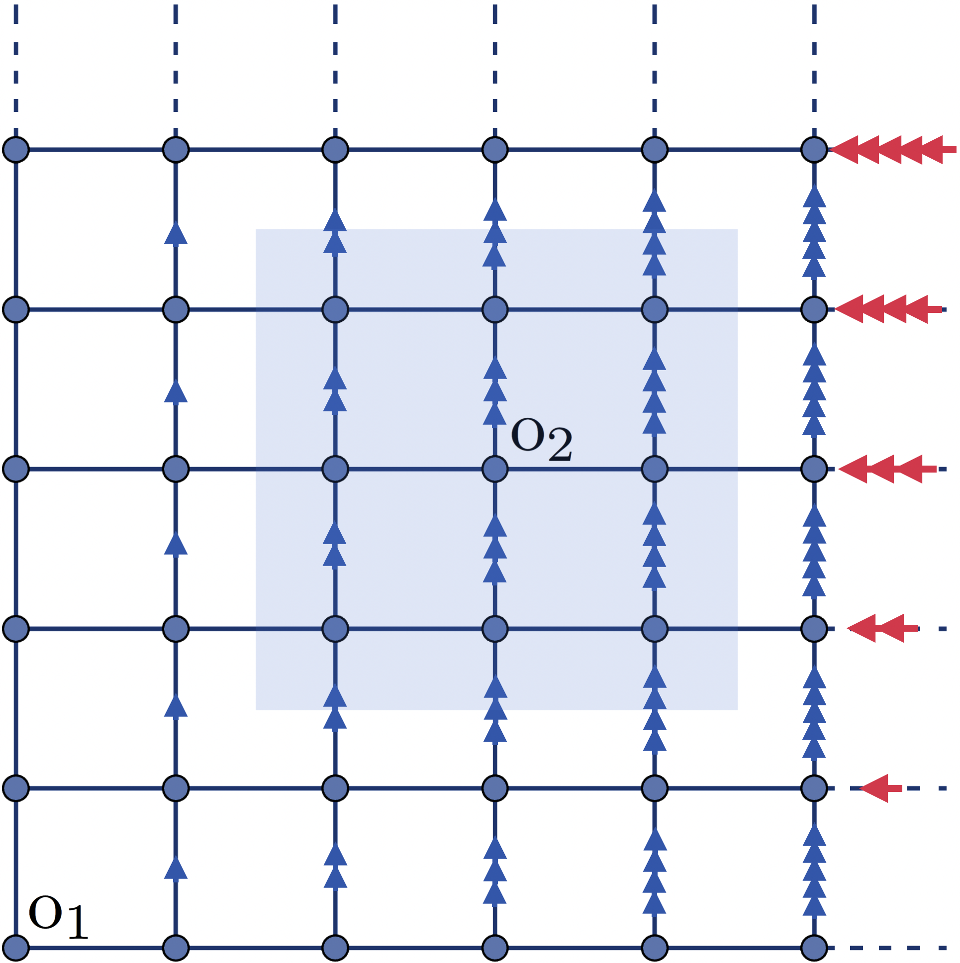
In this section we provide a definition of the vector potential for the square lattice Hofstadter model on a torus. Some of the following details have previously appeared in Ref. Zhang et al. 2022b. We first define our vector potential on a torus with even. Considering even is sufficient for our calculations on the torus. An example of the gauge choice is shown in Fig. 4. We can use a similar gauge to define on an open disc.
A.2 Choice of global rotation operator
In systems with and point group rotation symmetries, we have the ambiguity that any rotation symmetry operator can be multiplied by a phase to give another valid symmetry operator. It is necessary to fix this ambiguity in order to uniquely define a rotation operator. Below we illustrate how to do this on the infinite plane, and then on the torus.
A.2.1 On the infinite plane
Ref. Zhang et al. 2022b showed how to canonically define one such operator ( in the notation of this paper) on the infinite plane, which assigns zero excess flux around a disclination of angle created at o using . Since the defect Hamiltonian depends on the specific choice of gauge transformation defining , considering a different operator modifies the flux around the disclination by , and therefore we can physically distinguish it from . See Ref. Zhang et al. 2022b for the explicit construction of a disclination Hamiltonian with fourfold rotational symmetry.
Let us specialize to the case and . Assume each plaquette on the infinite plane has flux . If (a vertex), the four possible operators assign equal flux to all plaquettes in the lattice with a disclination, except one that lies next to the disclination. In this plaquette the assigned flux is , where . Thus there is a canonical choice of , corresponding to (meaning zero excess flux). When (a plaquette center), there is a triangular plaquette at a disclination which is assigned a flux . The operator for which is also canonical, because it assigns a flux at the disclination that is proportional to .
To extract the desired topological invariants in this paper, it turns out to be insufficient to use the operators alone, because they only generate groups of order . Thus we also define , which is of order and satisfies . The two sets of operators, together denoted , are indeed sufficient for our purpose. Arbitrary rotations can be considered by defining . Note that insert excess flux at a disclination, compared to and respectively.
A.2.2 On the torus
Defining a unique rotation operator on a torus with fourfold rotational symmetry is slightly more subtle than on the infinite plane, because any order 4 rotation preserves 2 points . If the side length of the torus is even, the two fixed points are either both at or both at . If is odd, we have one fixed point each at and .
can be defined for or by restricting to a disc centered around o, and creating a disclination within centered at o, using . As in the case of the infinite plane discussed above, we canonically define such that creates a disclination with zero excess flux. We then define and .
A.3 Partial rotation on a torus
Given the global rotation operators , we wish to restrict them to a region , hence obtaining . Note that the chosen operator inserts excess flux in a disclination centered at o relative to . We find that the result for follows Eq. (1).
A.4 Partial rotation on an open disc
We can also perform the partial rotation calculation on an open disc. This can be done by first defining the vector potential similarly as in Fig. 4, using a gauge which inserts flux per plaquette in some region. As shown in Fig. 5, It is not necessary that the vector potential has support on the whole disc: the flux needs to be inserted only in an invariant subregion around o. Besides, does not have to be defined around the center of the subregion with flux, as long as is enclosed by this subregion. The center of , which we define as o, can be at any maximal Wyckoff point.
On the torus, we have a global rotation symmetry operator , and we define to be the restriction of to region . On the disc, this cannot be done as there might not be a global symmetry operator to start with. Therefore, we first choose and then define an operator , which commutes with the Hamiltonian restricted to . We find that choosing linear size of to be too large () or too small () gives unquantized , which is tested this for . As before, we need to impose a constraint on to fix the ambiguity by a global phase . This can be done by fixing the excess flux inserted around a disclination created using the operator as explained in the previous section. We define (respectively ) so that it inserts an excess flux of at a disclination, relative to .
Note that, we obtain the same result, Eq. (1), on the torus or the open disc, as long as we choose o at the same maximal Wyckoff position, and choose a partial rotation operator that inserts the same flux around a disclination at o.

A.5 Details on the jumps of

As stated in the main text, if we use the operators , sometimes jumps by inside a single Hofstadter lobe, as seen in Fig. 6. We define in order to eliminate these jumps. In general, the position of these jumps will depend on the system size and the size of the partial rotation region, but the value of these jumps is always . We can understand these jumps as follows. The following arguments are equivalent to those given in Herzog-Arbeitman et al. 2022 using the many-body real space invariants defined there.
Suppose in a system where all orbitals are filled (). First consider . Let be the value of at . Now suppose we minimally enlarge the partial rotation region by enclosing more sites which rotate into each other Under . The states at these 4 sites form an orbit of size 4 under and contribute extra phases of , which are fourth roots of 1. The expectation value of will gain a total extra phase of (which is the product of the 4 phases), and thus changes by 2 mod 4. But a change of the size of the partial rotation region should be regarded as trivial. Therefore only is an invariant quantity.
On the other hand, considering in the same argument, the states at the 4 extra sites in the enlarged region contribute phases of , which are fourth roots of -1. The total phase contribution from these four sites is 1, and thus is invariant upon changing .
Since changing is trivial, the above example suggests that is an invariant mod , and is an invariant mod . In the latter case we indeed verify numerically that there are no jumps of inside a given Hofstadter lobe.
A.6 Periodicities of

We find that as a function of the background flux per unit cell in the Hofstadter model, has periodicity , while has periodicity . We can straightforwardly see why these invariants need not be periodic in . Consider a system on the infinite plane, with flux per unit cell. For a given origin o, it is most convenient to define the vector potential in symmetric gauge around o; in this case the operator that trivially rotates points without any gauge transformation is also a symmetry operator that commutes with the Hamiltonian.
As shown in Fig. 7, if , the links are assigned a vector potential which is an integer multiple of , while if , the links are assigned a vector potential which is an integer multiple of . Therefore is periodic in when , and periodic when . The actual periodicity of in must therefore be divisible by and respectively. The fact that has a smaller periodicity while has the maximal allowed periodicity of is a more subtle result that we see empirically, but do not have a simple justification for on a lattice without defects.
However, we can consider the flux inserted at a disclination created using and respectively. As seen previously, for the flux is always expressed in terms of integer multiples of (which is periodic), while for the flux is expressed in terms of the quantity (which is periodic). Therefore defects of and do have the same periodicities in as . This gives additional justification for the observed periodicities.
A.7 Obtaining empirical formulas for
In this section, we explain how to obtain empirical formula for and . The result is in Eqs. (16), (17).
In Fig. 3 and 8 we plot the raw Hofstadter butterflies for . For a fixed Chern number , the different Hofstadter lobes are separated by the so called Farey sequence of order , which consists of ordered irreducible fractions with . For example, the Farey sequence of order 4 is . If we track the lobes at a fixed as is increased from 0 to 1, may change its value between lobes which meet at the Farey seq of order . (A similar behaviour was observed for the discrete shift in Ref. Zhang et al. 2022b.)

The jumps for and are tabulated in Figs. 9, 10 and can be categorized into two contributions: A jump of 1 at every odd denominator for ; and a possible jump of 1 when divides . When we find that after summing the contribution from each jump point,
| (16) | ||||
| (17) | ||||
| (18) |
These equations are all taken mod . in the lobes can be obtained by the symmetry transformation ; in the lobes can be obtained by the symmetry transformation . We have not found the analogous formulas for , as the jump patterns are different and much more complicated in this case.


Appendix B Numerical results for global rotations
In this section we present some preliminary numerical results for the invariants of the Hofstadter model obtained from the eigenvalue under global rotations, , on the ground state on an even length torus.
Define as in the previous section. We define a set of invariants as follows:
| (19) |
and we empirically find that
| (20) | ||||
| (21) |
If we fix a given Hofstadter lobe, the quantities jump by multiples of as the total length of the torus is changed. (Recall that for partial rotations in a region , the quantities similarly jump by multiples of for the same system, as the size of is changed.) However there is no change in the value of . So we define
| (22) |
The raw Hofstadter butterflies for are shown in Fig. 11. We see that for either or ,
| (23) | ||||
| (24) |
Ref. Herzog-Arbeitman et al. 2022 also studied global rotations on an even length torus in terms of a many-body real space invariant which appears closely related to , and also found that this invariant only depends on . In the above cases, these invariants do not give any additional information beyond the Chern number. It is not clear how much more information can be obtained by also considering odd length tori.

Appendix C CFT calculation
In this section, we derive the expression Eq. (10) in the main text for the partial rotation by evaluating the CFT character,
| (25) |
For ease of notation, we will use in this section and suppress the o subscript, but we assume that some o has been fixed. While comparing with numerics we take for and for . Here, with , is the CFT character that corresponds to the partition function on a torus equipped with a spin structure and a background gauge field. For example,
| (26) |
where labels the quasiparticle within the AP (antiperiodic) sector, with the twisted boundary condition corresponding to along the spatial cycle.
In order to evaluate the above CFT character, we need to study different cases of the action of the rotation operator , i.e., whether or . This choice of the symmetry action amounts to considering the twisted or untwisted spin structure respectively for the gauge field coupled to the CFT. That is, the rotation symmetry at long wavelengths is expressed as a combination of an internal symmetry and the translation symmetry of the CFT: . Note that the symmetry action of (resp. ) is realized by an internal symmetry satisfying (resp. ). The former case corresponds to a symmetry where the is nontrivially extended by the fermion parity , which corresponds to the twisted spin structure, or equivalently a spin structure. Meanwhile, the latter corresponds to the untwisted spin structure together with a flat gauge field.
The above identification of the spatial symmetry with an internal symmetry can be thought of a consequence of the crystalline equivalence principle Thorngren and Else 2018; Manjunath et al. 2023b. As we will see below, these two choices of the symmetry action give rise to different modular properties of the CFT characters, and hence distinct values of .
C.1 The case with
Let us first take the rotation symmetry , which has an equivalent internal symmetry satisfying . We perform the computation by cases of even or odd .
C.1.1 Even
For even , the CFT character on the edge can be evaluated by the modular transformations as follows:
| (27) | ||||
where we used the fact that exchanges Spin structure as follows:
| (28) |
Here, denotes the mod operation, and the spin structure changes under action as , .
To evaluate the action of the modular matrices in the presence of a background gauge field, we note that the modular transformation in the defect Hilbert space of the CFT can be determined from the modular matrices of the -crossed braided fusion category that describes the bosonic shadow of the invertible phase of interest with bosonic global symmetry in the bulk Barkeshli et al. 2019. In our case, the bosonic symmetry group is . Using the data of the -crossed braided fusion category, the -matrix element is expressed as Barkeshli et al. 2019
| (29) |
where , and is a phase that describes the symmetry fractionalization of the bulk topological order Barkeshli et al. 2019. The character is then further rewritten as
| (30) | ||||
and
| (31) | ||||
where (resp. ) is the untwisted (resp. twisted by ) sector in -crossed extension of super-modular category that consists of defects in the sector, namely the identity particle and the fermion (resp. the defects, namely the elementary fluxes). Meanwhile, denotes the defects in the sector that are labelled by fermion parity.
The character in Eq. (31) can further be approximated as
| (32) | ||||
The phase of the partial rotation can then be written as
| (33) | ||||
While the above expression requires the sum over quasiparticles in the twisted sector , it is more illuminating to express it in terms of the anyons in the untwisted sector. This is done by using the consistency equations and Verlinde formula of the -crossed braided fusion category, given by Barkeshli et al. 2019
| (34) | ||||
where denotes a defect. From the general solution outlined in Ref. Barkeshli et al. 2019, one can work in the gauge where , for , . We then obtain
| (35) | ||||
Here we observe invariants given by the following combination of symmetry fractionalization data:
| (36) |
where the superscript is used depending on whether we consider or , and
| (37) |
They can be interpreted as a analog of the Hall conductivity, and a fractional charge respectively Manjunath and Barkeshli 2020. For , we approximate the CFT character in terms of the highest weight state :
| (38) | ||||
We then have
| (39) | ||||
where is the quasiparticle in the periodic sector (fermion parity flux) with the lowest value of spin. For the Chern insulator with chiral central charge , there are two such defects with equal topological spin . The result with is then given by
| (40) | ||||
C.1.2 Odd
For odd , the CFT character is transformed by modular transformations as follows:
| (41) | ||||
Note that the temporal boundary condition in the last expression is shifted from P to AP compared with the case of even . Then, by using the same logic as the case of even , one can obtain to the leading order
| (42) | ||||
The result with is then given by
| (43) | ||||
C.2 The case with
Here we consider the case where we take symmetry, which corresponds to the internal symmetry satisfying .
C.2.1 Even
For even , the CFT character on the edge can be evaluated by the modular transformation as
| (44) | ||||
where we used exchanges spin structure as
| (45) |
Using a similar discussion as the previous subsection, one can write the phase of the partial rotation as
| (46) | ||||
where we work on the gauge for . The dominant contribution for the sum over anyons in the trivial sector comes from , where the CFT character is approximated as
| (47) | ||||
We then obtain
| (48) | ||||
For Chern insulators, in which , the partial rotation is simply given by
| (49) | ||||
C.2.2 Odd
For odd , the CFT character on the edge can be evaluated by the modular transformation as
| (50) | ||||
Note that the temporal boundary condition in the last expression is shifted from AP to P compared with the case of even . Then, by using the same logic as the case of even , one can obtain to the leading order
| (51) | ||||
where is the quasiparticle in the periodic sector (fermion parity flux) with spin . The result with is then given by
| (52) | ||||
C.3 Calculation of
In Eq. (40), (49), we observed that the partial rotation is proportional to the phase that should be determined by symmetry action on the state. Here, we derive the general expression for in terms of the data of a given fermionic invertible phase with symmetry and chiral central charge .
The bosonic shadow of this phase is a 16-fold way -enriched topological phase, also with chiral central charge . In our setup, the symmetry does not permute anyons. Let the symmetry fractionalization data be given by
| (53) | ||||
| (54) |
describes the extension of the internal symmetry by fermion parity. From the fermionic crystalline equivalence principle, while . For a longer discussion of this point, see for example Ref. Manjunath et al. 2023b. The two cases can be combined by defining .
If is the generator of , we wish to compute
| (55) |
We use the general solution outlined in Ref. Barkeshli et al. 2019 combined with the general theory of invertible fermionic phases in Ref. Barkeshli et al. 2022, which provides explicit expressions for the and symbols in terms of . In particular, for this symmetry we can choose a gauge in which and
| (56) |
where
| (57) | ||||
| (58) |
After plugging in the functional forms of and integrating, we get the following solution for :
| (59) |
Here is a bosonic SPT index. Now a computation gives the desired result
| (60) |
Combining Eqs. (40), (49) with Eq. (60), and restoring the o subscripts, we obtain Eq. (10) in the main text. Note that there is a phase proportional to coming from but not .
Appendix D Computation of
Here we state the effective response theory for a continuum system of filled Landau levels with symmetry (where signifies spatial rotations), and find its relationship to the continuum limit of the Hofstadter model.
In terms of a gauge field and an gauge field (which can be identified with the components of the spin connection on the underlying spatial manifold), the continuum response theory in the case where a spatial rotation acts trivially on fermions is
| (61) |
where is the orbital spin per particle in the n-th Landau level. The Chern number of each filled Landau level is 1. The last term represents the gravitational anomaly. Expanding the above Lagrangian, we obtain
| (62) |
The coefficient of is identified with the Wen-Zee shift . It has no origin dependence, and takes the value . The coefficient of the term also has no origin dependence, and takes the values
| (63) |
We define , which is the coefficient of if we ignore the framing anomaly.
In the continuum limit of the Hofstadter model, assuming that a rotation acts trivially on fermions (that is, the rotation operator is given by ), the analogous response coefficient is denoted ; it acquires an origin dependence and is quantized mod where is the order of rotations that preserve o. Here we assume is even. For the square lattice,
| (64) |
To derive the expression for when we instead use the operators , we can simply replace in Eq. (61) (this corresponds to choosing a reference rotation operator that inserts flux at a disclination of angle ) and again compute the coefficient, after subtracting off the framing anomaly. The final result is
| (65) |
The above equations reproduce Eqs. (5), (6) appear in the main text.