Scalar spectral functions from the spectral fRG

The spectral representation of the propagator of a given field $\phi$ is at the core of the spectral functional approach. In the present work, we assume the Källén-Lehmann (KL) representation of the full propagator $G(p_{0},\vec{p})$ of the field $\phi$ to hold,

	$\displaystyle G(p_{0},\vec{p})=\int_{0_{-}}^{\infty}\frac{\mathrm{d}\lambda}{\pi}\frac{\lambda\rho\left(\lambda,\vec{p}\,\right)}{\lambda^{2}+p_{0}^{2}}\,,$		(2a)
where $0_{-}$ ensures that massless poles are taken into account properly. The spectral function $\rho(\lambda)$ is the probability density of creating a Fock state with energy $\lambda$ from the vacuum in the presence of the quantum field $\phi$. It is related to the propagator by
	$\displaystyle\rho(\omega,\vec{p}\,)=2\,\text{Im}\;G\left(p_{0}=-\text{i}(\omega+\text{i}0^{+}),\vec{p}\,\right)\,.$		(2b)

The propagator is a function of $p^{2}$ due to Lorentz symmetry. This allows us to drop any explicit $\vec{p}\,$-dependence from now on and identify $p_{0}^{2}=p^{2}$.

The spectral function $\rho$ encodes all dynamical, perturbative and non-perturbative information of the propagator.

In 2, $p_{0}$ denotes the Euclidean and $\omega$ the Minkowski frequency. In the absence of higher order resonances, the spectral function of the $\phi^{4}$-theory is given by

$\displaystyle\rho(\omega)=\frac{2\pi}{Z_{\phi}}\delta(\omega^{2}-m_{\text{\tiny{pole}}}^{2})+\theta(\omega^{2}-m_{\text{\tiny{scat}}}^{2})\tilde{\rho}(\omega)\,,$

(3)

with $\rho(\omega)=\rho(\omega,0)$, and $\tilde{\rho}(\omega)=\tilde{\rho}(\omega,0)$ for the scattering continuum $\tilde{\rho}$. The mass $m_{\text{\tiny{pole}}}$ in 3 is the pole mass of the full quantum theory, defined by $G^{-1}(\pm m_{\text{\tiny{pole}}},0)=0$.

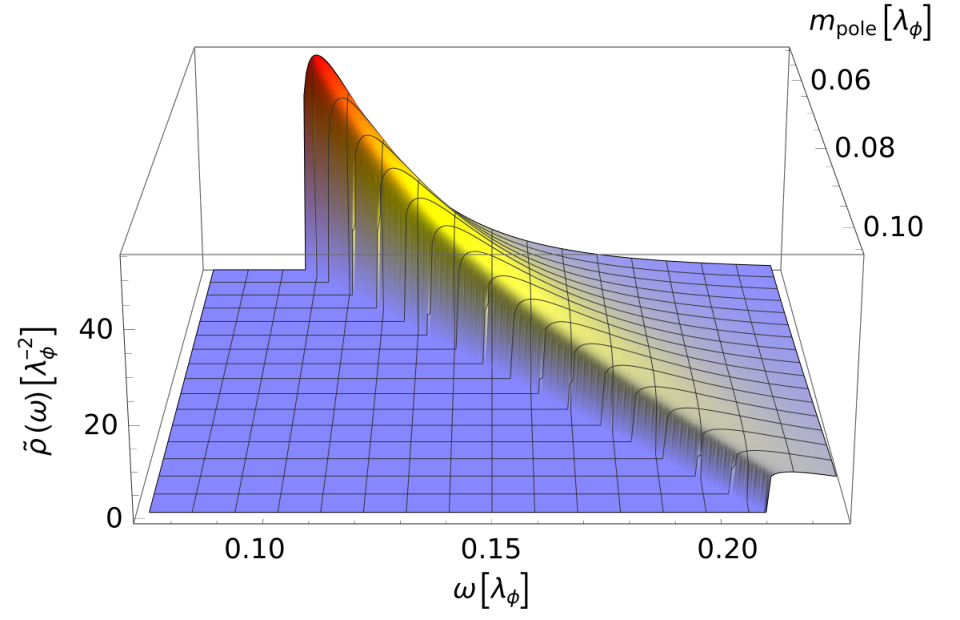
The scattering continuum sets in at $\lambda^{2}=m_{\text{\tiny{scat}}}^{2}$. In the case of a non-vanishing background field, the theory admits $1\to 2$ scattering (broken phase), and we have $m_{\text{\tiny{scat}}}=2m_{\text{\tiny{pole}}}$. Figure 1(a) shows the full scattering tail of the propagator as a function of the frequency $\omega$ and spatial momentum $|\vec{p}|$ in the broken phase. Higher thresholds of $1\rightarrow N$ scattering processes lead to further discontinuities in the scattering tail and are typically strongly suppressed. In the absence of $1\to 2$ scatterings (symmetric phase), the first allowed scattering is $1\to 3$ and the scattering threshold is $m_{\text{\tiny{scat}}}=3m_{\text{\tiny{pole}}}$, the respective spectral function is depicted in Figure 9 and discussed there.

If the spectral representation 2 holds, all non-analyticities of the propagator lie on the real frequency axis. These non-analyticities are given by either poles or cuts. Poles originate from asymptotic states that overlap with the propagator of the field $\phi$, while cuts represent scattering states.

For the propagator of a physical field that describes an asymptotic state, the spectral function is positive. Furthermore, the canonical commutation relations imply a normalisation via the sum rule,

$\displaystyle\int_{0_{-}}^{\infty}\frac{\mathrm{d}\lambda}{\pi}\,\lambda\,\rho(\lambda,\vec{p})=1\,,$

(4)

for all spatial momenta. Inserting the spectral function 3 into 4, we arrive at

$\displaystyle\frac{1}{Z_{\phi}}=1-\int_{m_{\text{\tiny{scat}}}}^{\infty}\frac{\mathrm{d}\lambda}{\pi}\,\lambda\,\tilde{\rho}(\lambda,\vec{p}\,)\,.$

(5)

Equation 5 comprises the well-known property that the on-shell amplitude $1/Z_{\phi}$ is bounded from above by unity, $Z_{\phi}\geq 1$, as the scattering tail carries part of the total probability.

Vertices also admit spectral representations, which get increasingly complicated for higher order correlation functions due to their increase in arguments. In the present case, we restrict ourselves to an $s$-channel approximation of the full one-particle irreducible (1PI) four-point function or vertex. This leaves us with a single momentum argument and an accordingly simple spectral representation. The four-point function is given by the fourth field derivative of the effective action $\Gamma[\phi]$, whose $n^{\text{th}}$ field derivatives $\Gamma^{(n)}[\phi]$ are the 1PI $n$-point functions. We use a spectral representation for this $s$-channel vertex Horak et al. 2020,

	$\displaystyle\Gamma^{(4)}(p_{0},\vec{p}\,)=$	$\displaystyle\,\lambda_{\phi}+\int_{\lambda}\frac{\rho_{4}(\lambda,\vec{p}\,)}{\lambda^{2}+p_{0}^{2}}\,,$
	$\displaystyle\rho_{4}(\omega,\vec{p}\,)=$	$\displaystyle\,2\,\text{Im}\,\Gamma^{(4)}(p_{0}=-\text{i}(\omega+\text{i}0^{+}),\vec{p}\,)\,,$		(6)

where $\lambda_{\phi}$ is the classical vertex in 1 and

$\displaystyle\int_{\lambda}=\int_{0_{-}}^{\infty}\frac{\mathrm{d}\lambda}{\pi}\lambda\,.$

(7)

Analogue to the spectral function of the propagator, $\rho_{4}$ is defined by the discontinuities of the four-point function, see 6. Also for the four-point function, the spatial momentum dependence of spectral function $\rho_{4}(\omega,\vec{p}\,)$ follows from the one at vanishing spatial momentum, $\rho_{4}(\omega)=\rho_{4}(\omega,0)$ via a Lorentz boost.

Figure 1(b) shows the spectrum of the four-point function in the $s$-channel approximation discussed in Section IV. It shows the $2\rightarrow 2$ scattering onset at twice the pole mass $m_{\text{\tiny{pole}}}$ of the field $\phi$. The next threshold from the $2\rightarrow 3$ scattering is also visible, but the result also contains the strongly suppressed threshold of higher order scattering processes. A more detailed discussion of our results is given in Section V.

In the spectral functional approach, spectral representations are utilised to rewrite diagrams in terms of momentum loop integrals over classical propagators with spectral masses and residual spectral integrals; for a general discussion see Horak et al. 2020. In the present work, we apply this approach in the context of the functional renormalisation group, amounting to the spectral fRG approach detailed in Section III. This leads to one-loop exact relations for correlation functions in terms of full propagators and vertices. In addition, we use a one-loop closed, resummed Bethe-Salpeter kernel to compute the four-point function.

As discussed above, the spectral fRG leads to perturbative one-loop momentum integrals in diagrams, which can be solved analytically. The non-perturbative information of the diagrams such as pole masses and thresholds is stored in the remaining spectral integrals. For the present purpose, it is sufficient to consider a single external momentum argument, which is either that of the propagator or the $s$-channel momentum of the four-point function. However, the generalisation to diagrams with several external momenta as present in the spectral computations of general $n$-point functions is straightforward.

In the present case, we only have to consider diagrams with one in-flowing or out-flowing external momentum $\pm p$, and we encounter diagrams of the general form

$\displaystyle D[p]=g\int_{q}\text{Vert}(p,q)\prod_{j=1}^{N}G(l_{j})\,,$

(8)

where $l_{i}=q,q\pm p$ are the momenta of the $N$ propagators and we have used the abbreviation

$\displaystyle\int_{q}=\int\frac{\mathrm{d}^{d}q}{(2\pi)^{d}}\,.$

(9)

$\text{Vert}(p,q)$ carries the momentum dependence of all vertices, which we assume to be either a polynomial or rational function of $p$ and the $l_{i}$, or to admit a spectral representation. All prefactors are collected in the overall prefactor $g$. By inserting the spectral representation 2 for each propagator, the momentum integrals acquire a standard perturbative form, where the masses are the respective spectral parameters squared, $\lambda_{i}^{2}$. Finally, the spectral parameters are integrated over, weighted by the respective spectral function,

$\displaystyle D[p]=g\prod_{j=1}^{N}\int_{\lambda_{j}}\rho(\lambda_{j})I(\lambda_{1},..,\lambda_{N},p)\,,$

(10)

with

$\displaystyle I(\lambda_{1},..,\lambda_{N},p)=\int_{q}\text{Vert}(p,q)\prod_{j=1}^{N}\frac{1}{\lambda_{j}^{2}+l_{j}^{2}}\,.$

(11)

The momentum integral in 11 is readily solved and the resulting analytic expression holds true for $p\,\in\,\mathbb{C}$. This gives us access to the spectral function 2 via the limit $p\rightarrow-\text{i}(\omega+\text{i}0^{+})$. We remark that in the present spectral fRG approach to the (1+2)-dimensional scalar theory, all integrals are finite, and we can safely change the order of integration even prior to renormalisation. In general the interchange of momentum and spectral integration performed in 10 assumes a suitable regularisation of the full integral, which can be done with spectral renormalisation Horak et al. 2020.

The spectral structure of the diagrams allows for a simple discussion of the emergent scattering thresholds that can be easily tracked within spectral functional approaches. An illustrative example is given by the contribution of the vacuum polarisation diagram to the spectral function of a single scalar field: It features a branch cut that opens at the sum of the spectral masses of the two propagators. The spectral function entering the diagram consists of a mass pole at $m_{\text{\tiny{pole}}}$ and a sum of scattering continua $\rho_{N}$ starting at $Nm_{\text{\tiny{pole}}}$ with $N\geq 2$. It follows straightforwardly from the analytic structure of that diagram that substituting scattering contributions $\rho_{N}$ and $\rho_{M}$ for the two internal lines directly yields a contribution to $\rho_{N+M}$. This demonstrates how any scattering structure, once seeded, gives rise to higher scattering contributions.

The infinitesimal change of the quantum effective action $\Gamma[\phi]$ under a change of the mass $\mu$ is governed by the manifestly finite renormalised Callan-Symanzik equation, Fehre et al. 2023; Braun et al. 2022,

	$\displaystyle\mu\partial_{\mu}\Gamma[\phi]=$	$\displaystyle\,\frac{1}{2}\,\left(1-\frac{\eta_{\phi}}{2}\right)Z_{\phi}\mu\,\text{Tr}\,\Bigl[\,G[\phi]+\phi^{2}\Bigr]$
		$\displaystyle\hskip 85.35826pt-\frac{1}{2}\,\mu\partial_{\mu}S_{\text{ct}}[\phi]\,,$		(14a)
with the anomalous dimension
	$\displaystyle\eta_{\phi}=-2\frac{\mu\partial_{\mu}\,Z_{\phi}}{Z_{\phi}}\,,$			(14b)
The factor 2 in 14b takes into account that $\mu$ has mass dimension 2. The argument $\phi$ in 14 is the mean field. The term $\mu\partial_{\mu}S_{\text{ct}}[\phi]$ in the second line of 14a is the flow of the counter terms that renders the flow equation finite, where the factor $1/2$ was added for convenience. The loop term on the right-hand side depends on the full field-dependent propagator. In the momentum basis it is given by
	$\displaystyle G[\phi](p,q)=$	$\displaystyle\,\langle\varphi\varphi\rangle_{c}(p,q)=\frac{1}{\Gamma^{(2)}[\phi]}(p,q)\,,$		(14c)
where the subscript c refers to the connected part of the two-point function and the mean field $\phi$ is given by the expectation value of the quantum field $\varphi$, i.e., $\phi=\langle\varphi\rangle$.

In the momentum basis, the trace in 14a corresponds to a momentum integral.

Note that the effective action $\Gamma[\phi]$ in 14 includes the full mass term $1/2\int_{x}\mu\,\phi^{2}$ in contradistinction to the effective action used in standard fRG momentum-shell flows. There, the momentum dependent regulator part of the mass term is subtracted, and the physical theory is reached when it vanishes. In the present setup, the $\mu$-dependent effective action is that of a physical theory with mass parameter $\mu$, and the flow is one in (physical) theory space. In contrast to usual momentum shell flows, this physical flow is both manifestly Lorentz invariant and sustains causality of physical correlation functions throughout the flow, allowing for the use of the Källén-Lehmann spectral representation 2.

Compared to the Wetterich equation, Wetterich 1993, with a momentum-dependent infrared regularisation, the novel ingredient in the functional Callan-Symanzik equation 14 is the explicit counter term flow $\mu\partial_{\mu}S_{\text{ct}}[\phi]$. The counter term flow has been derived in a manifestly finite limit of standard momentum cutoff flow equations as discussed in detail in Braun et al. 2022. The derivation entails that the flow of the counter term originates from a closed one-loop expression such as the trace in 14 itself, i.e., $\mu\partial_{\mu}S_{\text{ct}}[\phi]\sim\text{diagramms}$. Accordingly, the counter term flow contains no tree-level contributions to the respective correlation functions. This entails that classical values of the correlation functions are solely given by the respective choice of tree-level values specified in the classical action 12, and in particular cannot be further changed by specification of renormalisation conditions. In consequence, the latter can only be used to renormalise the flow contributions, but not the initial conditions of the flow. This excludes, for example, that the counter term flow rearranges the theory from the symmetric into the broken phase or vice versa by $\mu\partial_{\mu}S_{\textrm{ct}}\propto\pm\textrm{const.}\,\mu\int\phi^{2}$. However, the counter term can contain similar terms proportional to $\lambda_{\phi}/m_{\text{\tiny{pole}}}=\lambda_{\text{eff}}$.

In particular, the counter term flow allows for flowing renormalisation conditions, and we shall use it to adjust a flowing on-shell renormalisation, based on the spectral on-shell renormalisation put forward in Horak et al. 2020. Then, the pole mass $m_{\text{\tiny{pole}}}$ is identified with $m_{\phi}$ in 13 in both phases, $m_{\text{\tiny{pole}}}^{2}=\mu-3\mu\,\theta(-\mu)$. In this physical RG scheme, the phase transition between the symmetric and broken phase happens for $m^{2}_{\phi}=0$. Hence, we approach the phase transition both from the broken and the symmetric phase in the limit $\mu\to 0$, and the flows are taking place in the one or the other phase, see Figure 3. Thereby, our setup avoids flows through the strongly interacting phase transition regime, which are usually present in momentum cutoff flows. This minimises the systematic error stemming from the strong dynamics in the vicinity of a phase transition, where the flows are highly sensitive to truncation artefacts. However, it is in principle possible to flow through the phase transition, what can be advantageous if it is difficult to identify a proper starting point in one phase, at which the theory is particularly simple. An example for this situation can be found in quantum mechanics, where the theory for $\mu\to-\infty$ does not approach the classical limit but the instanton dominated regime.

In the present work, we consider the flow of the inverse propagator within the spectral representation. The flow is given by

	$\displaystyle\mu\partial_{\mu}\Gamma^{(2)}(p^{2})=$	$\displaystyle\,\left(1-\frac{\eta_{\phi}}{2}\right)Z_{\phi}\mu\,\left[D_{\text{\tiny{pol}}}(p^{2})-\frac{1}{2}D_{\text{\tiny{tad}}}(p^{2})\right]$
		$\displaystyle+\left(1-\frac{\eta_{\phi}}{2}\right)Z_{\phi}\mu-\frac{1}{2}\,\mu\partial_{\mu}S^{(2)}_{\text{ct}},$		(15)

where $D_{\text{tad}}$ and $D_{\text{pol}}$ refer to the tadpole and polarisation diagram, see Figure 5. Their general form, in terms of the spectral representation for the propagator and four-point function, is discussed in Appendix A. Moreover, all quantities in 15 depend on the chosen background $\phi$. For general spacetime dependent backgrounds $\phi(x)$ this would lead to $\Gamma^{(2)}[\phi](p,q)$. In the explicit computations we consider the background $\phi_{0}$, which is the constant solution of the equation of motion

$\displaystyle\left.\frac{\delta\Gamma[\phi]}{\delta\phi}\right|_{\phi=\phi_{0}}=0\,.$

(16)

With this physical choice for the background, the general field-dependent propagator 14c reduces to the physical propagator $G(p^{2})$ in the absence of source terms,

$\displaystyle G(p^{2})=\frac{1}{\Gamma^{(2)}[\phi_{0}](p^{2})}\,.$

(17)

In the symmetric phase, we have $\phi_{0}=0$, while $\phi_{0}\neq 0$ signals the broken phase. At constant fields the propagator 14c reduces to $G(p,q)=G(p^{2})(2\pi)^{d}\delta(p+q)$. Similarly we have $\Gamma^{(2)}[\phi_{0}](p,q)=\Gamma^{(2)}[\phi_{0}](p^{2})(2\pi)^{d}\delta(p+q)$.

In three dimensions the two phases are separated by a second order phase transition in the Ising universality class. From now on we drop the field argument $\phi_{0}$. It is implicitly understood that all correlation functions are evaluated at $\phi=\phi_{0}$.

In a final step, we substitute $\mu$ with $\pm k^{2}$, to keep the relations to standard fRG flows with momentum cutoffs simple, where $k$ is commonly used. This facilitates the comparison and benchmarking of the real-time results obtained with the spectral fRG. For example, the three dimensional $\phi^{4}$-theory has been studied abundantly within the Euclidean fRG, including systematic studies of the convergence of approximation schemes, for a recent review see Dupuis et al. 2021. These results carry over straightforwardly to the present approach, and the Euclidean correlation functions obtained from the spectral functions can be directly compared. This substitution leads us to

$\displaystyle k^{2}=|\mu|\,,\qquad\partial_{t}=k\,\partial_{k}=2\mu\partial_{\mu}\,\,,$

(18)

where the (negative) RG-time $t=\log(k/k_{\text{ref}})$ is measured relatively to a suitable reference scale or mass.

We proceed with discussing the on-shell spectral renormalisation, using the direct access to Minkowskian momenta. In (1+2)-dimensions, both diagrams in the CS flow 15 are manifestly finite, and the flow of the counter term action $\mu\partial_{\mu}S_{\text{ct}}$ only guarantees the implementation of the chosen renormalisation conditions. The (1+2)-dimensional $\phi^{4}$-theory is super-renormalisable, and one only has the renormalisation condition for the mass. Now we use on-shell renormalisation to keep the full pole mass on the classical input mass 13 with $m_{\text{\tiny{pole}}}^{2}=k^{2}$ in the symmetric phase, and $m_{\text{\tiny{pole}}}^{2}=2k^{2}$ in the broken phase. This leads us to

1. (i)

   symmetric phase:

   $\displaystyle\Gamma^{(2)}[\phi_{0}]\Big|_{p^{2}=-k^{2}}=0\,,$

   (19)

2. (ii)

   broken phase:

   $\displaystyle\Gamma^{(2)}[\phi_{0}]\Big|_{p^{2}=-2k^{2}}=0\,.$

   (20)

In the symmetric phase, the first allowed scattering process is the $1\to 3$ scattering, and the onset of the scattering continuum is located at three times the pole mass. In turn, in the broken phase with $1\rightarrow 2$ scattering, the onset of the scattering continuum of the spectral function is located at twice the pole mass. Thus, the spectral function 3 reads

$\displaystyle\rho(\lambda)=\frac{2\pi}{Z_{\phi}}\delta(\lambda^{2}-m_{\text{\tiny{pole}}}^{2})+\theta(\lambda^{2}-m^{2}_{\text{\tiny{scat}}})\tilde{\rho}(\lambda)\,,$

(21)

with $m_{\text{\tiny{scat}}}=3m_{\text{\tiny{pole}}}$ (symmetric phase) and $m_{\text{\tiny{scat}}}=2m_{\text{\tiny{pole}}}$ (broken phase). In Figure 2, we show the scale evolution of the spectral function $\rho$ in the broken phase: in Figure 2(a) we depict the scattering tail $\tilde{\rho}$, and in Figure 2(b) we depict the amplitude of the pole contribution. All quantities are measured relative to the coupling $\lambda_{\phi}$.

The spectral tail is rising towards smaller pole masses for a fixed classical coupling, and in turn the amplitude $1/Z_{\phi}$ of the pole contribution is decreasing. In combination the sum rule 4 holds during the evolution. The growing importance of the scattering processes can be understood from the fact that the dynamics of the theory only depend on the dimensionless ratio $\lambda_{\phi}/m_{\phi}$ with $m_{\phi}\propto k$. Hence, the effective coupling grows strong for smaller pole masses and on the other hand the dynamics of the theory are vanishing for asymptotically large pole masses.

In contrast to the Callan-Symanzik or mass regulator used in the present work, commonly used regulators in Euclidean flows decay for momenta larger than the IR cutoff $k$. This provides manifestly finite flows without the need of further renormalisation. Moreover, for Euclidean momenta, the respective flows of lower order correlation functions decay faster than for a CS regulator. In Minkowski space, however, the CS or mass regulator has the welcoming property, that the one-loop flow of $\rho(\omega)$ contains only classical correlation functions and is maximally local. While this is trivial in the symmetric phase where the one-loop flow only shifts the pole mass and does not generate a scattering continuum, it is non-trivial in the broken phase. There, the flow of the scattering continuum is given by a single delta function at the onset of the scattering spectrum, which originates from $\partial_{t}\,\text{Im}\,\Gamma^{(2)}\propto\delta(\omega^{2}-4m_{\text{\tiny{pole}}}^{2})$. Since the mass pole constitutes the dominant part of the propagator, the flow of the spectral function at spectral values larger than the flowing onset $2m_{\text{\tiny{pole}}}$, which is solely induced by the scattering tail, is sub-leading.

In general, the flow equation 14a can be evaluated for arbitrary values of the external field $\phi$, which requires the inclusion of the full effective potential. However, this goes beyond the scope of this work, and we simply evaluate the flow on the solution $\phi_{0}$ of the equation of motion 16. This is a commonly used truncation as it gives access to the physical correlation functions.

In the present fRG approach with the spectral CS regulator, the flow takes place in theory space and the effective action is physical for all values of $k$. In the broken phase, the minimum of the full effective potential depends on $k$, and the total mass flow of the two-point function is given by the flow diagrams originating from the CS equation, $\partial_{t}\Gamma^{(2)}[\phi_{0}](p)$ and a term proportional to the mass flow of $\phi_{0}$,

$\displaystyle\frac{d}{dt}\Gamma^{(2)}[\phi_{0}](p)=\partial_{t}\Gamma^{(2)}[\phi_{0}](p)+\left(\partial_{t}\phi_{0}\;\Gamma^{(3)}[\phi_{0}]\right)(p)\,.$

(22)

The novel ingredient in the present setup originates in the tree-level $k$-dependence of $\phi_{0}\approx\sqrt{6k^{2}/\lambda_{\phi}}+\mathcal{O}(\lambda_{\phi}k)$, where the second term comprises the loop corrections. This tree-level dependence is usually absent in the flow of the minimum in standard momentum-shell flows. There, $\partial_{t}\phi_{0}$ only comprises the effects of the momentum shell integration and hence is inherently one-loop and beyond. The tree-level $k$-dependence of $\phi_{0}$ in the present case triggers a tree-level $k$-dependence of $\partial_{t}\phi_{0}\Gamma^{(3)}(p)$ and the tree-level flow of the physical two-point function considered here reads

$\displaystyle\frac{d}{dt}\,\Gamma^{(2)}\Big|_{\text{\tiny{tree-level}}}$

$\displaystyle=-2k^{2}+\partial_{t}\phi_{0}S^{(3)}[\phi_{0}]=4k^{2}\,,$

(23)

where the classical three-point function is given by $S^{(3)}[\phi]=\lambda_{\phi}\phi$. Note that only the combination of both terms leads to the expected positive flow of the physical mass, while the flow of the mass parameter $-k^{2}$ has a negative sign.

To obtain the full momentum structure of the second term in of 22, we first note that the additional leg of the three-point function is always augmented with an incoming momentum of zero, as it is contracted with the scale derivative of a constant field. The full momentum dependence can then be incorporated via the DSE of the three-point function, which allows for an exact diagrammatic flow of the two-point function on the physical minimum. In the presence of approximations, a fully self-consistent treatment would require us to use the integrated flow of $\Gamma^{(3)}[\phi_{0}](p,0)$. However, also the flow of $\Gamma^{(3)}[\phi_{0}]$ includes a similar additional term as in 23, which is proportional to the four-point function. To avoid solving the flow of the three- and four-point function, we resort to the DSE to include the leading momentum dependence of the (contracted) three-point function. To ensure the correct RG-scaling of the flow equation, we further employ the skeleton expansion in the DSE, where every vertex is dressed. Approximating $\Gamma^{(n>4)}\approx 0$ and dropping the remaining two-loop diagrams, we arrive at the simple diagrammatic structure of the three-point function depicted in Figure 7.

Additionally, using the DSE for $\Gamma^{(3)}$ in 22 demonstrates the structure of the flow as a total derivative. To make this explicit, we choose the vertical leg in Figure 7 to be contracted with $\partial_{t}\phi_{0}$. Then, the three-point functions connected to this leg carry only internal momenta, and we approximate them as constant. With that, the first fish- and the triangle diagram in Figure 7 are proportional to the tadpole and polarisation diagram respectively, and the second term on the RHS of the flow 22 reads

	$\displaystyle\hskip-5.69054pt\Big(\partial_{t}\phi_{0}\;\Gamma^{(3)}[\phi_{0}]\Big)(p)=$	$\displaystyle\,\partial_{t}\phi_{0}\,\bigg(S^{(3)}[\phi_{0}]-\frac{1}{2}\Gamma^{(3)}[\phi_{0}]\,D_{\text{\tiny{tad}}}(p)$
		$\displaystyle\hskip-8.53581pt-D_{\text{\tiny{fish}}}(p)+\Gamma^{(3)}[\phi_{0}]\,D_{\text{\tiny{pol}}}(p)\bigg)\,.$		(24)

Note that the explicit three-point functions on the right-hand side are now momentum independent. For the full expressions of the spectral diagrams we refer to Appendix A. We discuss our approximations for the remaining vertices in Section IV.

Substituting 15 and III.3 into 22, we eventually arrive at the full flow equation of the two-point function. Its diagrammatic representation is depicted in Figure 6. It is illuminating to consider the one-loop structure of the flow, where the nature of the flow being a total derivative can be read off Figure 6. Then, the red crossed circle comprises the total derivative of the internal propagators in the (one-loop) polarisation and tadpole diagram, while the fish-diagram accounts for the running of the three-point vertices. The full equation reads

		$\displaystyle\hskip-3.98337pt\frac{d}{dt}\Gamma^{(2)}[\phi_{0}](p)=\;\left(\partial_{t}\phi_{0}\right)S^{(3)}[\phi_{0}]-\left(2-\eta_{\phi}\right)Z_{\phi}k^{2}$
		$\displaystyle\hskip 14.22636pt+\dot{\mathcal{R}}\left[-\frac{1}{2}D_{\text{\tiny{tad}}}+D_{\text{\tiny{pol}}}\right]-\partial_{t}\phi_{0}D_{\text{\tiny{fish}}}-\partial_{t}S_{\text{\tiny{ct}}}[\phi_{0}]\,,$		(25a)
where
	$\displaystyle\dot{\mathcal{R}}=\left(\partial_{t}\phi_{0}\Gamma^{(3)}[\phi_{0}]-\left(2-\eta_{\phi}\right)Z_{\phi}k^{2}\right)\,,$			(25b)

is represented as red crossed circle in Figure 6. Note the appearance of a relative minus sign in front of the mass derivative contribution (second term) to 25b due to $\mu=-k^{2}$ in the broken phase. The first line in 25a carries the trivial, tree-level running of inverse propagator. It consists of the running of the mass parameter and the classical part of the three-point function, connected to the flow of the minimum. Its mean-field value cannot be altered by the renormalisation condition and is, analogue to the respective term in $\dot{\mathcal{R}}$, crucial to recover the correct sign of the flow, see 23. A detailed evaluation of 25a can be found in Appendix B.

In the symmetric phase with $\phi_{0}=0$ in 16, we use a Taylor expansion about $\phi^{2}=0$ for the effective potential,

$\displaystyle V_{\textrm{eff}}(\phi)=\sum_{n=1}^{\infty}\frac{\lambda_{n}}{2n!}\phi^{2n}\,.$

(29)

The first two couplings, $\lambda_{1}$ and $\lambda_{2}$ are related to the correlation functions $\Gamma^{(2)}$ and $\Gamma^{(4)}$ considered here. Hence, the coupling $\lambda_{1}$ agrees with the curvature mass squared in the symmetric phase, where the curvature mass is defined as

$\displaystyle m_{\text{\tiny{curv}}}^{2}=V_{\textrm{eff}}^{(2)}(\phi_{0})=\Gamma^{(2)}[\phi_{0}](p=0)\,,$

(30)

in both phases. Moreover, the coupling $\lambda_{2}$ is nothing but the full four-point function, evaluated at vanishing momentum. In summary we have

$\displaystyle\lambda_{1}=m_{\text{\tiny{curv}}}^{2}\,,\qquad\lambda_{2}=\Gamma^{(4)}(p=0)\,.$

(31)

For the initial UV pole mass $m_{\text{\tiny{pole}}}=\Lambda$, the curvature mass and the pole mass agree, $\lambda_{1}=\Lambda^{2}$, and the initial coupling is the classical one, $\lambda_{2}=\lambda_{\phi}$. Hence, the initial effective potential $V_{\text{\tiny{UV}}}(\phi)$ at $k=\Lambda$ reads

$\displaystyle V_{\text{\tiny{UV}}}(\phi)=\frac{1}{2}\Lambda^{2}\phi^{2}+\frac{1}{4!}\lambda_{\phi}\,\phi^{4}\,.$

(32)

With the above approximations, all higher correlation functions are fixed and the flow equation of the two-point function on the real frequency axes reads

$\displaystyle\partial_{t}\Gamma^{(2)}(\omega_{+})$

$\displaystyle=-\frac{Z_{\phi}\left(2-\eta_{\phi}\right)k^{2}}{2}D^{\text{dyn}}_{\text{tad}}(\omega_{+})+2k^{2}-\partial_{t}\hat{S}_{\text{ct}}^{(2)},$

(33)

where the retarded limit is given by $\omega_{+}=-\text{i}(w+\text{i}0^{+})$ and is explicitly carried out in Appendix F. $\hat{S}^{(2)}_{\text{ct}}$ is given schematically by

$\displaystyle\hat{S}^{(2)}_{\text{ct}}=\text{diagramms}\left(p^{2}=-k^{2}\right)\,.$

(34)

We denoted the counterterm action with a tilde since we already dropped constant terms in the flow of order $\lambda_{\phi}k$. Hence, only the dynamic part of the tadpole $D^{\text{\tiny{dyn}}}_{\text{\tiny{tad}}}$ contributes. It arises from the scattering tail of $\Gamma^{(4)}(p)$ and carries the spectral structure of the polarisation diagram, see 47. In particular, the deviation of the constant term in Figure 5 from its classical value, $2k^{2}$, is of order $(\lambda_{\phi}k)$ and is therefore absorbed in the renormalisation constant. With that, 33 is consistent with the flowing on-shell renormalisation condition 19.

In the broken phase with $\phi_{0}\neq 0$ we use a Taylor expansion about $\phi^{2}=\phi_{0}^{2}$ for the effective potential,

$\displaystyle V_{\textrm{eff}}(\phi)=\sum_{n=2}^{\infty}\frac{\lambda_{n}}{2n!}\left(\phi^{2}-\phi_{0}^{2}\right)^{n}\,.$

(35)

At vanishing momentum and constant fields, the correlation functions derived from the effective action $\Gamma[\phi_{0}]$ coincide with the moments of the effective potential. We consider $n$-point functions for $n\leq 4$ with

		$\displaystyle\Gamma^{(2)}[\phi_{0}]\left(p=0\right)=\frac{1}{3}\lambda_{2}\phi_{0}^{2}\,,$
		$\displaystyle\Gamma^{(3)}[\phi_{0}]\left(p=0\right)=\,\lambda_{2}\,\phi_{0}+\frac{\lambda_{3}}{15}\,\phi_{0}^{3}\,,$
		$\displaystyle\Gamma^{(4)}[\phi_{0}]\left(p=0\right)=\lambda_{2}+\frac{2}{5}\lambda_{3}\,\phi_{0}^{2}+\frac{1}{105}\lambda_{4}\,\phi_{0}^{4}\,,$		(36)

In contrast to the symmetric phase discussed in Section IV.1, also higher order terms with couplings $\lambda_{n}$ contribute due to $\phi_{0}\neq 0$. For this reason we have indicated the $\phi_{0}$-dependence of $\Gamma^{(n)}$ in 36. As discussed below 17, we generically drop the $\phi_{0}$-dependence for the sake of readability, it is implicitly assumed that all expressions are evaluated at $\phi_{0}$.

As a consequence of 26, all expansion coefficients $\lambda_{n}$ with $n\geq 3$ vanish. The three and four-point couplings are then given by

$\displaystyle\Gamma^{(3)}(0)=\Gamma^{(4)}(0)\phi_{0}\,,\qquad\lambda_{2}=\Gamma^{(4)}(0)\,.$

(37)

With 30 we can express the minimum of the effective potential in terms of the curvature mass and $\lambda_{2}$, yielding

$\displaystyle\phi_{0}^{2}=\frac{3m_{\text{\tiny{curv}}}^{2}}{\Gamma^{(4)}(0)}\,,$

(38)

Using 38, the three-point function is expressed in terms of the full two- and four-point functions at vanishing momentum,

$\displaystyle\Gamma^{(3)}(0)=$

$\displaystyle\,\sqrt{3\,\Gamma^{(4)}(0)}\,m_{\text{\tiny{curv}}}\,.$

(39)

Evidently, in the classical limit with $Z_{\phi}=1$ and $\tilde{\rho}_{k}=0$, the curvature mass agrees with the pole mass. This limit is approached for asymptotically large pole masses, where the effective coupling $\lambda_{\phi}/m_{\text{\tiny{pole}}}$ tends towards zero. Hence, the ultraviolet effective potential $V_{\text{\tiny{UV}}}(\phi)$ with $k=\Lambda\to\infty$ is augmented with a classical dispersion with $\mu=-\Lambda^{2}$ and the initial (classical) coupling $\lambda_{2}=\lambda_{\phi}$,

$\displaystyle V_{\text{\tiny{UV}}}(\phi)=\frac{1}{4!}\lambda_{\phi}\left(\phi^{2}-\phi_{0}^{2}\right)^{2}\,,\qquad\phi_{0}^{2}=\frac{6\Lambda^{2}}{\lambda_{\phi}}\,,$

(40)

for $\phi^{2}\geq\phi_{0}^{2}$. The initial curvature and pole mass are given by

$\displaystyle m_{\text{\tiny{pole}}}^{2}=m_{\text{\tiny{curv}}}^{2}=2\Lambda^{2}\,.$

(41)

With these approximations, the real-time flow of the two-point function in the broken phase, derived in Appendix B, reads

	$\displaystyle\partial_{t}\Gamma^{(2)}(\omega_{+}^{2})=$	$\displaystyle\,\dot{\mathcal{R}}\left(\,D_{\text{\tiny{pol}}}(\omega_{+}^{2})-\frac{1}{2}D^{\text{\tiny{dyn}}}_{\text{\tiny{tad}}}(\omega_{+}^{2})\right)$
		$\displaystyle+A\,D_{\text{\tiny{fish}}}(\omega_{+}^{2})+4k^{2}-\partial_{t}\hat{S}^{(2)}_{\text{ct}}\,.$		(42)

The prefactors are given in 53 and $\hat{S}^{(2)}_{\text{ct}}$ is given by

$\displaystyle\hat{S}^{(2)}_{\text{ct}}=\text{diagramms}\left(p^{2}=-2k^{2}\right)\,.$

(43)

Additionally to the polarisation topology, we note that flow equation in the broken phase differs from that in the symmetric phase. The constant part of 42 carries an additional factor of 2. This resembles the additional factor 2 of the squared pole-mass in the broken phase compared to its symmetric phase counterpart. Also the prefactor of the tadpole diagram deviates from the symmetric case, since it includes the implicit $k$-dependence of the internal lines via the flowing physical minimum.

In both phases, we have a positive curvature mass $m_{\text{\tiny{curv}}}>0$ on the equation of motion $\phi_{0}$. Its value is related to the pole mass $m_{\text{\tiny{pole}}}=k$ in the symmetric, and $m_{\text{\tiny{pole}}}=2k$ in the broken phase. The difference between the flows is the existence of vertices $\Gamma^{(2n+1)}$ in the broken phase. They are proportional to sums of powers of $\phi_{0}$, see 36, and hence vanish in the symmetric phase. Specifically, the flow of the two-point function in the broken phase contains the diagrammatic topology of a vacuum polarisation, see Figure 6.

This leads us to the following structure: the CS flows are initiated deep in the symmetric and deep in the broken phase for large pole masses and a given classical coupling $\lambda_{\phi}$, see 32 and 40 respectively. For the broken phase this entails, that also the field expectation value at the initial scale is large as it scales with $\Lambda$, see 38 and 40. Then, the pole mass is successively lowered and for $k=0$ one reaches the phase transition point from both sides. In particular, the flows do not leave the broken or symmetric phase. This is in seeming contradiction to the standard fRG picture in a scalar theory, where flows in the broken phase may end up in the symmetric phase, and those in the symmetric phase end up deeper in the symmetric phase. This apparent contradiction is resolved by the fact, that $\phi_{0}$ in the standard fRG is defined from the subtracted EoM. There, the trivial cutoff flow, which is $\propto k^{2}\phi^{2}$, is subtracted from the effective potential, and one recovers physics only in the limit $k\rightarrow 0$.

In the symmetric phase with $\phi_{0}=0$ we are left with the tadpole diagram in the flow of the two-point function 15. The resummation 27 introduces a non-trivial momentum dependence to the four-point function and, in consequence, also to the tadpole diagram. This allows to calculate the propagator spectral function in the symmetric phase, i.e., at vanishing field value, where the polarisation diagram is absent. For the respective flow equation on the real frequency axes see 33. The resulting spectral function is shown in Figure 9. In the symmetric phase, the scattering continuum starts at $3m_{\text{\tiny{pole}}}$. As mentioned above, the dynamic tadpole contribution 47 carries the momentum structure of the polarisation diagram, resembling the $s$-channel structure of the four-vertex. Still, the onset of its imaginary part is at thrice the pole mass, since the bubble resummed vertex represents a series of $2\rightarrow 2$ scatterings which leads to a generic two-particle onset of $\rho_{4}$. The quantum corrections to the symmetric phase propagator are small compared to the broken phase. The amplitude on the mass pole is close to one compared to the respective values in the broken phase, see Table 1. This is expected, since the first dynamic contribution is of two-loop order and corresponds to the sunset topology.

In the broken phase the condensate is non-vanishing, $\phi_{0}\neq 0$. To compute the spectral function, the flow equation is evaluated on the real frequency axes see 42.

The $N$-particle onset positions of the spectral scattering tail are governed by the imaginary part of 42. For the polarisation diagrams, where only propagators come into play, the flow exhibits an onset at the sum of the two mass-poles. In contrast, the contribution of the tadpole leads to an onset at thrice the pole-mass, as the four-point spectral function only consists of a scattering continuum starting at $2m_{\text{\tiny{pole}}}$, cf. Figure 10(b). A more detailed discussion of the scattering onsets in general is found in Appendix F and specifically for the tadpole in Section V.1.

In  Figure 10(a) the spectral function from the current fRG approach is compared to spectral DSE results from Horak et al. 2020. Every quantity is measured relative to the respective pole mass to facilitate comparison with the DSE results. This allows to compare the relative magnitude of the scattering continua for different coupling strengths. For effective couplings $\lambda_{\phi}/m_{\text{\tiny{pole}}}\lesssim 20$, the spectral weight of the scattering continuum is sub-leading, as can be inferred from the combination of Figure 2(b) and the sum rule 5. The amplitudes of the pole contributions are listed in Table 1.

We find a remarkable agreement of both methods in the tested coupling range. For effective couplings $\lambda_{\phi}/m_{\text{\tiny{pole}}}\approx 20$, the deviations start growing, specifically at the thresholds. Deviations between both methods arise due to differences in the resummation structure of the two functional equations in the current truncation. The convergence of functional techniques for a large range of couplings is non-trivial and strengthens our confidence in spectral functional approaches.

In general, the tail of the propagator spectral function is enhanced for stronger couplings, while the residue of the mass pole decreases as the scattering states become more accessible due to the rising dimensionless interaction strength. The three- and higher $N$-particle onsets are graphically not visible in the full spectral functions of Figure 10(a), but present in the data. In the limit of large couplings we expect the three-particle onset to become more pronounced as the tadpole contribution becomes large.

The four-point spectral function shown in Figure 10(b) consists of only a negative scattering tail corresponding to a $2\rightarrow 2$ scattering process. For higher couplings, the three-particle onset becomes visible. The different suppression of higher $N$-particle thresholds in the propagator- and four-point spectrum are explained by dimensional analysis. While for the propagator spectral function, higher $N$-particle onsets are suppressed by their squared energy threshold, the four-point spectral function decays only with $\lambda^{-1}$, leading to a suppression linear in their respective energy thresholds. In both cases, four-particle or higher onsets are strongly suppressed, since they come with at least one additional loop each.

Figure 11 shows the Euclidean propagators corresponding to the spectral functions of Figure 10(a). As a cross-check, we compare the Euclidean propagator calculated from the spectral representation to the propagator directly obtained from the integrated Euclidean flow. We find the spectral representation to hold.

References

- Horak et al. (2020) J. Horak, J. M. Pawlowski, and N. Wink, Spectral functions in the -theory from the spectral DSE, Phys. Rev. D 102, 125016 (2020), arXiv:2006.09778 [hep-th] .
- Horak et al. (2021) J. Horak, J. Papavassiliou, J. M. Pawlowski, and N. Wink, Ghost spectral function from the spectral dyson-schwinger equation, Phys. Rev. D 104, 074017 (2021).
- Horak et al. (2022a) J. Horak, J. M. Pawlowski, and N. Wink, On the complex structure of Yang-Mills theory, (2022a), arXiv:2202.09333 [hep-th] .
- Horak et al. (2022b) J. Horak, J. M. Pawlowski, and N. Wink, On the quark spectral function in QCD, (2022b), arXiv:2210.07597 [hep-ph] .
- Kallen (1952) G. Kallen, On the definition of the Renormalization Constants in Quantum Electrodynamics, Helv. Phys. Acta 25, 417 (1952).
- Lehmann (1954) H. Lehmann, On the Properties of propagation functions and renormalization contants of quantized fields, Nuovo Cim. 11, 342 (1954).
- Braun et al. (2022) J. Braun et al., Renormalised spectral flows, (2022), arXiv:2206.10232 [hep-th] .
- Fehre et al. (2023) J. Fehre, D. F. Litim, J. M. Pawlowski, and M. Reichert, Lorentzian Quantum Gravity and the Graviton Spectral Function, Phys. Rev. Lett. 130, 081501 (2023), arXiv:2111.13232 [hep-th] .
- Gasenzer and Pawlowski (2008) T. Gasenzer and J. M. Pawlowski, Towards far-from-equilibrium quantum field dynamics: A functional renormalisation-group approach, Phys. Lett. B 670, 135 (2008), arXiv:0710.4627 [cond-mat.other] .
- Gasenzer et al. (2010) T. Gasenzer, S. Kessler, and J. M. Pawlowski, Far-from-equilibrium quantum many-body dynamics, Eur.Phys.J. C70, 423 (2010), arXiv:1003.4163 [cond-mat.quant-gas] .
- Floerchinger (2012) S. Floerchinger, Analytic Continuation of Functional Renormalization Group Equations, JHEP 1205, 021, arXiv:1112.4374 [hep-th] .
- Kamikado et al. (2014) K. Kamikado, N. Strodthoff, L. von Smekal, and J. Wambach, Real-Time Correlation Functions in the O(N) Model from the Functional Renormalization Group, Eur.Phys.J. C74, 2806 (2014), arXiv:1302.6199 [hep-ph] .
- Tripolt et al. (2014) R.-A. Tripolt, N. Strodthoff, L. von Smekal, and J. Wambach, Spectral Functions for the Quark-Meson Model Phase Diagram from the Functional Renormalization Group, Phys. Rev. D89, 034010 (2014), arXiv:1311.0630 [hep-ph] .
- Pawlowski and Strodthoff (2015) J. M. Pawlowski and N. Strodthoff, Real time correlation functions and the functional renormalization group, Phys. Rev. D92, 094009 (2015), arXiv:1508.01160 [hep-ph] .
- Kamikado et al. (2017) K. Kamikado, T. Kanazawa, and S. Uchino, Mobile impurity in a Fermi sea from the functional renormalization group analytically continued to real time, Phys. Rev. A95, 013612 (2017), arXiv:1606.03721 [cond-mat.quant-gas] .
- Jung et al. (2017) C. Jung, F. Rennecke, R.-A. Tripolt, L. von Smekal, and J. Wambach, In-Medium Spectral Functions of Vector- and Axial-Vector Mesons from the Functional Renormalization Group, Phys. Rev. D95, 036020 (2017), arXiv:1610.08754 [hep-ph] .
- Pawlowski et al. (2018) J. M. Pawlowski, N. Strodthoff, and N. Wink, Finite temperature spectral functions in the O(N)-model, Phys. Rev. D98, 074008 (2018), arXiv:1711.07444 [hep-th] .
- Wang and Zhuang (2017) Z. Wang and P. Zhuang, Meson spectral functions at finite temperature and isospin density with the functional renormalization group, Phys. Rev. D96, 014006 (2017), arXiv:1703.01035 [hep-ph] .
- Tripolt et al. (2019) R.-A. Tripolt, C. Jung, N. Tanji, L. von Smekal, and J. Wambach, In-medium spectral functions and dilepton rates with the Functional Renormalization Group, Proceedings, 27th International Conference on Ultrarelativistic Nucleus-Nucleus Collisions (Quark Matter 2018): Venice, Italy, May 14-19, 2018, Nucl. Phys. A982, 775 (2019), arXiv:1807.04952 [hep-ph] .
- Tripolt et al. (2018) R.-A. Tripolt, J. Weyrich, L. von Smekal, and J. Wambach, Fermionic spectral functions with the Functional Renormalization Group, Phys. Rev. D98, 094002 (2018), arXiv:1807.11708 [hep-ph] .
- Corell et al. (2021) L. Corell, A. K. Cyrol, M. Heller, and J. M. Pawlowski, Flowing with the temporal renormalization group, Phys. Rev. D 104, 025005 (2021), arXiv:1910.09369 [hep-th] .
- Huelsmann et al. (2020) S. Huelsmann, S. Schlichting, and P. Scior, Spectral functions from the real-time functional renormalization group, Phys. Rev. D 102, 096004 (2020), arXiv:2009.04194 [hep-ph] .
- Jung et al. (2021) C. Jung, J.-H. Otto, R.-A. Tripolt, and L. von Smekal, Self-consistent O(4) model spectral functions from analytically continued functional renormalization group flows, Phys. Rev. D 104, 094011 (2021), arXiv:2107.10748 [hep-ph] .
- Tan et al. (2022) Y.-y. Tan, Y.-r. Chen, and W.-j. Fu, Real-time dynamics of the scalar theory within the fRG approach, SciPost Phys. 12, 026 (2022), arXiv:2107.06482 [hep-ph] .
- Heller and Pawlowski (2021) M. Heller and J. M. Pawlowski, Causal Temporal Renormalisation Group Flow of the Energy-Momentum Tensor, (2021), arXiv:2112.12652 [hep-th] .
- Roth et al. (2022) J. V. Roth, D. Schweitzer, L. J. Sieke, and L. von Smekal, Real-time methods for spectral functions, Phys. Rev. D 105, 116017 (2022), arXiv:2112.12568 [hep-ph] .
- Roth and von Smekal (2023) J. V. Roth and L. von Smekal, Critical dynamics in a real-time formulation of the functional renormalization group, (2023), arXiv:2303.11817 [hep-ph] .
- Wetterich (1993) C. Wetterich, Exact evolution equation for the effective potential, Phys. Lett. B301, 90 (1993), arXiv:1710.05815 [hep-th] .
- Dupuis et al. (2021) N. Dupuis, L. Canet, A. Eichhorn, W. Metzner, J. M. Pawlowski, M. Tissier, and N. Wschebor, The nonperturbative functional renormalization group and its applications, Phys. Rept. 910, 1 (2021), arXiv:2006.04853 [cond-mat.stat-mech] .
- Caselle et al. (2002) M. Caselle, M. Hasenbusch, P. Provero, and K. Zarembo, Bound states and glueballs in three-dimensional Ising systems, Nucl. Phys. B 623, 474 (2002), arXiv:hep-th/0103130 .
- Agostini et al. (1997) V. Agostini, G. Carlino, M. Caselle, and M. Hasenbusch, The Spectrum of the (2+1)-dimensional gauge Ising model, Nucl. Phys. B 484, 331 (1997), arXiv:hep-lat/9607029 .
- Caselle et al. (1999) M. Caselle, M. Hasenbusch, and P. Provero, Nonperturbative states in the 3-D phi**4 theory, Nucl. Phys. B 556, 575 (1999), arXiv:hep-lat/9903011 .
- Rose et al. (2016) F. Rose, F. Benitez, F. Léonard, and B. Delamotte, Bound states of the 4 model via the nonperturbative renormalization group, Phys. Rev. D 93, 125018 (2016), arXiv:1604.05285 [cond-mat.stat-mech] .
- Braun et al. (2023) J. Braun, Y.-r. Chen, W.-j. Fu, F. Gao, F. Ihssen, A. Geissel, J. Horak, C. Huang, Y. Lu, J. M. Pawlowski, F. Rennecke, F. Sattler, B. Schallmo, J. Stoll, Y.-y. Tan, S. Töpfel, J. Turnwald, R. Wen, J. Wessely, N. Wink, S. Yin, and N. Zorbach, fQCD collaboration, (2023).
- Bonanno et al. (2022) A. Bonanno, T. Denz, J. M. Pawlowski, and M. Reichert, Reconstructing the graviton, SciPost Phys. 12, 001 (2022), arXiv:2102.02217 [hep-th] .
- (36) W. R. Inc., Mathematica, Version 13.1, champaign, IL, 2022.
- Rajantie (1996) A. K. Rajantie, Feynman diagrams to three loops in three-dimensional field theory, Nucl. Phys. B 480, 729 (1996), [Erratum: Nucl.Phys.B 513, 761–762 (1998)], arXiv:hep-ph/9606216 .