跳到论文正文
W Papers独立论文阅读器 arXiv:2303.16385 论文正文 计算阅读时间 · 0%
引用这篇论文根据当前论文元数据生成,正式投稿前建议核对。


License: CC BY-NC-SA 4.0
arXiv:2303.16385v2 [cs.GT] 03 Jun 2023

Geometric Convergence of Distributed Heavy-Ball Nash Equilibrium Algorithm over Time-Varying Digraphs with Unconstrained ActionsThanks: The authors are with the School of Electrical, Computer and Energy Engineering, Arizona State University, Tempe, AZ, United States. Email: {dtnguy52, duongnt, Angelia.Nedich}@asu.edu. This material is based in part upon work supported by the NSF award CCF-2106336. Corresponding Author: Duong Thuy Anh Nguyen.

Duong Thuy Anh Nguyen       Duong Tung Nguyen    Affiliation: and Angelia Nedić,
Abstract

This paper presents a new distributed algorithm that leverages heavy-ball momentum and a consensus-based gradient method to find a Nash equilibrium (NE) in a class of non-cooperative convex games with unconstrained action sets. In this approach, each agent in the game has access to its own smooth local cost function and can exchange information with its neighbors over a communication network. The main novelty of our work is the incorporation of heavy-ball momentum in the context of non-cooperative games that operate on fully-decentralized, directed, and time-varying communication graphs, while also accommodating non-identical step-sizes and momentum parameters. Overcoming technical challenges arising from the dynamic and asymmetric nature of mixing matrices and the presence of an additional momentum term, we provide a rigorous proof of the geometric convergence to the NE. Moreover, we establish explicit bounds for the step-size values and momentum parameters based on the characteristics of the cost functions, mixing matrices, and graph connectivity structures. We perform numerical simulations on a Nash-Cournot game to demonstrate accelerated convergence of the proposed algorithm compared to that of the existing methods.

I Introduction

Nash equilibrium (NE) computation is essential for examining decision-making and strategic behavior in multi-agent systems, especially in non-cooperative games. These games have applications in numerous engineering domains, including electricity markets, power systems, flow control, and crowdsourcing [1, 2]. In non-cooperative games, each agent has their own goals and seeks to maximize their payoff, without coordinating with other agents. Classical complete information game theory typically employs best-response or gradient-based methods to find an NE, but these approaches necessitate each agent having complete information regarding the actions of its competitors [3, 4], which can be unrealistic in many practical engineering systems.

Extensive research has been conducted to develop efficient distributed methods for seeking NE in the settings with partial information available to the agents. These methods are primarily built upon projected gradient and consensus dynamics approaches, and they have been studied in both continuous-time [5] and discrete-time [6, 7] domains. Early works only consider time-invariant undirected networks, such as for example [8], which develops an algorithm within the framework of an inexact-ADMM. The accelerated gradient play algorithm (Acc-GRANE) presented in [9] is based on the strong monotonicity of an augmented mapping and is applicable to a subclass of games. Reference [10] extends the applicability of the Acc-GRANE algorithm to a broader class of games by assuming the restricted strong monotonicity of the augmented mapping. Based on the contraction properties of doubly stochastic matrices, reference [7] develops a distributed gradient method whose convergence properties do not depend on an augmented mapping.

There has been a growing interest in studying NE computation in communication networks with switching topologies. Early work [6] focuses on aggregative games over undirected graphs, while [11] extends the study to games with coupling constraints. Reference [12] proposes an asynchronous gossip algorithm for a directed graph, assuming each agent can update all estimates of the agents who interfere with its cost function. In [13], a projected pseudo-gradient-based algorithm is proposed for time-varying directed graphs that are weight-balanced, while [14] relaxes the weight-balancedness assumption for a static directed graph, assuming complete knowledge of the underlying communication graph. In [15], these assumptions are further relaxed, and a condition is established to address the loss of monotonicity with weighted norms, which is a commonly encountered issue. In [16], a robust algorithm is proposed that utilizes an observation graph allowing for direct observation of actions and, thus, making it immune to tampering by adversarial agents.

Most of the above mentioned works deal with gradient-based methods. The heavy-ball method, introduced in [17], has been widely used as an acceleration technique for gradient-based methods to achieve faster convergence [18]. In the context of aggregative games, the heavy-ball method has been employed in algorithms for both undirected [19] and directed [20] graphs, achieving convergence for diminishing step-sizes. It has also been employed in semi-decentralized communication architectures, where a central coordinator collects and transmits aggregative signals to the agents in the system [21]. Reference [22] considers games over undirected graphs with affine coupling constraints and introduces acceleration schemes for the proximal-point algorithm, such as (alternated) inertia and overrelaxation.

Contributions. Motivated by the potential benefits of the heavy-ball method in accelerating convergence, this paper presents a novel distributed, discrete-time algorithm for NE seeking by integrating the heavy-ball momentum and consensus-based gradient method. The proposed algorithm is designed to work on a general sequence of time-varying directed graphs, without requiring any coordination among agents for the weights. It also allows for non-identical step-sizes and momentum parameters. The incorporation of agent-based heavy-ball momentum terms introduces additional technical complexity in the convergence analysis of the algorithm. The main challenge is in ensuring the contraction properties of a recurrence relation due to the presence of the additional momentum terms, especially when dealing with time-varying asymmetric mixing matrices. Prior heavy-ball algorithms, such as those presented in [19] and [20] for aggregative games, utilize diminishing step-sizes to demonstrate that the state difference resulting from the additional momentum term converges to zero. Unfortunately, this approach is not applicable to this work since our algorithm employs a constant step-size rule. To overcome this technical challenge, we analyze three distinct quantities: the consensus error, the NE gap, and consecutive states difference. By establishing a composite relation for the vector comprising these quantities, we rigorously prove the linear convergence of the algorithm to the NE under strong monotonicity and Lipschitz continuity assumptions. We also provide explicit bounds for the constant step-size values and momentum terms based on the properties of the cost functions, mixing matrices, and graph connectivity structures.

This paper is structured as follows. Section II presents the problem formulation. In Section III, the distributed algorithm is introduced. Section IV provides convergence analysis and Section V numerically evaluates the performance of the proposed algorithm. Section VI concludes with key points.

Notations. All vectors are column vectors unless otherwise stated. We write u𝖳u^{\mathsf{T}} for the transpose of a vector u∈ℝnu\in{\mathbb{R}}^{n}. We use 𝟎{\mathbf{0}} and 𝟏{\mathbf{1}} to denote the vector with all entries equal to 00 and 11, respectively. The ii-th entry of a vector uu is denoted by uiu_{i}, while it is denoted by [uk]i[u_{k}]_{i} for a time-varying vector uku_{k}. We denote min⁡(u)=mini⁡ui\min(u)=\min_{i}u_{i} and max⁡(u)=maxi⁡ui\max(u)=\max_{i}u_{i}. Given a vector uu, Diag⁡(u){\mathrm{Diag}}(u) denotes the diagonal matrix whose diagonal entries correspond to the entries of uu. A nonnegative vector is called stochastic if its entries sum up to 11.

We use Ai​jA_{ij} to denote the i​jij-th entry of a matrix AA, and [Ak]i​j[A_{k}]_{ij} when the matrix is time-dependent. The notation A≤BA\leq B is used when Ai​j≤Bi​jA_{ij}\leq B_{ij} for all i,ji,j, where AA and BB are matrices of the same dimension. A matrix AA is nonnegative if all its entries are nonnegative and min+⁡(A){\min}^{+}(A) denotes the smallest positive entry of AA. A nonnegative matrix A∈ℝn×nA\in\mathbb{R}^{n\times n} is row-stochastic if A​𝟏=𝟏A\mathbf{1}=\mathbf{1}. A consensual matrix has equal row vectors. The identity matrix is denoted by 𝕀\mathbb{I}. Given a vector π∈ℝm\pi\in{\mathbb{R}}^{m} with positive entries, we denote

⟨𝐮,𝐯⟩π=∑i=1mπi​⟨ui,vi⟩{\langle}{\mathbf{u}},{\mathbf{v}}{\rangle}_{\pi}=\sum_{i=1}^{m}\pi_{i}{\langle}u_{i},v_{i}{\rangle} and ‖𝐮‖π=∑i=1mπi​‖ui‖2,\|{\mathbf{u}}\|_{\pi}=\sqrt{\sum_{i=1}^{m}\pi_{i}\|u_{i}\|^{2}},

where 𝐮:=[u1,…,um]𝖳,𝐯:=[v1,…,vm]𝖳∈ℝm×n{\mathbf{u}}\!:=\![u_{1},\ldots,u_{m}]^{\mathsf{T}},{\mathbf{v}}\!:=\![v_{1},\ldots,v_{m}]^{\mathsf{T}}\!\!\in\!{\mathbb{R}}^{m\times n}, and ui,vi∈ℝnu_{i},v_{i}\!\in\!{\mathbb{R}}^{n}. When π=𝟏\pi={\mathbf{1}}, we write ⟨𝐮,𝐯⟩{\langle}{\mathbf{u}},{\mathbf{v}}{\rangle} and ‖𝐮‖\|{\mathbf{u}}\|. We have

1max⁡(π)​‖𝐮‖π≤‖𝐮‖≤1min⁡(π)​‖𝐮‖π,\displaystyle\tfrac{1}{\sqrt{\max(\pi)}}\|{\mathbf{u}}\|_{\pi}\leq\|{\mathbf{u}}\|\leq\tfrac{1}{\sqrt{\min(\pi)}}\|{\mathbf{u}}\|_{\pi}, (1)

and ⟨𝐮,𝐯⟩π≤‖𝐮‖π​‖𝐯‖π{\langle}{\mathbf{u}},{\mathbf{v}}{\rangle}_{\pi}\leq\|{\mathbf{u}}\|_{\pi}\|{\mathbf{v}}\|_{\pi} (Cauchy–Schwarz inequality).

We let [m]={1,…,m}[m]=\{1,\ldots,m\} for an integer m≥1m\geq 1. Given a directed graph 𝔾=([m],𝖤){\mathbb{G}}=([m],{\mathsf{E}}), specified by the set of edges 𝖤⊆[m]×[m]{\mathsf{E}}\subseteq[m]\times[m] of ordered pairs of nodes, the in-neighbor and out-neighbor set for every agent ii are defined, as follows:

𝒩iin={j∈[m]|(j,i)∈𝖤}​and​𝒩iout={ℓ∈[m]|(i,ℓ)∈𝖤}.{\mathcal{N}^{\rm in}_{i}}=\{j\!\in\![m]|(j,i)\!\in\!{\mathsf{E}}\}\!\!\!\text{and}\!\!\!{\mathcal{N}^{\rm out}_{i}}=\{\ell\!\in\![m]|(i,\ell)\!\in\!{\mathsf{E}}\}.

A directed graph 𝔾{\mathbb{G}} is strongly connected if there is a directed path from any node to all other nodes in 𝔾{\mathbb{G}}. We use 𝖣⁡(𝔾)\mathsf{D}({\mathbb{G}}) and 𝖪⁡(𝔾)\mathsf{K}({\mathbb{G}}) to denote the diameter and the maximal edge-utility of a strongly connected directed graph 𝔾{\mathbb{G}}, respectively, as defined in Definition 2.1 and Definition 2.2 in [23].

II Problem Formulation

We study a non-cooperative game with mm agents, where each agent has an unconstrained action set Xi=ℝniX_{i}={\mathbb{R}}^{n_{i}}, for i∈[m]i\in[m]. Each agent ii has a cost function Ji​(xi,x−i)J_{i}(x_{i},x_{-i}) that depends on its own action xi∈Xix_{i}\in X_{i} and the joint action of all other agents except itself, x−i∈X−i=ℝn−nix_{-i}\in X_{-i}={\mathbb{R}}^{n-n_{i}}. The joint action vector of all agents has size n=∑i=1mnin=\sum_{i=1}^{m}n_{i} and belongs to the joint action set X=X1×⋯×Xm=ℝnX=X_{1}\times\cdots\times X_{m}={\mathbb{R}}^{n}. We assume that the cost function Ji​(xi,x−i)J_{i}(x_{i},x_{-i}) is continuously differentiable in xix_{i} for any fixed x−i∈X−ix_{-i}\in X_{-i}, for all i∈[m]i\in[m].

Denote the game by Γ=([m],{Ji},{Xi})\Gamma=([m],\{J_{i}\},\{X_{i}\}). A vector x∗=[x1∗,…,xm∗]𝖳∈Xx^{*}=[x_{1}^{*},\ldots,x_{m}^{*}]^{\mathsf{T}}\in X is a NE to the game Γ\Gamma if, for every agent i∈[m]i\in[m], the condition below is satisfied:

Ji​(xi∗,x−i∗)≤Ji​(xi,x−i∗),for all ​xi∈Xi.\displaystyle J_{i}(x_{i}^{*},x_{-i}^{*})\leq J_{i}(x_{i},x_{-i}^{*}),\quad\hbox{for all }x_{i}\in X_{i}. (2)

We define the game mapping F⁡(x):X→ℝnF(x):X\to{\mathbb{R}}^{n} as

F⁡(x)≜[∇1J1​(x1,x−1),…,∇mJm​(xm,x−m)]𝖳,\displaystyle F(x)\triangleq\left[\nabla_{1}J_{1}(x_{1},x_{-1}),\ldots,\nabla_{m}J_{m}(x_{m},x_{-m})\right]^{\mathsf{T}}, (3)

where ∇iJi​(xi,x−i)=∇xiJi​(xi,x−i)\nabla_{i}J_{i}(x_{i},x_{-i})=\nabla_{x_{i}}J_{i}(x_{i},x_{-i}) for all i∈[m]i\in[m].

We make the following assumptions.

Assumption 1

The game mapping F⁡(x)F(x) is strongly monotone on XX with the constant μ>0\mu>0.

Assumption 2

Consider the game Γ=([m],{Ji},{Xi})\Gamma=([m],\{J_{i}\},\{X_{i}\}), assume for all i∈[m]i\in[m]:
(a) The mapping ∇iJi​(xi,⋅)\nabla_{i}J_{i}(x_{i},\cdot) is Lipschitz continuous on X−iX_{-i} for every fixed xi∈Xix_{i}\in X_{i} with a uniform constant L−i>0L_{-i}>0.
(b) The mapping ∇iJi​(⋅,x−i)\nabla_{i}J_{i}(\cdot,x_{-i}) is Lipschitz continuous on XiX_{i} for every fixed x−i∈X−ix_{-i}\in X_{-i} with a uniform constant Li>0L_{i}>0.

Remark 1

Assumption 1 implies strong convexity of each cost function Ji​(xi,x−i)J_{i}(x_{i},x_{-i}) on XiX_{i} for every x−i∈X−ix_{-i}\in X_{-i} with the constant μ\mu, as noted in Remark 1 of [9]. The existence and uniqueness of a NE for the game Γ=([m],Ji,Xi)\Gamma=([m],{J_{i}},{X_{i}}) is also guaranteed by Assumption 1. This result is established in Theorem 2.3.3 of [24]. Moreover, as Xi=ℝniX_{i}={\mathbb{R}}^{n_{i}} for all i∈[m]i\in[m], x∗∈Xx^{*}\in X is the NE if and only if F⁡(x∗)=𝟎F(x^{*})={\mathbf{0}}.

III Distributed Nash Equilibrium Seeking

Consider a game Γ=([m],Ji,Xi)\Gamma=([m],{J_{i}},{X_{i}}) where agents interact through a sequence of time-varying communication graphs 𝔾k=([m],𝖤k){\mathbb{G}}_{k}=([m],{\mathsf{E}}_{k}) at time kk. Each link (j,i)(j,i) in 𝖤k{\mathsf{E}}_{k} indicates that agent ii receives information from agent jj. The graph is assumed to have self-loops for every node in each 𝔾k{\mathbb{G}}_{k}, ensuring that 𝒩i​kin{\mathcal{N}^{\rm in}_{ik}} and 𝒩i​kout{\mathcal{N}^{\rm out}_{ik}} always contain agent ii. The details are outlined in the following assumption.

Assumption 3

Each graph 𝔾k=([m],𝖤k){\mathbb{G}}_{k}=([m],{\mathsf{E}}_{k}) is strongly connected and has a self-loop at every node i∈[m]i\in[m].

Remark 2

Assumption 3 can be relaxed by considering BB-strongly-connected graph sequence, i.e., when an integer B≥1B\geq 1 exists such that the graph with edge set 𝖤kB=⋃i=k​B(k+1)​B−1𝖤i{\mathsf{E}}^{B}_{k}=\bigcup_{i=kB}^{(k+1)B-1}{\mathsf{E}}_{i} is strongly connected for every k≥0k\geq 0.

To deal with the partial information available to agents, each agent ii maintains a local variable zik=(zi​1k,…,zi​mk)𝖳∈ℝnz_{i}^{k}=(z_{i1}^{k},\ldots,z_{im}^{k})^{\mathsf{T}}\in{\mathbb{R}}^{n}, where zi​jkz_{ij}^{k} is agent ii’s estimate of the decision xjkx_{j}^{k} for agent j≠ij\neq i, while zi​ik=xikz_{ii}^{k}=x_{i}^{k}. The estimate of agent jj without the ii-th block-component is defined as

zj,−ik=(zj​1k,…,zj,i−1k,zj,i+1k,…,zj​mk)𝖳∈ℝn−ni.z_{j,-i}^{k}=(z_{j1}^{k},\ldots,z_{j,i-1}^{k},z_{j,i+1}^{k},\ldots,z_{jm}^{k})^{\mathsf{T}}\in{\mathbb{R}}^{n-n_{i}}.

Given the constraints on agents’ access to others’ actions in game Γ\Gamma, we propose a fully-distributed algorithm that respects the information access as dictated by the communication graphs 𝔾k{\mathbb{G}}_{k}. The approach, outlined in Algorithm 1, incorporates a gradient method with heavy-ball momentum. At each time kk, each agent ii sends its estimate zikz_{i}^{k} to its out-neighbors ℓ∈𝒩i​kout\ell\in{\mathcal{N}^{\rm out}_{ik}} and receives estimates zjkz_{j}^{k} from its in-neighbors j∈𝒩i​kinj\in{\mathcal{N}^{\rm in}_{ik}}. Agent ii then updates its own action xik+1x_{i}^{k+1} and local estimate zik+1z_{i}^{k+1} using the received information.

Algorithm 1: DNE-HB
Every agent i∈[m]i\in[m] selects a local stepsize αi>0\alpha_{i}>0, a
local momentum parameter βi>0\beta_{i}>0 and initializes with
arbitrary initial vectors zi,−i0∈ℝn−ni,xi0,xi−1∈ℝniz_{i,-i}^{0}\in{\mathbb{R}}^{n-n_{i}},x_{i}^{0},x_{i}^{-1}\in{\mathbb{R}}^{n_{i}}.
for k=0,1,…,k=0,1,\ldots, every agent i∈[m]i\in[m] does the following:
Receives zjkz_{j}^{k} from in-neighbors j∈𝒩i​kinj\in{\mathcal{N}^{\rm in}_{ik}};
Sends zikz_{i}^{k} to out-neighbors ℓ∈𝒩i​kout\ell\in{\mathcal{N}^{\rm out}_{ik}};
Chooses the weights [Wk]i​j,j∈[m][W_{k}]_{ij},j\in[m];
Updates the action xik+1x_{i}^{k+1} and estimates zi,−ik+1z_{i,-i}^{k+1} by
     xik+1=∑l=1m[Wk]i​l​zl​ik−αi​∇iJi​(∑j=1m[Wk]i​j​zjk)x_{i}^{k+1}=\sum_{l=1}^{m}[W_{k}]_{il}z_{li}^{k}-\alpha_{i}\nabla_{i}J_{i}\!\left(\sum_{j=1}^{m}[W_{k}]_{ij}z_{j}^{k}\right)
    +βi​(xik−xik−1)\qquad~~~~+\beta_{i}(x_{i}^{k}-x_{i}^{k-1});  zi,ik+1=xik+1z_{i,i}^{k+1}=x_{i}^{k+1};
     zi,−ik+1=∑j=1m[Wk]i​j​zj,−ik+βi​(zi,−ik−zi,−ik−1)z_{i,-i}^{k+1}=\sum_{j=1}^{m}[W_{k}]_{ij}z_{j,-i}^{k}+\!\beta_{i}(z_{i,-i}^{k}\!-z_{i,-i}^{k-1});
end for

We make the following assumption on the matrices WkW_{k}.

Assumption 4

For each k≥0k\geq 0, the weight matrix WkW_{k} is row-stochastic and compatible with the graph 𝔾k{\mathbb{G}}_{k} i.e.,

{[Wk]i​j>0,whenj∈𝒩ini​k,[Wk]i​j=0,otherwise.\displaystyle\begin{cases}[W_{k}]_{ij}>0,\quad\text{when}j\in{\mathcal{N}^{\rm in}_{ik}},\\ [W_{k}]_{ij}=0,\quad\text{otherwise.}\end{cases} (4)

There exist a scalar w>0w\!>\!0 such that min+⁡(Wk)≥w,∀k≥0\min^{+}(W_{k})\geq w,\forall k\geq 0.

IV Geometric Convergence of DNE-HB

IV-A Preliminaries

We outline basic results on norm of linear combinations of vectors, graphs, stochastic matrices, and gradient method.

Lemma 1 (​​[15], Corollary 5.2)

Consider a vector collection {ui,i∈[n]}⊂ℝp\{u_{i},\,i\in[n]\}\subset{\mathbb{R}}^{p}, and a scalar collection {γi,i∈[n]}⊂ℝ\{\gamma_{i},\,i\in[n]\}\subset{\mathbb{R}} of scalars such that ∑i=1nγi=1\sum_{i=1}^{n}\gamma_{i}=1. For all u∈ℝpu\in{\mathbb{R}}^{p}, we have the following relation:

‖​∑i=1nγi​ui−u​‖2=∑i=1nγi​‖ui−u‖2−∑i=1nγi​‖​ui−(CLOSE​∑ℓ=1nγℓ​uℓ​)​‖2.\displaystyle\hbox{$\left\|\vbox to0.0pt{}\right.$}\!\sum_{i=1}^{n}\!\gamma_{i}u_{i}\!-\!u\hbox{$\left\|\vbox to0.0pt{}\right.$}^{2}\!\!\!=\!\sum_{i=1}^{n}\!\gamma_{i}\|u_{i}\!-\!u\|^{2}\!-\!\!\sum_{i=1}^{n}\gamma_{i}\hbox{$\left\|\vbox to0.0pt{}\right.$}u_{i}\!-\!\hbox{$\left(\vbox to0.0pt{}\right.$}\sum_{\ell=1}^{n}\gamma_{\ell}u_{\ell}\hbox{$\left)\vbox to0.0pt{}\right.$}\!\hbox{$\left\|\vbox to0.0pt{}\right.$}^{2}\!\!\!.
Lemma 2 (​​[15], Lemma 5.4)

Under Assumption 3, when Wk{W_{k}} satisfies Assumption 4, we have for all k≥0k\geq 0:

  1. (a)

    There exists a sequence {πk}\{\pi_{k}\} of stochastic vectors such that πk+1𝖳​Wk=πk𝖳\pi_{k+1}^{\mathsf{T}}W_{k}=\pi_{k}^{\mathsf{T}}.

  2. (b)

    The entries of each πk\pi_{k} have a uniform lower bound, i.e., [πk]i≥wmm[\pi_{k}]_{i}\geq\frac{w^{m}}{m} for all i∈[m]i\in[m] and all k≥0k\geq 0.

Using the stochastic vectors πk\pi_{k} described in Lemma 2, we can define an appropriate Lyapunov function for the method.

Lemma 3 (​​[15], Lemma 6.1)

Let 𝔾=([m],𝖤){\mathbb{G}}=([m],{\mathsf{E}}) be a strongly connected directed graph, and let WW be an m×mm\times m row-stochastic matrix that is compatible with the graph and has positive diagonal entries. Also, let π\pi be a stochastic vector and let ϕ\phi be a nonnegative vector such that ϕ𝖳​W=π𝖳.\phi^{\mathsf{T}}W=\pi^{\mathsf{T}}. Consider a collection of vectors z1,…,zm∈ℝnz_{1},\ldots,z_{m}\in{\mathbb{R}}^{n} and consider the vectors ri=∑j=1mWi​j​zjr_{i}=\sum_{j=1}^{m}W_{ij}z_{j}, for all i∈[m]i\in[m], and let z^π=∑i=1mπi​zi\hat{z}_{\pi}=\sum_{i=1}^{m}\pi_{i}z_{i}, for all u∈ℝnu\!\in\!{\mathbb{R}}^{n}, we have

∑i=1m\displaystyle\sum_{i=1}^{m} ϕi​‖ri−u‖2≤∑j=1mπj​‖zj−u‖2\displaystyle\phi_{i}\left\lVert r_{i}-u\right\rVert^{2}\leq\sum_{j=1}^{m}\pi_{j}\|z_{j}-u\|^{2}
−min⁡(ϕ)​(min+⁡(W))2max2⁡(π)​𝖣​(𝔾)​𝖪​(𝔾)∑j=1mπj∥zj−z^π∥2.\displaystyle-\dfrac{\min(\phi)\left({\min}^{+}(W)\right)^{2}}{\max^{2}(\pi)\mathsf{D}({\mathbb{G}})\mathsf{K}({\mathbb{G}})}\sum_{j=1}^{m}\pi_{j}\|z_{j}-\hat{z}_{\pi}\|^{2}.

Let 𝐳i:{\mathbf{z}}_{i:} be the vector in the iith row of matrix 𝐳∈ℝm×n{\mathbf{z}}\in{\mathbb{R}}^{m\times n}. We define a mapping 𝐅α​(⋅){\mathbf{F}}_{\alpha}(\cdot) where the iith row is given by

[𝐅α(𝐳)]i:=(𝟎n1𝖳,…,𝟎ni−1𝖳,αi(∇iJi(𝐳i:))𝖳,𝟎ni+1𝖳,…,𝟎nm𝖳).\!\!\!\![{\mathbf{F}}_{\alpha}({\mathbf{z}})]_{i:}\!=\!({\mathbf{0}}^{\mathsf{T}}_{n_{1}}\!,\!...,{\mathbf{0}}^{\mathsf{T}}_{n_{i-1}}\!,\alpha_{i}(\nabla_{i}J_{i}({\mathbf{z}}_{i:}))^{\mathsf{T}}\!,{\mathbf{0}}^{\mathsf{T}}_{n_{i+1}}\!,\!...,\!{\mathbf{0}}^{\mathsf{T}}_{n_{m}}).\!\!\! (5)
Lemma 4 (​​ [15], ​Lemma 5.6)

​Let Assumptions 2 hold and 𝐋α=maxi∈[m]⁡{αi2​(L−i2+Li2)}{\mathbf{L}}_{\alpha}\!\!=\!\!\sqrt{\max\limits_{i\in[m]}\{\!\alpha_{i}^{2}(L_{-i}^{2}\!+\!L_{i}^{2})\!\}}. For any stochastic vector π>𝟎\pi\!>\!{\mathbf{0}},

∥𝐅α(𝐳)−𝐅α(𝐲))∥π2≤𝐋α2∥𝐳−𝐲∥π2for all𝐳,𝐲∈ℝm×n.\displaystyle\!\!\|{\mathbf{F}}_{\alpha}{({\mathbf{z}})}-{\mathbf{F}}_{\alpha}{({\mathbf{y}}))}\|_{\pi}^{2}\leq{\mathbf{L}}_{\alpha}^{2}\|{\mathbf{z}}-{\mathbf{y}}\|_{\pi}^{2}\!\!\!\!\text{for all}\!\!\!\!{\mathbf{z}},{\mathbf{y}}\in{\mathbb{R}}^{m\times n}.
Lemma 5 (​​ [17])

For a μ\mu-strongly convex function ff with LL-Lipschitz continuous gradients, at the point x∗=argminxf⁡(x)x^{*}=\mathop{\rm argmin}_{x}f(x), for all α\alpha with 0<α<2​L−10<\alpha<2L^{-1}, we have

∥x−x∗−α∇f(x)∥≤q(α)∥x−x∗∥for all x,\|x-x^{*}-\alpha\nabla f(x)\|\leq q(\alpha)\|x-x^{*}\|\quad\hbox{for all $x$},

where q⁡(α)=max⁡{|1−α​μ|,|1−α​L|}<1q(\alpha)=\max\{|1-\alpha\mu|,|1-\alpha L|\}<1.

IV-B Convergence Results

Consider the sequence of time-varying directed graphs 𝔾k=([m],𝖤k){\mathbb{G}}_{k}=([m],{\mathsf{E}}_{k}). Under assumptions 1-4, we provide a proof demonstrating that the iterate sequence xk{x^{k}} generated by DNE-HB exhibit geometric convergence towards the NE.

Let zik=(zi​1k,…,zi​mk)𝖳∈ℝnz_{i}^{k}=(z_{i1}^{k},\ldots,z_{im}^{k})^{\mathsf{T}}\in{\mathbb{R}}^{n} for all k≥0k\geq 0, and let {πk}\{\pi_{k}\} denote the sequence of stochastic vectors satisfying πk+1𝖳​Wk=πk𝖳\pi_{k+1}^{\mathsf{T}}W_{k}=\pi_{k}^{\mathsf{T}}, with πk>𝟎\pi_{k}>{\mathbf{0}}. We define matrices

𝐳k=[z1k,…,zmk]𝖳,𝐳^k=𝟏m​(z^k)𝖳,𝐱∗=𝟏m​(x∗)𝖳,\!\!{\color[rgb]{0,0,0}{\mathbf{z}}^{k}\!=\![z_{1}^{k},\ldots,z_{m}^{k}]^{\mathsf{T}}}\!\!,~~\hat{{\mathbf{z}}}^{k}\!=\!{\mathbf{1}}_{m}(\hat{z}^{k})^{\mathsf{T}}\!\!,~~{\mathbf{x}}^{*}\!=\!{\mathbf{1}}_{m}(x^{*})^{\mathsf{T}}\!\!, (6)

where z^k=∑i=1m[πk]i​zik\hat{z}^{k}=\sum_{i=1}^{m}[\pi_{k}]_{i}z_{i}^{k} and x∗x^{*} is an NE point of the game. Then, the local update in compact form is as follows

𝐳k+1=Wk​𝐳k−𝐅α​(Wk​𝐳k)+𝜷⁡(𝐳k−𝐳k−1),{\mathbf{z}}^{k+1}=W_{k}{\mathbf{z}}^{k}-{\mathbf{F}}_{\alpha}(W_{k}{\mathbf{z}}^{k})+{\boldsymbol{\beta}}({\mathbf{z}}^{k}-{\mathbf{z}}^{k-1}), (7)

where β=(β1,…,βm)𝖳{\color[rgb]{0,0,0}\beta=(\beta_{1},\ldots,\beta_{m})^{\mathsf{T}}} and 𝜷=Diag⁡(β)\boldsymbol{\beta}={\mathrm{Diag}}(\beta).

Let 𝚷k=𝟏m​πk𝖳\boldsymbol{\Pi}_{k}={\mathbf{1}}_{m}\pi_{k}^{\mathsf{T}}, for all k≥0k\geq 0. The weighted average 𝐳^k\hat{{\mathbf{z}}}^{k} evolves according to the following relation

𝐳^k+1=𝐳^k−𝚷k+1​𝐅α​(Wk​𝐳k)+𝚷k+1​𝜷​(𝐳k−𝐳k−1).\hat{{\mathbf{z}}}^{k+1}=\hat{{\mathbf{z}}}^{k}-\boldsymbol{\Pi}_{k+1}{\mathbf{F}}_{\alpha}(W_{k}{\mathbf{z}}^{k})+\boldsymbol{\Pi}_{k+1}{\boldsymbol{\beta}}({\mathbf{z}}^{k}-{\mathbf{z}}^{k-1}). (8)

We denote the following bounds:

α¯=maxi∈[m]⁡αi,α¯=mini∈[m]⁡αi,β¯=maxi∈[m]⁡βi.\bar{\alpha}=\max\limits_{i\in[m]}\alpha_{i},~\underline{\hbox{$\alpha$}}=\min\limits_{i\in[m]}\alpha_{i},~\bar{\beta}=\max\limits_{i\in[m]}\beta_{i}. (9)

Let Assumption 1-4 hold. Consider Algorithm DNE-HB and the notations in (6), (9). We have the following results:

Proposition 1

Let ck=−min⁡(πk+1)​w2max2⁡(πk)​𝖣​(𝔾k)​𝖪​(𝔾k)c_{k}\!\!=\!\!\sqrt{1\!-\!\tfrac{\min(\pi_{k+1})w^{2}}{\max^{2}(\pi_{k})\mathsf{D}({\mathbb{G}}_{k})\mathsf{K}({\mathbb{G}}_{k})}}, we have

∥𝐳k+1\displaystyle\|{\mathbf{z}}^{k+1} −𝐳^k+1∥πk+1≤(1+𝐋α)ck∥𝐳k−𝐳^k∥πk\displaystyle-\hat{\mathbf{z}}^{k+1}\|_{\pi_{k+1}}\leq(1+{\mathbf{L}}_{\alpha})c_{k}\|{\mathbf{z}}^{k}-\hat{{\mathbf{z}}}^{k}\|_{\pi_{k}}
+𝐋α​‖𝐳^k−𝐱∗‖πk+β¯​‖𝐳k−𝐳k−1‖​for all​k≥0.\displaystyle+{\mathbf{L}}_{\alpha}\|\hat{\mathbf{z}}^{k}-{\mathbf{x}}^{*}\|_{\pi_{k}}+\bar{\beta}\|{\mathbf{z}}^{k}-{\mathbf{z}}^{k-1}\|\!\!\text{for all}\!\!k\geq 0.
Proof:

Using the update formulations in (7) and (8),

‖𝐳k+1−𝐳^k+1‖πk+1\displaystyle\|{\mathbf{z}}^{k+1}-\hat{\mathbf{z}}^{k+1}\|_{\pi_{k+1}} (10)
=\displaystyle= ‖Wk​𝐳k−𝐳^k+(𝕀−𝚷k+1)​(𝜷⁡(𝐳k−𝐳k−1)−𝐅α​(Wk​𝐳k))‖πk+1\displaystyle\|W_{k}{\mathbf{z}}^{k}\!\!-\!\hat{{\mathbf{z}}}^{k}\!\!+\!(\mathbb{I}\!\!-\!\boldsymbol{\Pi}_{k+1})\left({\boldsymbol{\beta}}({\mathbf{z}}^{k}\!\!-\!{\mathbf{z}}^{k-1}\!)\!-\!{\mathbf{F}}_{\alpha}(W_{k}{\mathbf{z}}^{k})\!\right)\|_{\pi_{k+1}} (11)
≤\displaystyle\leq ‖Wk​𝐳k−𝐳^k‖πk+1+‖(𝕀−𝚷k+1)​𝐅α​(Wk​𝐳k)‖πk+1\displaystyle\|W_{k}{\mathbf{z}}^{k}-\hat{{\mathbf{z}}}^{k}\|_{\pi_{k+1}}+\|(\mathbb{I}-\boldsymbol{\Pi}_{k+1}){\mathbf{F}}_{\alpha}(W_{k}{\mathbf{z}}^{k})\|_{\pi_{k+1}} (12)
+‖(𝕀−𝚷k+1)​𝜷​(𝐳k−𝐳k−1)‖πk+1.\displaystyle+\|(\mathbb{I}-\boldsymbol{\Pi}_{k+1}){\boldsymbol{\beta}}({\mathbf{z}}^{k}-{\mathbf{z}}^{k-1})\|_{\pi_{k+1}}. (13)

To evaluate the first term on the right-hand side (RHS) of (10), we utilize Lemma 3 with W=WkW=W_{k}, zi=zikz_{i}=z_{i}^{k}, u=z^ku=\hat{z}^{k}, and the stochastic vectors ϕ=πk+1\phi=\pi_{k+1} and π=πk\pi=\pi_{k}, to obtain

‖Wk​𝐳k−𝐳^k‖πk+1≤ck​‖𝐳k−𝐳^k‖πk​for all​k≥0.\|W_{k}{\mathbf{z}}^{k}-\hat{{\mathbf{z}}}^{k}\|_{\pi_{k+1}}\leq c_{k}\|{\mathbf{z}}^{k}-\hat{{\mathbf{z}}}^{k}\|_{\pi_{k}}\text{for all}k\geq 0. (14)

Consider the second term on the RHS of (10). Let 𝐠ik=∇iJi([Wk𝐳k]i,:){\mathbf{g}}^{k}_{i}=\nabla_{i}J_{i}([W_{k}{\mathbf{z}}^{k}]_{i,:}). Since πk+1\pi_{k+1} is a stochastic vector, we obtain

‖(𝕀−𝚷k+1)​𝐅α​(Wk​𝐳k)‖πk+12\displaystyle\|(\mathbb{I}-{\color[rgb]{0,0,0}\boldsymbol{\Pi}_{k+1}}){\mathbf{F}}_{\alpha}(W_{k}{\mathbf{z}}^{k})\|^{2}_{\pi_{k+1}}
≤\displaystyle\leq ∑i=1m[πk+1]i​(CLOSE​(−[πk+1]i)2+[πk+1]i​∑j=1,j≠im[πk+1]j​)​‖𝐠ik‖2\displaystyle\sum_{i=1}^{m}[\pi_{k+1}]_{i}\hbox{$\left(\vbox to0.0pt{}\right.$}\!\!(1\!-\![\pi_{k+1}]_{i})^{2}+[\pi_{k+1}]_{i}\!\!\sum_{j=1,j\neq i}^{m}\![\pi_{k+1}]_{j}\!\hbox{$\left)\vbox to0.0pt{}\right.$}\!\|{\mathbf{g}}_{i}^{k}\|^{2}
≤\displaystyle\leq ∑i=1m[πk+1]i​(1−[πk+1]i)​‖𝐠ik‖2≤∑i=1m[πk+1]i​‖𝐠ik‖2.\displaystyle\sum_{i=1}^{m}[\pi_{k+1}]_{i}\left(1-[\pi_{k+1}]_{i}\right)\|{\mathbf{g}}_{i}^{k}\|^{2}\leq\sum_{i=1}^{m}[\pi_{k+1}]_{i}\|{\mathbf{g}}_{i}^{k}\|^{2}.

Notice that ‖𝐅α​(Wk​𝐳k)‖πk+12=∑i=1m[πk+1]i​‖𝐠ik‖2\|{\mathbf{F}}_{\alpha}(W_{k}{\mathbf{z}}^{k})\|^{2}_{\pi_{k+1}}=\sum_{i=1}^{m}[\pi_{k+1}]_{i}\|{\mathbf{g}}_{i}^{k}\|^{2}. Hence,

‖(𝕀−𝚷k+1)​𝐅α​(Wk​𝐳k)‖πk+1≤‖𝐅α​(Wk​𝐳k)‖πk+1\displaystyle\|(\mathbb{I}-\boldsymbol{\Pi}_{k+1}){\mathbf{F}}_{\alpha}(W_{k}{\mathbf{z}}^{k})\|_{\pi_{k+1}}\leq\|{\mathbf{F}}_{\alpha}(W_{k}{\mathbf{z}}^{k})\|_{\pi_{k+1}}
=\displaystyle\!= ‖𝐅α​(Wk​𝐳k)−𝐅α​(𝐱∗)‖πk+1≤𝐋α​‖Wk​𝐳k−𝐱∗‖πk+1,\displaystyle{\color[rgb]{0,0,0}\|{\mathbf{F}}_{\alpha}(W_{k}{\mathbf{z}}^{k})\!-\!{\mathbf{F}}_{\alpha}({\mathbf{x}}^{*})\|_{\pi_{k+1}}}\!\leq{\mathbf{L}}_{\alpha}\|W_{k}{\mathbf{z}}^{k}\!-\!{\mathbf{x}}^{*}\|_{\pi_{k+1}}, (15)

where we use 𝐅α​(𝐱∗)=𝟎{\mathbf{F}}_{\alpha}({\mathbf{x}}^{*})={\mathbf{0}} and Lemma 4.

Furthermore, we apply Lemma 3 with W=WkW=W_{k}, zi=zikz_{i}=z_{i}^{k}, u=x∗u=x^{*}, and stochastic vectors ϕ=πk+1\phi=\pi_{k+1}, π=πk\pi=\pi_{k}, to obtain

‖Wk​𝐳k−𝐱∗‖πk+12≤‖𝐳k−𝐱∗‖πk2−(1−ck2)​‖𝐳k−𝐳^k‖πk2.\|W_{k}{\mathbf{z}}^{k}\!-{\mathbf{x}}^{*}\|_{\pi_{k+1}}^{2}\!\leq\|{\mathbf{z}}^{k}\!-{\mathbf{x}}^{*}\|_{\pi_{k}}^{2}\!-(1-c_{k}^{2})\|{\mathbf{z}}^{k}\!-\hat{{\mathbf{z}}}^{k}\|_{\pi_{k}}^{2}. (16)

By Lemma 1, with γi=[πk]i\gamma_{i}=[\pi_{k}]_{i}, ui=ziku_{i}=z_{i}^{k} and u=x∗u=x^{*}, and observing that ‖z^k−x∗‖2=‖𝐳^k−𝐱∗‖πk2\|\hat{z}^{k}-x^{*}\|^{2}=\|\hat{\mathbf{z}}^{k}-{\mathbf{x}}^{*}\|^{2}_{\pi_{k}}, yields

‖𝐳k−𝐱∗‖πk2=‖𝐳k−𝐳^k‖πk2+‖𝐳^k−𝐱∗‖πk2.\|{\mathbf{z}}^{k}-{\mathbf{x}}^{*}\|^{2}_{\pi_{k}}=\|{\mathbf{z}}^{k}-\hat{\mathbf{z}}^{k}\|^{2}_{\pi_{k}}+\|\hat{\mathbf{z}}^{k}-{\mathbf{x}}^{*}\|^{2}_{\pi_{k}}. (17)

Combining the relations in (16) and (17), it follows that

‖Wk​𝐳k−𝐱∗‖πk+1≤‖𝐳^k−𝐱∗‖πk+ck​‖𝐳k−𝐳^k‖πk.\|W_{k}{\mathbf{z}}^{k}-{\mathbf{x}}^{*}\|_{\pi_{k+1}}\leq\|\hat{\mathbf{z}}^{k}-{\mathbf{x}}^{*}\|_{\pi_{k}}+c_{k}\|{\mathbf{z}}^{k}-\hat{{\mathbf{z}}}^{k}\|_{\pi_{k}}. (18)

Combining the previous relation with (IV-B), we have

∥(𝕀−\displaystyle\|(\mathbb{I}- 𝚷k+1)𝐅α(Wk𝐳k)∥πk+1\displaystyle\boldsymbol{\Pi}_{k+1}){\mathbf{F}}_{\alpha}(W_{k}{\mathbf{z}}^{k})\|_{\pi_{k+1}}
≤𝐋α​‖𝐳^k−𝐱∗‖πk+𝐋α​ck​‖𝐳k−𝐳^k‖πk.\displaystyle\leq{\mathbf{L}}_{\alpha}\|\hat{\mathbf{z}}^{k}-{\mathbf{x}}^{*}\|_{\pi_{k}}+{\mathbf{L}}_{\alpha}c_{k}\|{\mathbf{z}}^{k}-\hat{{\mathbf{z}}}^{k}\|_{\pi_{k}}. (19)

For the last term on the RHS of (10), let 𝐮k=𝐳k−𝐳k−1{\mathbf{u}}^{k}={\mathbf{z}}^{k}-{\mathbf{z}}^{k-1}, using Lemma 1 with γi=[πk+1]i\gamma_{i}=[\pi_{k+1}]_{i}, vector uiu_{i} as the iith row of the matrix 𝐮{\mathbf{u}} (i.e., ui=𝐮i:ku_{i}={\mathbf{u}}_{i:}^{k}), and u=0u=0, it follows that

∥(𝕀−𝚷k+1)𝜷𝐮k∥πk+12=∑i=1m[πk+1]iβi2‖𝐮i:k−∑j=1m[πk+1]j𝐮j:k‖2\displaystyle\|(\mathbb{I}\!-\boldsymbol{\Pi}_{k+1}){\boldsymbol{\beta}}{\mathbf{u}}^{k}\|^{2}_{\pi_{k+1}}\!\!=\!\!\sum_{i=1}^{m}[\pi_{k+1}]_{i}\beta_{i}^{2}\hbox{$\left\|\vbox to0.0pt{}\right.$}{\mathbf{u}}_{i:}^{k}\!-\!\!\sum_{j=1}^{m}[\pi_{k+1}]_{j}{\mathbf{u}}_{j:}^{k}\hbox{$\left\|\vbox to0.0pt{}\right.$}^{2}
≤β¯2∑i=1m[πk+1]i∥𝐮i:k∥2=β¯2|𝐮k∥πk+12≤β¯2∥𝐮k∥2.\displaystyle\leq\bar{\beta}^{2}\sum_{i=1}^{m}[\pi_{k+1}]_{i}\|{\mathbf{u}}^{k}_{i:}\|^{2}=\bar{\beta}^{2}|{\mathbf{u}}^{k}\|^{2}_{\pi_{k+1}}\leq\bar{\beta}^{2}\|{\mathbf{u}}^{k}\|^{2}. (20)

The desired relation follows from (10), (14), (IV-B), (IV-B).  

Proposition 2

​With αi∈(0,2​L1−1)\alpha_{i}\!\in\!(0,2L_{1}^{-1}) for all i∈[m]i\!\in\!\![m], we have

∥𝐳^k+1\displaystyle\|\hat{\mathbf{z}}^{k+1} −𝐱∗∥πk+1≤(α¯2L2+qk(α))∥𝐳^k−𝐱∗∥πk\displaystyle-{\mathbf{x}}^{*}\|_{\pi_{k+1}}\leq\left(\bar{\alpha}\sqrt{2}L_{2}+q_{k}(\alpha)\right)\|\hat{\mathbf{z}}^{k}-{\mathbf{x}}^{*}\|_{\pi_{k}}
+\displaystyle+ 2​𝐋α​ck​‖𝐳k−𝐳^k‖πk+β¯​‖𝐳k−𝐳k−1‖​for all​k≥0,\displaystyle\sqrt{2}{\mathbf{L}}_{\alpha}c_{k}\|{\mathbf{z}}^{k}-\hat{{\mathbf{z}}}^{k}\|_{\pi_{k}}+\bar{\beta}\|{\mathbf{z}}^{k}-{\mathbf{z}}^{k-1}\|\!\!\text{for all}\!\!k\geq 0,

where qk​(α)=maxi∈[m]⁡{|−[πk+1]i​αi​μi|,|−[πk+1]i​αi​Li|}<1q_{k}(\alpha)\!=\!\max\limits_{i\in[m]}\{|1\!-[\pi_{k+1}]_{i}\alpha_{i}\mu_{i}|,|1\!-[\pi_{k+1}]_{i}\alpha_{i}L_{i}|\}\!<\!1, L1=maxi∈[m]⁡LiL_{1}=\max\limits_{i\in[m]}{L_{i}} and L2=maxi∈[m]⁡L−iL_{2}=\max\limits_{i\in[m]}{L_{-i}}.

Proof:

Using the compact form for 𝐳^k+1\hat{{\mathbf{z}}}^{k+1} in (8),

‖𝐳^k+1−𝐱∗‖πk+1\displaystyle\|\hat{\mathbf{z}}^{k+1}-{\mathbf{x}}^{*}\|_{\pi_{k+1}}
≤\displaystyle\leq ‖𝐳^k−𝐱∗−𝚷k+1​𝐅α​(Wk​𝐳k)‖πk+1+‖𝚷k+1​𝜷​(𝐳k−𝐳k−1)‖πk+1\displaystyle\|\hat{{\mathbf{z}}}^{k}\!\!-\!{\mathbf{x}}^{*}\!\!-\!\boldsymbol{\Pi}_{k+1}{\mathbf{F}}_{\alpha}(W_{k}{\mathbf{z}}^{k}\!)\|_{\pi_{k+1}}\!\!+\!\|\boldsymbol{\Pi}_{k+1}{\boldsymbol{\beta}}({\mathbf{z}}^{k}\!\!-\!{\mathbf{z}}^{k-1}\!)\|_{\pi_{k+1}}
≤\displaystyle\leq ‖𝐳^k−𝐱∗−𝚷k+1​𝐅0​(𝐳^k,𝐱∗)‖πk+1+‖𝚷k+1​𝜷​(𝐳k−𝐳k−1)‖πk+1\displaystyle\|\hat{{\mathbf{z}}}^{k}\!\!-\!{\mathbf{x}}^{*}\!\!-\!\boldsymbol{\Pi}_{k+1}{\mathbf{F}}_{0}(\hat{{\mathbf{z}}}^{k},{\mathbf{x}}^{*}\!)\|_{\pi_{k+1}}\!\!+\!\|\boldsymbol{\Pi}_{k+1}{\boldsymbol{\beta}}({\mathbf{z}}^{k}\!\!-\!{\mathbf{z}}^{k-1}\!)\|_{\pi_{k+1}}
+‖𝚷k+1​𝐅0​(𝐳^k,𝐱∗)−𝚷k+1​𝐅α​(Wk​𝐳k)‖πk+1,\displaystyle+\|\boldsymbol{\Pi}_{k+1}{\mathbf{F}}_{0}(\hat{{\mathbf{z}}}^{k},{\mathbf{x}}^{*})-\boldsymbol{\Pi}_{k+1}{\mathbf{F}}_{\alpha}(W_{k}{\mathbf{z}}^{k})\|_{\pi_{k+1}}, (21)

where the matrix 𝐅0​(𝐳^k,𝐱∗){\mathbf{F}}_{0}(\hat{{\mathbf{z}}}^{k}\!,{\mathbf{x}}^{*}\!) has iith row, [𝐅0(𝐳^k,𝐱∗)]i:[{\mathbf{F}}_{0}(\hat{{\mathbf{z}}}^{k}\!,{\mathbf{x}}^{*}\!)]_{i:}, equals

(𝟎n1𝖳,…,𝟎ni−1𝖳,αi​(∇iJi​(z^ik,x−i∗))𝖳,𝟎ni+1𝖳,…,𝟎nm𝖳).\displaystyle({\mathbf{0}}^{\mathsf{T}}_{n_{1}}\!,\ldots,{\mathbf{0}}^{\mathsf{T}}_{n_{i-1}}\!,\alpha_{i}(\nabla_{i}J_{i}(\hat{z}_{i}^{k},x_{-i}^{*}))^{\mathsf{T}}\!,{\mathbf{0}}^{\mathsf{T}}_{n_{i+1}}\!,\ldots,{\mathbf{0}}^{\mathsf{T}}_{n_{m}}\!).\! (22)

For the first term on the RHS of (IV-B), since the matrices are consensual and πk+1\pi_{k+1} is a stochastic vector, we have

∥𝐳^k−\displaystyle\|\hat{{\mathbf{z}}}^{k}- 𝐱∗−𝚷k+1𝐅0(𝐳^k,𝐱∗)∥πk+12\displaystyle{\mathbf{x}}^{*}-\boldsymbol{\Pi}_{k+1}{\mathbf{F}}_{0}(\hat{{\mathbf{z}}}^{k},{\mathbf{x}}^{*})\|^{2}_{\pi_{k+1}}
=∑i=1m‖z^ik−xi∗−[πk+1]i​αi​∇iJi​(z^ik,x−i∗)‖2.\displaystyle=\sum_{i=1}^{m}\|\hat{z}_{i}^{k}-x_{i}^{*}-[\pi_{k+1}]_{i}\alpha_{i}\nabla_{i}J_{i}(\hat{z}_{i}^{k},x_{-i}^{*})\|^{2}.

Applying Lemma 5, for all αi\alpha_{i} such that <[πk+1]i​αi<2​Li−10\!\!<\!\![\pi_{k+1}]_{i}\alpha_{i}\!\!<\!\!2L_{i}^{-1}:

‖z^ik−xi∗−[πk+1]i​α​∇iJi​(z^ik,x−i∗)‖≤qi,k​(α)​‖z^ik−xi∗‖,\displaystyle\|\hat{z}_{i}^{k}-x_{i}^{*}-[\pi_{k+1}]_{i}\alpha\nabla_{i}J_{i}(\hat{z}_{i}^{k},x_{-i}^{*})\|\leq q_{i,k}(\alpha)\|\hat{z}_{i}^{k}-x_{i}^{*}\|,

qi,k​(α)=max⁡{|−[πk+1]i​αi​μi|,|−[πk+1]i​αi​Li|}q_{i,k}(\alpha)\!=\!\max\{|1\!-\![\pi_{k+1}]_{i}\alpha_{i}\mu_{i}|,|1\!-\![\pi_{k+1}]_{i}\alpha_{i}L_{i}|\}. Hence,

∥𝐳^k\displaystyle\|\hat{{\mathbf{z}}}^{k} −𝐱∗−𝚷k+1𝐅0(𝐳^k,𝐱∗)∥πk+12≤qk2(α)∑i=1m∥z^ik−xi∗∥2\displaystyle-{\mathbf{x}}^{*}-\boldsymbol{\Pi}_{k+1}{\mathbf{F}}_{0}(\hat{{\mathbf{z}}}^{k},{\mathbf{x}}^{*})\|^{2}_{\pi_{k+1}}\leq q^{2}_{k}(\alpha)\sum_{i=1}^{m}\|\hat{z}_{i}^{k}-x_{i}^{*}\|^{2}
=qk2​(α)​‖z^k−x∗‖2=qk2​(α)​‖𝐳^k−𝐱∗‖πk2.\displaystyle=q^{2}_{k}(\alpha)\|\hat{z}^{k}-x^{*}\|^{2}=q^{2}_{k}(\alpha)\|\hat{\mathbf{z}}^{k}-{\mathbf{x}}^{*}\|^{2}_{\pi_{k}}. (23)

Regarding the second term on the RHS of (IV-B), the matrix 𝚷k+1​𝜷​(𝐳k−𝐳k−1)\boldsymbol{\Pi}_{k+1}{\boldsymbol{\beta}}({\mathbf{z}}^{k}-{\mathbf{z}}^{k-1}) is consensual. For stochastic vectors πk+1\pi_{k+1}, using the notation 𝐮k=𝐳k−𝐳k−1{\mathbf{u}}^{k}={\mathbf{z}}^{k}-{\mathbf{z}}^{k-1}, we have

‖𝚷k+1​𝜷​𝐮k‖πk+12\displaystyle\|\boldsymbol{\Pi}_{k+1}{\boldsymbol{\beta}}{\mathbf{u}}^{k}\|^{2}_{\pi_{k+1}}\!\! =‖∑i=1m[πk+1]iβi𝐮i:k‖2≤β¯∑i=1m[πk+1]i∥𝐮i:k∥2\displaystyle=\!\hbox{$\left\|\vbox to0.0pt{}\right.$}\sum_{i=1}^{m}[\pi_{k+1}]_{i}\beta_{i}{\mathbf{u}}^{k}_{i:}\hbox{$\left\|\vbox to0.0pt{}\right.$}^{2}\!\!\!\leq\bar{\beta}\sum_{i=1}^{m}[\pi_{k+1}]_{i}\|{\mathbf{u}}^{k}_{i:}\|^{2}
≤β¯​‖𝐮k‖2=β¯​‖𝐳k−𝐳k−1‖2,\displaystyle\leq\bar{\beta}\|{\mathbf{u}}^{k}\|^{2}=\bar{\beta}\|{\mathbf{z}}^{k}-{\mathbf{z}}^{k-1}\|^{2}, (24)

where we use Lemma 1 with γi=[πk+1]i\gamma_{i}=[\pi_{k+1}]_{i}, ui=𝐮i:ku_{i}={\mathbf{u}}_{i:}^{k}, and u=0u\!=\!0. For the last term in (IV-B), from Assumption 2 we obtain

‖𝚷k+1​𝐅0​(𝐳^k,𝐱∗)−𝚷k+1​𝐅α​(Wk​𝐳k)‖πk+12\displaystyle\|\boldsymbol{\Pi}_{k+1}{\mathbf{F}}_{0}(\hat{{\mathbf{z}}}^{k},{\mathbf{x}}^{*})-\boldsymbol{\Pi}_{k+1}{\mathbf{F}}_{\alpha}(W_{k}{\mathbf{z}}^{k})\|^{2}_{\pi_{k+1}}
=\displaystyle= α¯2​∑i=1m[πk+1]i2​‖∇iJi​(z^ik,x−i∗)−∇iJi​([Wk​𝐳k]i)‖2\displaystyle\bar{\alpha}^{2}\sum_{i=1}^{m}[\pi_{k+1}]^{2}_{i}\|\nabla_{i}J_{i}(\hat{z}_{i}^{k},x_{-i}^{*})-\nabla_{i}J_{i}([W_{k}{\mathbf{z}}^{k}]_{i})\|^{2}
≤\displaystyle\leq α¯2​∑i=1m[πk+1]i2​(2​‖∇iJi​(z^ik,x−i∗)−∇iJi​([Wk​𝐳k]i​i,x−i∗)‖2CLOSE\displaystyle\bar{\alpha}^{2}\sum_{i=1}^{m}[\pi_{k+1}]^{2}_{i}(2\|\nabla_{i}J_{i}(\hat{z}_{i}^{k}\!,x_{-i}^{*})-\nabla_{i}J_{i}([W_{k}{\mathbf{z}}^{k}]_{ii},x_{-i}^{*})\|^{2}
OPEN+2​‖∇iJi​([Wk​𝐳k]i​i,x−i∗)−∇iJi​([Wk​𝐳k]i)‖2)\displaystyle\qquad\qquad+2\|\nabla_{i}J_{i}([W_{k}{\mathbf{z}}^{k}]_{ii},x_{-i}^{*})-\nabla_{i}J_{i}([W_{k}{\mathbf{z}}^{k}]_{i})\|^{2})
≤\displaystyle\leq α¯2​(2​L12​‖𝐳^k−Wk​𝐳k‖πk+12+2​L22​‖𝐱∗−Wk​𝐳k‖πk+12).\displaystyle\bar{\alpha}^{2}(2L_{1}^{2}\|\hat{\mathbf{z}}^{k}-W_{k}{\mathbf{z}}^{k}\|^{2}_{\pi_{k+1}}+2L_{2}^{2}\|{\mathbf{x}}^{*}-W_{k}{\mathbf{z}}^{k}\|^{2}_{\pi_{k+1}}).

Combining the relations in (14) and (18) with the preceding relation and using a+b≤a+b,∀a,b≥0\sqrt{a\!+\!b}\!\leq\!\sqrt{a}\!+\!\sqrt{b},\forall a,b\!\geq\!0, yields

∥𝚷k+1\displaystyle\!\!\!\|\boldsymbol{\Pi}_{k+1} 𝐅0(𝐳^k,𝐱∗)−𝚷k+1𝐅α(Wk𝐳k)∥\displaystyle{\mathbf{F}}_{0}(\hat{{\mathbf{z}}}^{k},{\mathbf{x}}^{*})-\boldsymbol{\Pi}_{k+1}{\mathbf{F}}_{\alpha}(W_{k}{\mathbf{z}}^{k})\|
≤α¯​2​L2​‖𝐳^k−𝐱∗‖πk+2​𝐋α​ck​‖𝐳k−𝐳^k‖πk,\displaystyle\!\!\!\!\!\leq\bar{\alpha}\sqrt{2}L_{2}\|\hat{\mathbf{z}}^{k}-{\mathbf{x}}^{*}\|_{\pi_{k}}+\sqrt{2}{\mathbf{L}}_{\alpha}c_{k}\|{\mathbf{z}}^{k}-\hat{{\mathbf{z}}}^{k}\|_{\pi_{k}},\! (25)

where we use the relation α¯​L1​2+α¯​L2​2≤2​𝐋α\bar{\alpha}L_{1}\sqrt{2}+\bar{\alpha}L_{2}\sqrt{2}\leq\sqrt{2}{\mathbf{L}}_{\alpha}, by the Cauchy–Schwarz inequality, to obtain the last term.

The desired relation follows from (IV-B) and (IV-B)-(IV-B).  

Proposition 3

Let φk=1min⁡πk\varphi_{k}=\frac{1}{\sqrt{\min\pi_{k}}}. We then have

∥\displaystyle\| 𝐳k+1−𝐳k|≤φk+1​(1+𝐋α)​ck​‖𝐳k−𝐳^k‖πk\displaystyle{\mathbf{z}}^{k+1}-{\mathbf{z}}^{k}\|\leq\varphi_{k+1}(1+{\mathbf{L}}_{\alpha})c_{k}\|{\mathbf{z}}^{k}-\hat{{\mathbf{z}}}^{k}\|_{\pi_{k}}
+φk+1​𝐋α​‖𝐳^k−𝐱∗‖πk+β¯​‖𝐳k−𝐳k−1‖​for all​k≥0.\displaystyle+\varphi_{k+1}{\mathbf{L}}_{\alpha}\|\hat{\mathbf{z}}^{k}-{\mathbf{x}}^{*}\|_{\pi_{k}}+\bar{\beta}\|{\mathbf{z}}^{k}-{\mathbf{z}}^{k-1}\|\text{for all}k\geq 0.
Proof:

Using the update formulation in (7), we obtain

‖𝐳k+1−𝐳k‖≤‖Wk​𝐳k−𝐅α​(Wk​𝐳k)+𝜷⁡(𝐳k−𝐳k−1)−𝐳k‖\displaystyle\!\!\|{\mathbf{z}}^{k+1}-{\mathbf{z}}^{k}\|\leq\|W_{k}{\mathbf{z}}^{k}\!-{\mathbf{F}}_{\alpha}(W_{k}{\mathbf{z}}^{k})+{\boldsymbol{\beta}}({\mathbf{z}}^{k}\!-{\mathbf{z}}^{k-1})\!-{\mathbf{z}}^{k}\|
≤‖Wk​𝐳k−𝐳k‖+‖𝐅α​(Wk​𝐳k)‖+‖𝜷⁡(𝐳k−𝐳k−1)‖.\displaystyle\!\!\leq\|W_{k}{\mathbf{z}}^{k}-{\mathbf{z}}^{k}\|+\|{\mathbf{F}}_{\alpha}(W_{k}{\mathbf{z}}^{k})\|+\|{\boldsymbol{\beta}}({\mathbf{z}}^{k}\!-{\mathbf{z}}^{k-1})\|. (26)

Using the relations in (1) and (14), we have:

‖Wk​𝐳k−𝐳^k‖≤φk+1​ck​‖𝐳k−𝐳^k‖πk.\displaystyle\|W_{k}{\mathbf{z}}^{k}-\hat{{\mathbf{z}}}^{k}\|\leq\varphi_{k+1}c_{k}\|{\mathbf{z}}^{k}-\hat{{\mathbf{z}}}^{k}\|_{\pi_{k}}. (27)

From relations (1) and since 𝐅α​(𝐱∗)=𝟎{\mathbf{F}}_{\alpha}({\mathbf{x}}^{*})={\mathbf{0}}, we see that

‖𝐅α​(Wk​𝐳k)‖≤φk+1​‖𝐅α​(Wk​𝐳k)−𝐅α​(𝐱∗)‖πk+1\displaystyle\|{\mathbf{F}}_{\alpha}(W_{k}{\mathbf{z}}^{k})\|\leq\varphi_{k+1}\|{\mathbf{F}}_{\alpha}(W_{k}{\mathbf{z}}^{k})-{\mathbf{F}}_{\alpha}({\mathbf{x}}^{*})\|_{\pi_{k+1}}
≤\displaystyle\leq 𝐋α​φk+1​(‖𝐳^k−𝐱∗‖πk+ck​‖𝐳k−𝐳^k‖πk),\displaystyle~{\mathbf{L}}_{\alpha}\varphi_{k+1}\left(\|\hat{\mathbf{z}}^{k}-{\mathbf{x}}^{*}\|_{\pi_{k}}+c_{k}\|{\mathbf{z}}^{k}-\hat{{\mathbf{z}}}^{k}\|_{\pi_{k}}\right), (28)

where we use Lemma 4 and relation (18). For the last term on the RHS of (IV-B), we have

‖𝜷⁡(𝐳k−𝐳k−1)‖≤β¯​‖𝐳k−𝐳k−1‖.\displaystyle\|\boldsymbol{\beta}({\mathbf{z}}^{k}-{\mathbf{z}}^{k-1})\|\leq\bar{\beta}\|{\mathbf{z}}^{k}-{\mathbf{z}}^{k-1}\|. (29)

The desired relation follows from (IV-B)-(29).  

Define Vk=(‖𝐳k−𝐳^k‖πk,‖𝐳^k−𝐱∗‖πk,‖𝐳k−𝐳k−1‖)𝖳V_{k}=\left(\|{\mathbf{z}}^{k}-\hat{\mathbf{z}}^{k}\|_{\pi_{k}},\|\hat{\mathbf{z}}^{k}-{\mathbf{x}}^{*}\|_{\pi_{k}},\|{\mathbf{z}}^{k}\!-\!{\mathbf{z}}^{k-1}\|\right)^{\!{\mathsf{T}}}, we have the following composite relation:

Proposition 4

​With αi∈(0,2​L1−1)\alpha_{i}\!\in\!(0,2L_{1}^{-1}) for all i∈[m]i\!\in\!\![m], we have

Vk+1≤Mk​(α,β)​Vkfor all k≥0,V_{k+1}\leq M_{k}(\alpha,\beta)V_{k}\qquad\hbox{for all $k\geq 0$},

with Mk​(α,β)=[(1+𝐋α)​ck𝐋αβ¯2​𝐋α​ckα¯​2​L2+qk​(α)β¯φk+1​(1+𝐋α)​ckφk+1​𝐋αβ¯],\displaystyle M_{k}(\alpha,\beta)\!=\!\!\begin{bmatrix}(1+{\mathbf{L}}_{\alpha})c_{k}&{\mathbf{L}}_{\alpha}&\bar{\beta}\\ \sqrt{2}{\mathbf{L}}_{\alpha}c_{k}&\!\!\!\bar{\alpha}\sqrt{2}L_{2}+q_{k}(\alpha)&\bar{\beta}\\ \varphi_{k+1}(1+{\mathbf{L}}_{\alpha})c_{k}&\varphi_{k+1}{\mathbf{L}}_{\alpha}&\bar{\beta}\end{bmatrix}\!\!,
where 𝐋α{\mathbf{L}}_{\alpha} defined as in Lemma 4, qk​(α)q_{k}(\alpha) defined as in Proposition 2, and φk+1\varphi_{k+1} defined as in Proposition 3.

Proof:

The relation follows from Propositions 1-3.  

In view of Proposition 4, to prove that Vk→0V_{k}\to 0 at a geometric rate, it suffices to show that Mk​(α,β)≤M⁡(α,β)M_{k}(\alpha,\beta)\leq M(\alpha,\beta), for some matrix M⁡(α,β)M(\alpha,\beta). Then, we select appropriate step-size and the momentum parameter such that the spectral radius ρM\rho_{M} of M⁡(α,β)M(\alpha,\beta) is less than 11, as follows. We have 𝐋α≤α¯​L{\mathbf{L}}_{\alpha}\leq\bar{\alpha}L, where L=L12+L22L=\sqrt{L_{1}^{2}+L_{2}^{2}} with L1L_{1} and L2L_{2} as in Proposition 2. Additionally, for α¯∈(0,2​(L1+μ)−1)\bar{\alpha}\in(0,2(L_{1}+\mu)^{-1}), we obtain qk​(α)=1−α¯​min⁡(πk)​μ<1q_{k}(\alpha)=1-\underline{\hbox{$\alpha$}}\min(\pi_{k})\mu<1. We let σ>0\sigma>0 be such that σ≤mink≥0⁡min⁡(πk)\sigma\leq\min_{k\geq 0}{\min(\pi_{k})} (see Lemma 2). Thus, we have

maxk≥0⁡qk​(α)≤1−α¯​σ​μ,maxk≥0⁡ck≤c,maxk≥0⁡φk≤φ.\displaystyle\max_{k\geq 0}q_{k}(\alpha)\leq 1-\underline{\hbox{$\alpha$}}\sigma\mu,~\max_{k\geq 0}c_{k}\leq c,~\max_{k\geq 0}\varphi_{k}\leq\varphi. (30)

Using the bounds in (9) and (30), for α∈(0,2​(L1+μ)−1)\alpha\in(0,2(L_{1}+\mu)^{-1}), we have Mk​(α,β)≤M⁡(α,β)M_{k}(\alpha,\beta)\leq M(\alpha,\beta) for all k≥0k\geq 0, with

M⁡(α,β)=[(1+α¯​L)​cα¯​Lβ¯2​α¯​L​c1−(α¯​σ​μ−α¯​2​L2)β¯φ⁡(1+α¯​L)​cφ​α¯​Lβ¯].\displaystyle M(\alpha,\beta)\!=\!\begin{bmatrix}(1+\bar{\alpha}L)c&\bar{\alpha}L&\bar{\beta}\\ \sqrt{2}\bar{\alpha}Lc&\!\!1-(\underline{\hbox{$\alpha$}}\sigma\mu-\bar{\alpha}\sqrt{2}L_{2})&\bar{\beta}\\ \varphi(1+\bar{\alpha}L)c&\varphi\bar{\alpha}L&\bar{\beta}\end{bmatrix}\!\!.\! (31)

We now provide the main convergence result.

Theorem 1

Let Assumptions 1-4 hold, and assume that σ​μ>2​L2\sigma\mu>\sqrt{2}L_{2}. For all i∈[m]i\in[m], let the step-size αi>0\alpha_{i}>0 and the acceleration parameter βi≥0\beta_{i}\geq 0 be such that

α¯≤min⁡{​2L1+μ,1−cL​c,η1η2​},α¯>α¯​2​L2σ​μ,β¯<η⁡(1−c)(2−c)​(η+L),\displaystyle\!\!\bar{\alpha}\leq\min\!\hbox{$\left\{\vbox to0.0pt{}\right.$}\!\tfrac{2}{L_{1}+\mu},\tfrac{1-c}{Lc},\tfrac{\eta_{1}}{\eta_{2}}\!\hbox{$\left\}\vbox to0.0pt{}\right.$}\!,\underline{\hbox{$\alpha$}}\!>\!\tfrac{\bar{\alpha}\sqrt{2}L_{2}}{\sigma\mu},\bar{\beta}\!<\!\tfrac{\eta(1-c)}{(2-c)(\eta+L)}, (32)

where η​α¯=α¯​σ​μ−α¯​2​L2\eta\bar{\alpha}=\underline{\hbox{$\alpha$}}\sigma\mu-\bar{\alpha}\sqrt{2}L_{2}, η1=η⁡(−c)−β¯​(−c)​(η+L)>0\eta_{1}\!=\eta(1\!-\!c)-\bar{\beta}(2\!-\!c)(\eta\!+\!L)\!>\!0, and η2=2​L​c​(+β¯​(φ−c))+β¯​c​η​(φ−1)+c​η>0\eta_{2}\!=\!\sqrt{2}Lc(1\!+\!\bar{\beta}(\varphi\!-\!c))\!+\!\bar{\beta}c\eta(\varphi\!-\!1)\!+\!c\eta\!>\!0. Then, ρM<1\rho_{M}<1, thus, limk→∞‖𝐳k−𝐱∗‖=0\lim_{k\to\infty}\|{\mathbf{z}}^{k}-{\mathbf{x}}^{*}\|=0 and limk→∞‖xk−x∗‖=0\lim_{k\to\infty}\|x^{k}-x^{*}\|=0 with a linear convergence rate of the order of 𝒪​(𝐶𝐿𝑂𝑆𝐸​ρMk​)\mathcal{O}\hbox{$\left(\vbox to0.0pt{}\right.$}\rho_{M}^{k}\hbox{$\left)\vbox to0.0pt{}\right.$}.

Proof:

By Lemma 8 in [25], we obtain ρM<1\rho_{M}\!<\!1 if det⁡(𝕀−M⁡(α,β))>0\mathop{\hbox{\rm det}}(\mathbb{I}\!-\!M(\alpha,\beta))\!>\!0 and the diagonal entries of M⁡(α,β)M(\alpha,\beta) are less than 11. Solving the resulting inequalities yields (32).  

Remark 3

The assumption σ​μ>2​L2\sigma\mu>\sqrt{2}L_{2} is equivalent to the condition that βα>0\beta_{\alpha}>0 in [15], establishing when 𝐅α​(⋅){\mathbf{F}}_{\alpha}(\cdot) is strongly monotone. This assumption is akin to those in Proposition 7 of [26], Lemma 2 of [9], and Assumption 5 in [10]. Essentially, it entails that the strong monotonicity of each agent’s local objective is sufficiently strong compared to its dependence on the actions of other agents or the coupling of the agents’ optimization problems, to guarantee the strong monotonicity of the game mapping. In Section VI of [26], this assumption has a compelling physical interpretation in the context of power control in cognitive radio networks.

V Numerical results

We evaluate the performance of the proposed approach for a Nash-Cournot game, as described in [15]. Consider m=20m=20 firms competing in N=7N=7 markets, denoted as M1,…,MNM_{1},\ldots,M_{N}. Each firm i∈[m]i\in[m] competes in ni≤Nn_{i}\leq N markets by determining the quantity of the homogeneous commodity xi∈Ωi=ℝnix_{i}\in\Omega_{i}={\mathbb{R}}^{n_{i}} to be produced and delivered, as illustrated in Figure 1 of [15]. Firm ii has a local matrix Bi∈ℝN×niB_{i}\in{\mathbb{R}}^{N\times n_{i}}, with [Bi]h​j=1[B_{i}]_{hj}=1 if agent i delivers [xi]j[x_{i}]_{j} to MhM_{h}, h∈[N]h\in[N], and 00 otherwise. Let n=∑i=1mni=32n=\sum_{i=1}^{m}n_{i}=32, x=[xi]i∈[m]∈ℝnx=[x_{i}]_{i\in[m]}\in{\mathbb{R}}^{n}, and B=[B1,⋯,Bm]∈ℝN×nB=[B_{1},\cdots,B_{m}]\in{\mathbb{R}}^{N\times n}. Then, given an action profile xx of all the firms, the vector of the total product supplied to the markets can be expressed as B​x=∑i=1mBi​xi∈ℝNBx=\sum_{i=1}^{m}B_{i}x_{i}\in{\mathbb{R}}^{N}. The commodity’s price in MhM_{h} is ph​(x)=P¯h−χh​[B​x]hp_{h}(x)=\bar{P}_{h}-\chi_{h}[Bx]_{h}, ∀h\forall h, where P¯h>0\bar{P}_{h}>0 and χh>0\chi_{h}>0. Let P¯=[P¯h]h=1,N¯∈ℝN\bar{P}=[\bar{P}_{h}]_{h=\overline{1,N}}\in{\mathbb{R}}^{N} and Ξ=diag⁡([χh]h=1,N¯)∈ℝN×N\Xi={\rm diag}([\chi_{h}]_{h=\overline{1,N}})\in{\mathbb{R}}^{N\times N}. Then, the price vector function P=[ph]h=1,N¯P=[p_{h}]_{h=\overline{1,N}} has the form: P=P¯−Ξ​B​xP=\bar{P}-\Xi Bx, and P𝖳​Bi​xiP^{\mathsf{T}}B_{i}x_{i} is the payoff of firm ii obtained by selling xix_{i} to the markets that it connects with. Firm ii’s production cost is ci​(xi)=xi𝖳​Qi​xi+qi𝖳​xi,c_{i}(x_{i})=x_{i}^{\mathsf{T}}Q_{i}x_{i}+q_{i}^{\mathsf{T}}x_{i}, with Qi∈ℝni×niQ_{i}\in{\mathbb{R}}^{n_{i}\times n_{i}} symmetric and Qi≻0Q_{i}\succ 0, and qi∈ℝniq_{i}\in{\mathbb{R}}^{n_{i}}. The objective function of firm ii is Ji​(xi,x−i)=ci​(xi)−(P¯−Ξ​B​x)𝖳​Bi​xiJ_{i}(x_{i},x_{-i})=c_{i}(x_{i})-(\bar{P}-\Xi Bx)^{\mathsf{T}}B_{i}x_{i}. In our simulations, we use directed time-varying graphs with self-loops and establish a directed cycle linking all agents at each iteration. We define the row-stochastic weight matrix WkW_{k} as in [15], generate the diagonal matrix QiQ_{i} with entries uniformly distributed in [5,8][5,8], draw qiq_{i} uniformly from the interval [1,2][1,2] and select P¯h\bar{P}_{h} randomly from [10,20][10,20]. We choose χh\chi_{h} such that σ​μ>2​L2\sigma\mu>\sqrt{2}L_{2}, for example, 0.01≤χh≤0.020.01\leq\chi_{h}\leq 0.02 yields μ\mu around 1111 and L2L_{2} around 0.030.03, indicating that the strong monotonicity of the local objective is significantly strong in comparison to its dependence on other agents’ actions.

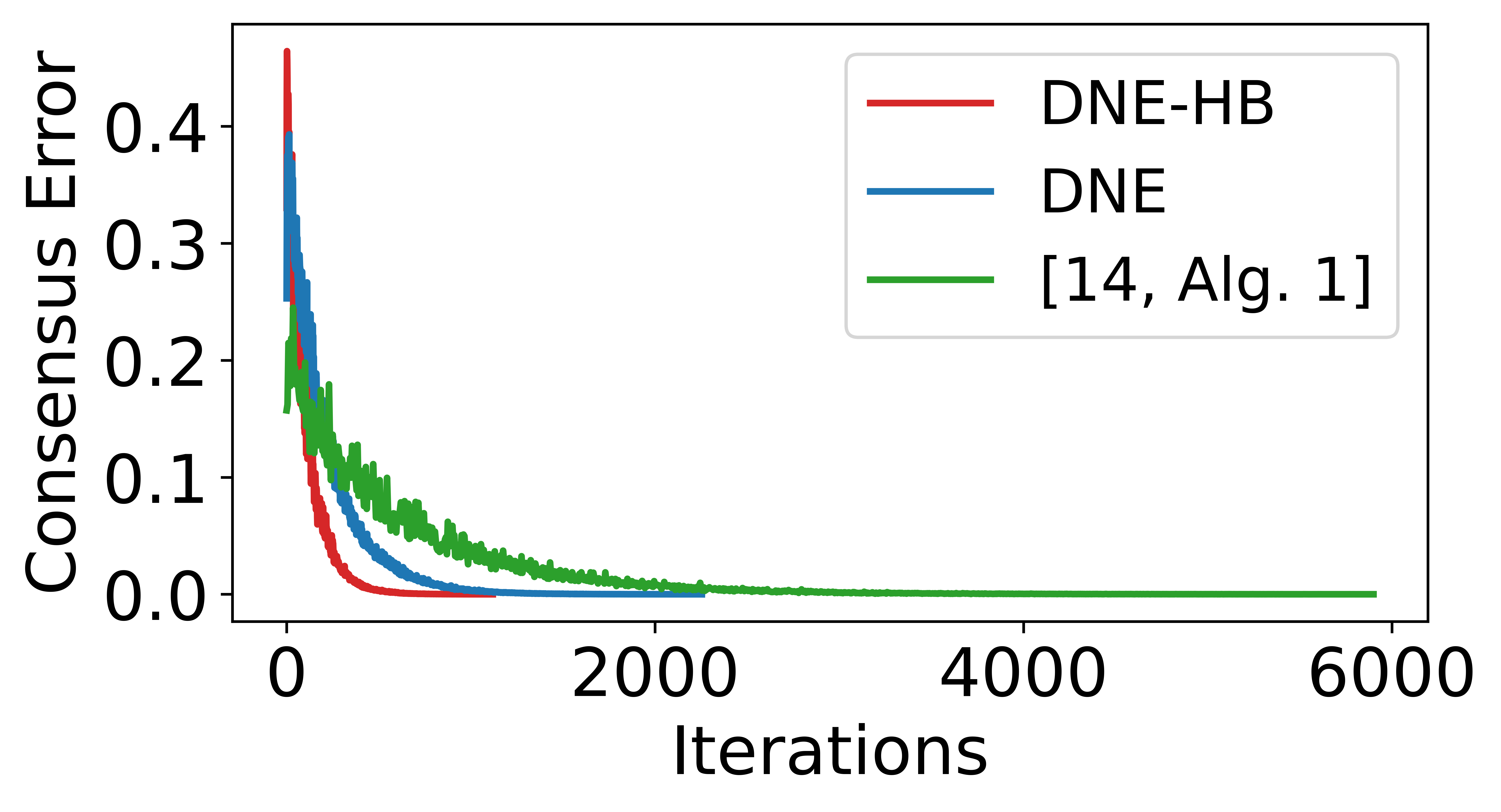
Refer to caption
Refer to caption
Fig. 1: Convergence behavior for one game instance.
Refer to caption
Fig. 2: Effects of varying the momentum parameter.

To demonstrate the accelerated convergence of DNE-HB, we compare it with existing agorithms including DNE (i.e. Algo. 1 of [15]) and Algo. 1 of [14]. We conduct 10001000 simulations with αi=0.01\alpha_{i}=0.01, βi=0.5\beta_{i}=0.5 and terminate the algorithms if the consensus error maxi∈[m],j∈[m],i≠j∥[𝐳k]i:−[𝐳k]j:∥∞\max_{i\in[m],j\in[m],i\neq j}\|[{\mathbf{z}}_{k}]_{i:}-[{\mathbf{z}}_{k}]_{j:}\|_{\infty} is less than 10−510^{-5} or the iteration limit of 10510^{5} is reached. Figure 1 shows the convergence for a game instance. Figure 2 illustrates the effect of momentum parameter on convergence rate. These results suggest that the algorithm converges faster with larger momentum parameter values satisfying the range in (32). Table I further compares the average performance of the algorithms over 10001000 simulations. Overall, the results demonstrate that the proposed algorithm with the heavy-ball acceleration significantly improves the convergence rate.

Stepsize Avg. # Iterations Avg. Running Time (s)
DNE DNE-HB DNE DNE-HB
αi=0.005\alpha_{i}=0.005 3667.523667.52 1826.441826.44 1.07031.0703 0.59840.5984
αi=0.01\alpha_{i}=0.01 2032.252032.25 1006.561006.56 0.67020.6702 0.35020.3502
TABLE I: Average performance over 10001000 simulations.

VI Conclusions and Future Work

This paper has proposed an accelerated distributed algorithm that incorporates heavy-ball acceleration to improve the performance of the gradient-based distributed NE-seeking algorithm for games over time-varying directed networks. A geometric convergence rate of the algorithm is shown with explicit bounds for the non-identical step-sizes and momentum parameters based on the properties of the cost functions and network structure. Our numerical results illustrate the effectiveness of the proposed method. In future, we will study its convergence for games with constrained action sets.

References

  • [1] W. Saad, Z. Han, H. V. Poor, and T. Basar, “Game-Theoretic Methods for the Smart Grid: An Overview of Microgrid Systems, Demand-Side Management, and Smart Grid Communications,” IEEE Signal Process. Mag., vol. 29, no. 5, pp. 86–105, 2012.
  • [2] D. T. A. Nguyen, J. Cheng, D. T. Nguyen, and A. Nedić, “CrowdCache: A Decentralized Game–Theoretic Framework for Mobile Edge Content Sharing,” arXiv preprint arXiv:2304.13246, 2023.
  • [3] P. Yi and L. Pavel, “An Operator Splitting Approach for Distributed Generalized Nash Equilibria Computation,” Automatica, vol. 102, pp. 111–121, 2019.
  • [4] G. Belgioioso and S. Grammatico, “Projected-Gradient Algorithms for Generalized Equilibrium Seeking in Aggregative Games are Preconditioned Forward-Backward Methods,” in 2018 European Control Conference (ECC), 2018, pp. 2188–2193.
  • [5] D. Gadjov and L. Pavel, “A Passivity-Based Approach to Nash Equilibrium Seeking Over Networks,” IEEE Trans. Autom. Control, vol. 64, no. 3, pp. 1077–1092, 2019.
  • [6] J. Koshal, A. Nedić, and U. V. Shanbhag, “Distributed Algorithms for Aggregative Games on Graphs,” Operations Research, vol. 64, no. 3, pp. 680–704, 2016.
  • [7] T. Tatarenko and A. Nedić, “Geometric Convergence of Distributed Gradient Play in Games with Unconstrained Action Sets,” IFAC-PapersOnLine, vol. 53, pp. 3367–3372, 01 2020.
  • [8] F. Salehisadaghiani, W. Shi, and L. Pavel, “Distributed Nash Equilibrium Seeking Under Partial-Decision Information via the Alternating Direction Method of Multipliers,” Automatica, vol. 103, pp. 27–35, 2019.
  • [9] T. Tatarenko, W. Shi, and A. Nedić, “Accelerated Gradient Play Algorithm for Distributed Nash Equilibrium Seeking,” in 2018 IEEE Conf. Decis. Control (CDC), 2018, pp. 3561–3566.
  • [10] ——, “Geometric Convergence of Gradient Play Algorithms for Distributed Nash Equilibrium Seeking,” IEEE Trans. Autom. Control, vol. 66, no. 11, pp. 5342–5353, 2021.
  • [11] G. Belgioioso, A. Nedić, and S. Grammatico, “Distributed Generalized Nash Equilibrium Seeking in Aggregative Games on Time-Varying Networks,” IEEE Trans. Autom. Control, vol. 66, no. 5, pp. 2061–2075, 2021.
  • [12] F. Salehisadaghiani and L. Pavel, “Nash Equilibrium Seeking with Non-doubly Stochastic Communication Weight Matrix,” EAI Endorsed Trans. Collaborative Computing, vol. 4, no. 13, pp. 3–15, 2019.
  • [13] M. Bianchi and S. Grammatico, “Fully Distributed Nash Equilibrium Seeking Over Time-Varying Communication Networks With Linear Convergence Rate,” IEEE Control Syst. Lett., vol. 5, no. 2, pp. 499–504, 2021.
  • [14] ——, “Nash Equilibrium Seeking under Partial-Decision Information Over Directed Communication Networks,” in 2020 59th IEEE Conf. Decis. Control (CDC), 2020, pp. 3555–3560.
  • [15] D. T. A. Nguyen, D. T. Nguyen, and A. Nedić, “Distributed Nash Equilibrium Seeking over Time-Varying Directed Communication Networks,” arXiv preprint arXiv:2201.02323, 2022.
  • [16] D. Gadjov and L. Pavel, “An Algorithm for Resilient Nash Equilibrium Seeking in the Partial Information Setting,” IEEE Transactions on Control of Network Systems, pp. 1–10, 2023.
  • [17] B. Polyak, Introduction to Optimization. New York : Optimization Software, Inc., 1987.
  • [18] D. T. A. Nguyen, D. T. Nguyen, and A. Nedić, “Accelerated AB/Push-Pull Methods for Distributed Optimization over Time-Varying Directed Networks,” arXiv preprint arXiv:2302.01214, 2023.
  • [19] C. Song, C. Wu, Z. Lv, F. Zhang, J. Li, and S. Yang, “Distributed Heavy-Ball Nash Equilibrium Seeking Algorithm in Aggregative Games,” in 39th Chinese Control Conference, 2020, pp. 5019–5024.
  • [20] X. Fang, G. Wen, J. Zhou, J. Lu, and G. Chen, “Distributed Nash Equilibrium Seeking for Aggregative Games With Directed Communication Graphs,” IEEE Trans. Circuits Syst. I: Regul. Pap., vol. 69, no. 8, pp. 3339–3352, 2022.
  • [21] G. Belgioioso and S. Grammatico, “Semi-Decentralized Generalized Nash Equilibrium Seeking in Monotone Aggregative Games,” IEEE Trans. Autom. Control, vol. 68, no. 1, pp. 140–155, 2023.
  • [22] M. Bianchi, G. Belgioioso, and S. Grammatico, “Fast Generalized Nash Equilibrium Seeking under partial-Decision Information,” Automatica, vol. 136, p. 110080, 2022.
  • [23] A. Nedić, D. T. A. Nguyen, and D. T. Nguyen, “AB/Push-Pull Method for Distributed Optimization in Time-Varying Directed Networks,” arXiv preprint arXiv:2209.06974, 2022.
  • [24] F. Facchinei and J.-S. Pang, Finite-Dimensional Variational Inequalities and Complementarity Problems. Springer Series in Operations Research and Financial Engineering, 2003.
  • [25] S. Pu, W. Shi, J. Xu, and A. Nedić, “Push–Pull Gradient Methods for Distributed Optimization in Networks,” IEEE Trans. Autom. Control, vol. 66, no. 1, pp. 1–16, 2021.
  • [26] G. Scutari, F. Facchinei, J.-S. Pang, and D. P. Palomar, “Real and Complex Monotone Communication Games,” IEEE Transactions on Information Theory, vol. 60, no. 7, pp. 4197–4231, 2014.