A Spatially Correlated Competing Risks Time-to-Event Model for Supercomputer GPU Failure Data

The data used in this paper is described in ?), which provide failure-time data for more than 30,000 GPUs that were in use during the service period of the Titan supercomputer, ranging from 2012 to 2019. We consider the OTB and DBE failure modes to obtain a more complete understanding of GPU reliability.

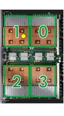
Inside the Titan supercomputer, there were 25 columns and 8 rows of cabinets, with 3 cages inside each cabinet, 8 slots in each cage, 4 nodes in each slot, and one GPU was installed on each node. Figure 1 shows the structure of the Titan supercomputer from ?). The yellow dots on the three sub-figures represent the GPU at column 17, row 4, cage 1, slot 3 and node 1. The GPU dataset contains the following information: the serial number of GPUs in Titan, the positions of GPUs inside cabinets (i.e., the cage, slot, and node information), the row and column locations of cabinets, the failure/service time of GPUs, and the GPU failure mode (i.e., DBE, OTB, or censored for GPUs that did not fail).

According to ?), GPUs that were first installed before 01 January 2016 were labeled as the old batch, and those that were installed after 01 January 2016 were labeled as the new batch. ?) indicated that the failure-time distributions of the old and new batches are different, because of different failure mechanisms. Thus, it would be misleading to pool the data for analysis. In addition, there were only a few new-batch GPUs that failed, and most locations had not observed any failures yet. Thus, there is not enough information in the data for spatial modeling of new-batch GPUs. Based on those considerations, we use the GPU data from the old batch for the modeling and analysis in this paper. As a summary, there are 1,127 OTB events, 3,093 DBE events, and 15,099 censored observations, and in total, there are 19,319 GPU in the old batch that are used in analysis.

Figure 2 shows barplots of discretized estimated probability mass function of OTB and DBE failures using Kaplan-Meier estimator. The barplots are built according to the method introduced in ?). From the barplot of DBE, we can clearly see a bimodal behavior of failure times, and the mode for the first DBE failure component nears the mode of OTB failure, which is around $3.5$ years. It is interesting to point out that the bimodal behavior of DBE failure times could indicate that there are two causes for DBE failures (i.e., one cause for early failures and another cause for later failures). Because DBE failures are memory errors and OTB failures are disconnects, it is possible that one of the causes for DBE failures is similar to the cause of OTB failures. We, however, do not have any explicit further information about the causes. Thus, we model the bimodal behavior using a mixture distribution with two components.

To visualize the spatial effects, Figure 3 shows the marginal OTB and DBE failure proportions at $200$ different cabinet locations ($25$ columns and $8$ rows). The marginal failure proportion on one location is the number of OTB or DBE failed GPUs on the location divided by the total number of GPUs on the location. It is clear that the marginal failure proportions at different locations are different, indicating the existence of spatial effects.

We group GPUs by different cabinet locations. Let $i$ be the location of a GPU cabinet, and $j$ be the index for a GPU inside one cabinet. There are $25$ columns and $8$ rows of cabinets for the overall system, so we have $i={1,2,\ldots,n}$, and there are $n=200$ locations. We have $j={1,2,\ldots,n_{i}}$, and $n_{i}$ is the total number of GPUs at location $i$. Note that $n_{i}$ can vary from location to location, and the sum of the $n_{i}$ values is equal to the total number of GPUs in the dataset. Let $T_{ijk}$ be the random variable of failure time for unit with cabinet location index $i$ and inside cabinet index $j$ having failure mode $k$. Let $t_{ij}$ be the observed failure time for failed (censored) unit with cabinet location index $i$ and inside cabinet index $j$. Let $\delta_{ijk}$ be the event-type indicator. That is, $\delta_{ijk}=1$ when unit $(i,j)$ failed because of failure mode $k$, and $k={1,2}$ for the two failure modes. Note that for a censored observation $\delta_{ij1}=\delta_{ij2}=0.$

Let $\boldsymbol{x}_{j}=(x_{j1},\ldots,x_{jp})^{\prime}$ be the covariate vector with inside cabinet index $j$. Because the cage, slot, and node positions are categorical with $3$ cage levels, $8$ slot levels, and $4$ node levels, respectively, we use dummy variable coding. In total, we have $p=12$ where $p$ is the total number of covariates. Let $\boldsymbol{z}_{i}=(r_{i},c_{i})^{\prime}$ be the row and column location index for units with location index $i$, where $r_{i}$ is the row index and $c_{i}$ is the column index. Here, $r_{i}$ can take values ${0,1,\ldots,7}$, and $c_{i}$ can take values ${0,1,\ldots,24}$. During the service period of the Titan supercomputer, some GPUs were swapped with GPUs from another location. For those GPUs, we follow the convention in ?) and use the location where the GPU spent the majority of its service time to determine the value of $c_{i}$ and $r_{i}$ for that unit. In summary, the time-to-event data are denoted by $\boldsymbol{t}=\{t_{ij},\delta_{ijk},\boldsymbol{z}_{i},\boldsymbol{x}_{j}\}$, $i=1,\ldots,n$, $j=1,\ldots,n_{i}$, and $k=1,2$.

We model the time to event $T_{ijk}$ using distributions from the log-location-scale family. In particular, we use a single log-location-scale distribution to describe the distribution of $T_{ij1}$ for OTB (failure mode 1). Because of the multimodal pattern of DBE failure (failure mode 2) seen in Figure 2, we model failure mode 2 with a mixture of two different log-location-scale distributions. Specifically, for OTB failures (failure mode $1$, $k=1$), the probability density function (pdf) and cumulative distribution function (cdf) can be represented as,

where $\mu_{ijk}$ and $\xi_{k}$ are the location and scale parameters for the location-scale distribution corresponding to observation $i$ with inside cabinet index $j$ and failure mode $k$, respectively. We consider two widely used distributions from the log-location-scale family, namely the Weibull distribution and lognormal distributions (e.g., Chapter 4 in [Meeker et al. (2022]). In (1), $\phi(z)$ and $\Phi(z)$ are the standard pdf and cdf from the location-scale distribution, which can be the smallest extreme value (SEV) distribution or the normal distribution in the paper. Also, $w_{ik}$ is a spatial random effect that will be discussed later.

We model the distribution of DBE failures (failure mode $2$, $k=2$) with a mixture distribution and the pdf is

where $\mu_{ijk1}$ and $\mu_{ijk2}$ are the two location parameters, and $\xi_{k1}$ and $\xi_{k2}$ are the two scale parameters of the corresponding location-scale distributions for the mixture components. We use $\lambda$ to represent the mixture proportion. One commonly known issue of mixture modeling is the label switching problem, which makes the model not identifiable. A simple way to solve this problem is to add constraints on the parameters to make the likelihood asymmetric with respect to the two mixed distributions [Jasra et al. (2005]. In particular, for the mixture distribution in (2), we use the restriction $\mu_{ijk1}<\mu_{ijk2}$ to avoid identifiability problems in estimation.

In summary, the location parameters are modeled as follows,

Under failure mode $k$, $\boldsymbol{\beta}_{k}$ contains the corresponding coefficients for $\boldsymbol{x}_{j}$, $w_{ik}$ corresponds to the location random effect at cabinet location $\boldsymbol{z}_{i}$, and $\eta$ represents the difference between two components of the mixture distribution. In (3), $\mu_{1}$ is the baseline of the $\mu_{ij1}$ parameter for event time when $w_{i1}=0$. In (4) and (5), $\mu_{2}$ is the baseline for the first mixture component when $w_{i2}=0$ and $\mu_{2}+\eta$ is the baseline for the second mixture component when $w_{i2}=0$. By setting $\eta>0$, we can avoid the identifiability problem. Note that the pdf of the two failure modes can be separated by conditioning on the spatial random effects.

We now discuss the modeling of spatial random effects. Let $\boldsymbol{w}_{k}=(w_{1k},\ldots,w_{nk})^{\prime},k=1,2$ and $\boldsymbol{w}=(\boldsymbol{w}_{1}^{\prime},\boldsymbol{w}_{2}^{\prime})^{\prime}$. We model $\boldsymbol{w}$ by using a multivariate normal distribution $\textrm{MVN}(\boldsymbol{0},\Sigma_{\boldsymbol{w}})$, and the covariance matrix $\Sigma_{\boldsymbol{w}}$ is $\Sigma_{\boldsymbol{w}}=\Sigma_{f}\otimes\Omega,$ where $\otimes$ is the Kronecker product. The covariance matrix of $(w_{i1},w_{i2})^{\prime},i=1,\ldots,n$, is

where $\sigma_{1}^{2}$ and $\sigma_{2}^{2}$ are variances for $w_{i1}$ and $w_{i2}$, respectively, and $\rho_{12}$ is the correlation between $w_{i1}$ and $w_{i2}$, which is used to model the correlation between the two failure modes. The spatial correlation matrix is,

with parameters $0<\kappa\leq 2$ and $\nu>0$, and $d_{sl}$ is the distance between cabinet locations. We consider three commonly used spatial correlation functions here, which are the Gaussian, exponential, and power exponential correlation functions [Sherman (2010]. These three different correlation functions have different $\kappa$ values in (6). The Gaussian correlation function has fixed $\kappa=2$, the exponential correlation function has fixed $\kappa=1$, and the power exponential correlation function has a power $0<\kappa\leq 2$ that is not fixed.

Our method of quantifying the distances between GPU cabinets requires some discussion. We want to point out that here the column index of the cabinet is labeled according to the connectivity of the cabinets but not the physical locations of the cabinets. In Titan, column 0 (under the current labeling) is connected to column 1 (under the current labeling), column 1 is connected to column 2, and so on. Then column 24 is connected back to column 0. Figure 4 visualizes the spatial connectivity, as indexed by row and column. Each intersecting point represents a cabinet. Our preliminary analysis showed that relabeling the column index using this connectivity is necessary. Failure proportions of different rows and columns without relabeled column indices (i.e., using the original physical location labels) are shown in Appendix B. The figures show that the pattern of failure proportions is more clearly related to the column index based on connectivity. For the row index, we use the original row value to indicate the physical location.

To compute the distance between cabinet locations $d_{sl}$, we take into account the spatial connectivity of the columns of cabinets and the physical location of the rows of cabinets. The distance is defined as

because column 24 is connected back to column 0. Figure 4 provides a visualization of calculating distance between location $(r_{1},c_{23})$ to $(r_{3},c_{1})$, and $(r_{6},c_{2})$ to $(r_{1},c_{4})$. Using (7), the distance between column 0 and column 24 is 1. Thus, the column labels form a circle and the rows and columns together form a cylinder. Note that we also normalize $(r_{s}-r_{l})$ and $\min\{|c_{s}-c_{l}|,25-|c_{s}-c_{l}|\}$ to range $[0,1]$ in calculating $d_{sl}$ to make the connectivity and physical distance have an equal contribution in the distance calculation. The largest distance is $d_{sl}=\sqrt{2}$. As noted by ?), distances defined on a sphere can result in a non-positive definite correlation matrix. Our distance is different from that used in existing work because it is like a cylinder. Thus, some special attention is needed to assure positive definiteness. We describe the accommodations in Section 3.3 as part of the modeling process.

Let $\boldsymbol{\theta}_{\boldsymbol{t}}$ be the unknown parameters corresponding to the time-to-event distribution of $T_{ijk}$ and let $\boldsymbol{\theta}_{\boldsymbol{w}}$ be the unknown parameters for the distribution of random effects. Specifically, $\boldsymbol{\theta}_{\boldsymbol{t}}=(\mu_{1},\mu_{2},\boldsymbol{\beta}_{1}^{\prime},\boldsymbol{\beta}_{2}^{\prime},\xi_{1},\xi_{21},\xi_{22},\lambda,\eta)^{\prime}$ and $\boldsymbol{\theta}_{\boldsymbol{w}}=(\sigma_{1},\sigma_{2},\rho_{12},\nu,\kappa)^{\prime}$. The likelihood, conditional on fixed values of the spatial random effects $\boldsymbol{w}$ is,

The joint density for $\boldsymbol{w}$ is,

Then, the likelihood for $\boldsymbol{\theta}=(\boldsymbol{\theta}_{\boldsymbol{t}}^{\prime},\boldsymbol{\theta}_{\boldsymbol{w}}^{\prime})^{\prime}$ is,

For $\boldsymbol{\theta}_{\boldsymbol{t}}$, we choose flat priors for the unrestricted parameters $\mu_{k}$ and $\boldsymbol{\beta}_{k}$, and uniform priors for the restricted parameters $\lambda$ and $\eta$. Because the domain of the $\xi_{k}$’s is $(0,\infty)$, we use the noninformative prior for $\xi_{k}$’s. In particular, the priors are specified as,

For $\boldsymbol{\theta}_{\boldsymbol{w}}$, we use noninformative priors for most parameters, and use an inverse Gamma (IG) prior for $\nu$, and a Beta prior for $\kappa/2$. Specifically,

We can choose the values of $a,b,c$, and $d$ for specific priors of $\nu$ and $\kappa$. In the simulation study and the GPU data application, we set $c=d=1$ so that $\kappa$ has a proper flat prior. It is common to use the IG distribution as a prior distribution for $\nu$, and we set $a=5$ and $b=1$ to penalize large values of $\nu$ to guarantee the positive definiteness of the $\Omega$ matrix.

Essentially the correlation matrix $\Omega$ is a function of $\nu$ and $\kappa$, given the distance matrix $(d_{sl})$. Thus, we can compute the smallest eigenvalue of $\Omega$ given $\nu$ and $\kappa$. Figure 5 shows the heatmap and contour lines of the smallest eigenvalue for $\Omega$ as a function of $\nu$ and $\kappa$. The darker the color, the smaller the smallest eigenvalue. The figure indicates that when $\nu$ is large, it is possible that the correlation matrix is not positive definite. Therefore we give low prior density to large $\nu$ values. The probability that $\nu$ is less than or equal to $0.5$ is about $0.95$ under its prior distribution. The black dots represent $500$ draws of $\kappa$ and $\nu$ based on the joint prior distribution. Although the correlation function of the spatial random effects decreases rapidly for values of $\nu$ less than $0.5$ and values of $\kappa$ close to $2$, the power exponential correlation function is still flexible, because both $\nu$ and $\kappa$ are not fixed. That is, different combinations of $\nu$ and $\kappa$ values can achieve correlation functions that are similar to each other.

Based on the likelihood and the prior specification, the joint posterior distribution is

where $f(\boldsymbol{\theta}_{\boldsymbol{t}})$ and $f(\boldsymbol{\theta}_{\boldsymbol{w}})$ are the joint prior distribution for $\boldsymbol{\theta}_{\boldsymbol{t}}$ and $\boldsymbol{\theta}_{\boldsymbol{w}}$, respectively. Although we used improper priors for $\mu_{k}$, $\boldsymbol{\beta}_{k}$, $\xi_{k}$, $\sigma_{1}$ and $\sigma_{2}$, the posterior is proper. That is,

For the $\int f(\boldsymbol{w}|\boldsymbol{\theta}_{\boldsymbol{w}})f(\boldsymbol{\theta}_{\boldsymbol{w}})d\boldsymbol{\theta}_{\boldsymbol{w}}$ part, it is commonly known that the improper priors for $\sigma_{1}$ and $\sigma_{2}$ lead to proper posterior with more than two random effects. For the integral $\int L(\boldsymbol{\theta}_{\boldsymbol{t}}|\boldsymbol{t},\boldsymbol{w})f(\boldsymbol{\theta}_{\boldsymbol{t}})d\boldsymbol{\theta}_{\boldsymbol{t}}$, with a sufficient amount of data, the improper priors lead to a proper posterior for a Weibull or a lognormal time-to-event distribution. For the Weibull distribution, ?) proved that, for a single distribution, the posterior is proper when there are at least two failures in the data. We extend the result for a regression model by using a different parametrization and using an improper noninformative prior for the regression coefficient $\boldsymbol{\beta}_{k}$. The proof is in Appendix A. For the lognormal distribution, the posterior is proper when the number of failures for each failure mode is larger than $(p+3)/2$, and $p$ is the dimension of the covariates. The proof is similar to that the normal regression model with flat priors on covariates and variances lead to proper posteriors.

Because the likelihood $L(\boldsymbol{\theta}_{\boldsymbol{t}}|\boldsymbol{t},\boldsymbol{w})$ for the two failure modes in (8) can be factored into likelihoods for the two failure modes, the posterior $L(\boldsymbol{\theta}_{\boldsymbol{t}}|\boldsymbol{t},\boldsymbol{w})f(\boldsymbol{\theta}_{\boldsymbol{t}})$, for the two failure modes can be separated, and the integral involved in showing the properness of the posterior can be done in parts. Thus, it is sufficient to prove that the posterior for one failure mode is proper. Also, because we use a proper prior on the mixture probability $\lambda$, we focus on the situation where there is only one failure mode in the failure-time distribution.

Based on the above discussion, for notational simplicity in the statement of the result and its proof, we drop the index $k$ and resort the data by one index $i$. That is, we use $t_{i}$ to denote the event time, $\delta_{i}$ for the event-type indicator, and $w_{i}$ for the corresponding random effect, $\mu$ for the log-location parameter, $\xi$ for the log-scale parameter, and $\boldsymbol{\beta}$ for the regression coefficients. Let $\boldsymbol{\Psi}=(\mu,\boldsymbol{\beta}^{\prime},\xi)^{{}^{\prime}}$. Suppose that $\sum_{i}\delta_{i}=m$ is the number of observed failures, and $p$ is the length of $\boldsymbol{\beta}$. We summarize the result in the following proposition.

The proof of Proposition 1 is given Appendix A. Proposition 1 provides part of the theoretical basis for the inference using the posterior distribution.

In the spatially correlated failure times application, we jointly sample $f(\boldsymbol{\theta},\boldsymbol{w}|\boldsymbol{t})$ using Markov chain Monte Carlo (MCMC). We transform all parameters to have a range $(-\infty,\infty)$. We have seen that doing this improves the Stan NUTS sampler. Let $\widetilde{\boldsymbol{\theta}}$ be the transformed unrestricted parameters, then,

Also, we transform the random effect matrix to avoid linear dependency on $\mu_{k}$. Let $A=n^{-1}(I_{n}-J_{n})$ and $A\boldsymbol{w}_{k}$ is the transformed spatial random vector for $k=1,2$. We take the first $n-1$ elements of $A\boldsymbol{w}_{k}$ as the spatial random effect parameters for failure mode $k$, and only use these $n-1$ elements in MCMC sampling. To make the MCMC sampling more numerically stable, we also constrain the range of $\rho_{12}$ to be between $-0.95$ and $0.95$.

After we obtain the draws from posterior distribution, we use the posterior means to obtain point estimates. Also, $95\%$ equal tail credible intervals (CI) are computed from the 0.025 and 0.975 empirical quantiles of the marginal posterior draws for quantities of interest.

We study the influence of two factors: the number of units $N$, and the number of spatial locations $d\times d$, on model estimation. We carefully choose value of true parameters to mimic the real GPU dataset. Because the model used for the GPU data is quite sophisticated, to simplify the setting and reduce the computing time, we use one inside cabinet position covariate. In particular, we use the cage factor with three different levels; thus the column rank of the design matrix is $p=2$, and $p$ is the number of covariates. To simplify the setting, we use the same number of rows and columns (i.e., both of number of columns and rows are $d$) for the location setting. We chose $N$ to be 5,000, 7,000, and 10,000, and we chose $d$ to be 5, 7, and 10. In practice, we learned that when the number of failed GPUs is small (i.e., zero failures or one failure) on multiple locations, the posterior samples of the random effects variances stay at the same value in some MCMC chains. Therefore, in simulating the data, we require the proportion of locations that have at least 1 failure is greater than $5\%$, and the proportion of locations have at least 2 failures is greater than $10\%$. We generate the simulation dataset 300 times under each factor-level combination. The value of true parameters are shown in Table 1.

Under each factor-level combination, for each of the $N$ units, we first sample from Binom($3$, $0.5$), and then remove the last column of the $N\times 3$ matrix to obtain the model matrix. For the cabinet location index, we uniformly sample row and column index from $1$ to $d$. We then sample failure times for failure mode type 1 and failure mode type 2 of each unit from two independent Weibull distributions based on the covariates and random effects. Using a simplified setting, we generate beginning date for each GPU from a uniform distribution with the lower bound as 01 January 2012, and the upper bound as 01 January 2018. We set the end date as 01 January 2019. Units that have not failed before 01 January 2019 is categorized as censored. Figure 6 shows the failure proportions of failure mode types $1$ and $2$ from one dataset generated using $7\times 7$ spatial random effects and 7,000 units.

For each factor-level combination and for each simulation trial, we run $3$ chains with 2,000 draws after warmup per chain, providing 6,000 draws in total. We use random starting values picked by Stan. We check the convergence using Rhat introduced in ?) and use cutoff $1.1$ to decide whether a chain converged or not. We noticed that there are some MCMC chains in which the samples of random effect variances were not moving. However, the proportion of such chains is relatively small (i.e., less than 1%) for each factor-level combination. For those chains, we use the same data and run the MCMC again with different starting values picked by Stan. If the chains still do not converge, we exclude the dataset and generate a new dataset. Among all 27,000 simulation runs, only four such datasets were excluded.

Figure 7 shows the RRMSE for parameter estimators for $\boldsymbol{\theta}$. More results about the relative bias, estimated standard deviation, coverage probability, and mean CI length are in Appendix C. The RRMSEs are small for all the situations. For most parameters, the RRMSE decreases as the number of units increases. There is no evident trend in relative bias or standard deviation as $N$ in contrast to the observed trend of RRMSE. In addition, when the number of locations increases from $5\times 5$ to $7\times 7$, the relative bias of both $\nu$ and $\kappa$ decreases for all three levels of $N$. The coverage probability of CI is close to the nominal $0.95$ level for all the cases. The mean length of CIs decreases as the number of units increases for all parameters. When the number of locations increases, the mean length of CIs for $\nu$ and $\kappa$ decreases.

In this section, we fit the models proposed in Section 3.1 to the GPU data. We ran $4$ chains, and we generated 2,000 draws from each chain after an initial 6,000 draws. Because the regular residuals are not defined for a mixture distribution time-to-event model, we define our residuals as $r_{ijk}=-\log(1-\widehat{F}(t_{ij}|w_{ik})),$ where $\widehat{F}(t_{ij}|w_{ik})$ is obtained by substituting the estimates of parameters $\boldsymbol{\theta}$. Because the residuals should have WEIB$(0,1)$ distribution (if the fitted model is correctly specified), we assess their distributions by using Weibull probability plots.

We first fit the model with a Weibull time-to-event distribution and a power exponential spatial correlation function. Figure 8 shows the result for the estimated residuals of the model. The red lines are WEIB$(0,1)$ distributions and the black dots are estimated points. Except for the three data points in Figure 8(a), the residuals agree well with the $\textrm{WEIB}(0,1)$ reference line, suggesting that the model is fitting reasonably well.

As a quick overview of estimation results, Figure 9 shows the estimates and $95\%$ CIs for the inside cabin locations. Table 2 shows the estimate and $95\%$ credible interval for all of the other parameters. Figure 10 shows the estimated random effects at different cabin locations.

Because the Weibull and lognormal are two commonly used parametric distributions for modeling time-to-event data, we also compare the model performance for these two distributions. In addition, we consider five correlation models: the power exponential (PEXP), the exponential (EXP), and the Gaussian (GAU) correlation functions, the AFT models with no spatial correlated random effects (AFT INDEP), and the AFT models with no random effects. All the models we consider are listed in Table 3.

We compare all the models using the leave-one-out cross-validation information criterion (LOOIC) in ?). Table 3 shows the LOOIC for all the models. The comparison indicates that the Weibull PEXP model is the best one in terms of LOOIC. The comparison also shows that adding spatial random effects to the model is important. The estimates and CIs of the parameters for those models are given in Appendix F.

There are other estimation methods for fitting a time-to-event model with random effects. When using a Bayesian model, the integrated nested Laplace approximation (INLA) [Rue et al. (2009] can be used for approximate Bayesian inference. For frequentist inference, the EM algorithm can be used to obtain maximum likelihood estimators. However, INLA can not be directly implemented in our case because of the mixture distribution for the DBE failure mode. Therefore, we compare our Bayesian results (i.e., the Weibull PEXP model with the best LOOIC) with EM algorithm results. Details about the formulas and implementation of EM algorithm are in Appendix D. The EM estimates are also available in Appendix D. All EM estimates for parameters are within the CIs from the Bayesian method, indicating good agreement from different methods. However, we do notice that the EM algorithm is much slower due to the use of MCMC in the E step for each iteration.

In this section, we show the estimation results for the Weibull PEXP model. Figure 10 shows the estimated random effects at different cabinet locations, suggesting that the mode of failure times varies among cabinet locations. A larger random effect indicates that the GPUs at those locations tend to have longer lifetimes. From Figure 10, we can see that the column marginals transition from positive values, to negative values and then to positive values, by using the labels from the logical connection. We also can see that the row marginals transition from negative values to positive values (shorter lifetimes to longer lifetimes) from row 0 to row 7, which may be caused by physical cooling heterogeneity from row 0 to row 7. As indicated in Figure 1(a), heat dissipation near a wall (near row 0) may not be as good as in an open space (near row 7). Figure 9 shows the estimates and $95\%$ CIs for the inside cabinet positions. Table 2 shows the estimate and $95\%$ CI for all other parameters. The baseline levels for categorical variables cage, slot, and node are cage $2$, slot $7$, and node $3$. The estimated coefficients in Figure 9 shows the difference on the log scale of the mode of the failure times between current cage, slot, node levels and the baseline levels, holding other parameters fixed. The positive estimates in Figure 9(a) indicate that the failure time for GPUs inside cage $0$ and cage $1$ tend to be longer than those for the GPUs inside cage $2$. The difference between cage $0$ and cage $1$ is also significant. The cage effect is likely due to differences in the temperature in the supercomputer. The temperature around cages at the bottom floors of the cabinets is lower than the cages at higher floors of the cabinets, because of the airflow inside the supercomputer. In addition, the influence of the positions of cages within cabinets is stronger for OTB failures than for DBE failures, which shows that the OTB failure mechanism is more sensitive to temperature.

On the other hand, the negative estimate in Figure 9(c) shows that GPUs on node $3$ have the longest failure times when compared with GPUs on nodes 0–2. The difference between nodes 0–1 and nodes 2–3 may also be caused by temperature differences similar to the differences among different positions of cage. This is because nodes 0–1 are at a lower vertical level than nodes 2–3, as shown in Figure 1(c). Slot position influence is relatively weak compared with cage and node position influence, and the influence of slot on the OTB and DBE failure-time distributions is similar. An explanation for this is that the cooling condition is relatively uniform for slots across the same cage (see Figure 1(b) which depicts the within cabinet layout).

The estimates of parameters related to the spatial random effects suggest that the row-column cabinet locations also have an effect on the failure-time distributions. Table 2 shows that the posterior means of $\sigma_{1}$ and $\sigma_{2}$ are $0.13$ and $0.11$, suggesting that the variation of random effects exists. The estimate of $\rho_{12}$ and its corresponding CI in Table 2 provide evidence of strong positive correlations between OTB spatial random effects and DBE spatial random effects. Figure 11 shows the curve of the spatial correlation function. The black line is the posterior mean, and the two blue lines are lower and upper endpoints of the CI of the correlation function. The correlation decays rapidly, and the value at the largest distance ($\sqrt{2}$) in the dataset is around $0.002$.

We can also estimate the marginal posterior correlation between the OTB failure time and the DBE failure times at different cabinet locations and inside cabinet positions by integrating out the random effects. The formulas and calculation steps are given in Appendix G. The correlation between $T_{ij1}$ and $T_{ij2}$ depends on the value of the covariates $\boldsymbol{x}_{j}$. At inside cabinet position cage 2, slot 7, and node 1, the estimated correlation between $T_{ij1}$ and $T_{ij2}$ is 0.24. At inside cabinet position cage 0, slot 7 and node 3, the estimated correlation is 0.21. Also, for a fixed index $j$ (i.e., fixed inside cabinet position), we compute the marginal correlation between $T_{ijk}$ and $T_{i^{\ast}jk}$, $i\neq i^{\ast}$. Figure 12 shows the correlation curve for $T_{ijk}$ and $T_{i^{\ast}jk}$. To show the trend of the correlation curve, the $x$-axis is the distance value. The small fluctuation when distance is large comes from estimation error.

References

- Carroll et al. (2019 Carroll, R., A. B. Lawson, and S. Zhao (2019). Temporally dependent accelerated failure time model for capturing the impact of events that alter survival in disease mapping. Biostatistics 20, 666–680.
- Chang et al. (2013 Chang, H. H., B. J. Reich, and M. L. Miranda (2013). A spatial time-to-event approach for estimating associations between air pollution and preterm birth. Journal of the Royal Statistical Society: Series C (Applied Statistics) 62, 167–179.
- Di et al. (2017 Di, S., R. Gupta, M. Snir, E. Pershey, and F. Cappello (2017). Logaider: A tool for mining potential correlations of HPC log events. In 2017 17th IEEE/ACM International Symposium on Cluster, Cloud and Grid Computing (CCGRID), pp. 442–451. IEEE.
- Geng and Hu (2022 Geng, L. and G. Hu (2022). Bayesian spatial homogeneity pursuit for survival data with an application to the SEER respiratory cancer data. Biometrics 78, 536–547.
- Gneiting (2013 Gneiting, T. (2013). Strictly and non-strictly positive definite functions on spheres. Bernoulli 19, 1327–1349.
- Gupta et al. (2015 Gupta, S., D. Tiwari, C. Jantzi, J. Rogers, and D. Maxwell (2015). Understanding and exploiting spatial properties of system failures on extreme-scale HPC systems. In 2015 45th Annual IEEE/IFIP International Conference on Dependable Systems and Networks, pp. 37–44. IEEE.
- Henderson et al. (2002 Henderson, R., S. Shimakura, and D. Gorst (2002). Modeling spatial variation in Leukemia survival data. Journal of the American Statistical Association 97, 965–972.
- Hennerfeind et al. (2006 Hennerfeind, A., A. Brezger, and L. Fahrmeir (2006). Geoadditive survival models. Journal of the American Statistical Association 101, 1065–1075.
- Hesam et al. (2018 Hesam, S., M. Mahmoudi, A. R. Foroushani, M. Yaseri, and M. A. Mansournia (2018). A cause-specific hazard spatial frailty model for competing risks data. Spatial Statistics 26, 101–124.
- Huzurbazar (2005 Huzurbazar, A. V. (2005). A censored data histogram. Communications in Statistics: Simulation and Computation 34, 113–120.
- Jasra et al. (2005 Jasra, A., C. C. Holmes, and D. A. Stehens (2005). Markov chain Monte Carlo methods and the label switching problem in Bayesian mixture modeling. Statistical Science 20, 50–67.
- Li et al. (2015 Li, J., Y. Hong, R. Thapa, and H. E. Burkhart (2015). Survival analysis of loblolly pine trees with spatially correlated random effects. Journal of the American Statistical Association 110, 486–502.
- Li and Lin (2006 Li, Y. and X. Lin (2006). Semiparametric normal transformation models for spatially correlated survival data. Journal of the American Statistical Association 101, 591–603.
- Li and Ryan (2002 Li, Y. and L. Ryan (2002). Modeling spatial survival data using semiparametric frailty models. Biometrics 58, 287–297.
- Meeker et al. (2022 Meeker, W. Q., L. A. Escobar, and F. G. Pascual (2022). Statistical Methods for Reliability Data (Second ed.). John Wiley & Sons.
- Meuer et al. (2020 Meuer, H., E. Strohmaier, J. Dongarra, H. Simon, and H. Simon (2020). Top 500 list of supercomputer sites. [Online]. Available: https://www.top500.org/.
- Młynarczyk et al. (2021 Młynarczyk, D., C. Armero, V. Gómez-Rubio, and P. Puig (2021). Bayesian analysis of population health data. Mathematics 9, 577.
- Momenyan and Poorolajal (2020 Momenyan, S. and J. Poorolajal (2020). Modeling of spatio-temporally clustered survival HIV/AIDS data in the presence of competing risks setting. Spatial Statistics 38, 100460.
- Motarjem et al. (2019 Motarjem, K., M. Mohammadzadeh, and A. Abyar (2019). Bayesian analysis of spatial survival model with non-Gaussian random effect. Journal of Mathematical Sciences 237, 692–701.
- Nie et al. (2018 Nie, B., J. Xue, S. Gupta, T. Patel, C. Engelmann, E. Smirni, and D. Tiwari (2018). Machine learning models for GPU error prediction in a large scale HPC system. In 2018 48th Annual IEEE/IFIP International Conference on Dependable Systems and Networks (DSN), pp. 95–106. IEEE.
- Onicescu et al. (2018 Onicescu, G., A. B. Lawson, J. Zhang, M. Gebregziabher, K. Wallace, and J. M. Eberth (2018). Spatially explicit survival modeling for small area cancer data. Journal of Applied Statistics 45, 568–585.
- Ostrouchov et al. (2020 Ostrouchov, G., D. Maxwell, R. A. Ashraf, C. Engelmann, M. Shankar, and J. H. Rogers (2020). GPU lifetimes on Titan supercomputer: Survival analysis and reliability. In SC20: International Conference for High Performance Computing, Networking, Storage and Analysis, pp. 1–14. IEEE.
- Pan et al. (2014 Pan, C., B. Cai, L. Wang, and X. Lin (2014). Bayesian semiparametric model for spatially correlated interval-censored survival data. Computational Statistics & Data Analysis 74, 198–208.
- Ramos et al. (2020 Ramos, E., P. L. Ramos, and F. Louzada (2020). Posterior properties of the Weibull distribution for censored data. Statistics & Probability Letters 166, 108873.
- Rue et al. (2009 Rue, H., S. Martino, and N. Chopin (2009). Approximate Bayesian inference for latent Gaussian models by using integrated nested Laplace approximations. Journal of the Royal Statistical Society: Series B (Statistical Methodology) 71, 319–392.
- Sherman (2010 Sherman, M. (2010). Spatial Statistics and Spatio-Temporal Data: Covariance Functions and Directional Properties. John Wiley & Sons.
- Tiwari et al. (2015 Tiwari, D., S. Gupta, G. Gallarno, J. Rogers, and D. Maxwell (2015). Reliability lessons learned from GPU experience with the Titan supercomputer at Oak Ridge leadership computing facility. In SC’15: Proceedings of the International Conference for High Performance Computing, Networking, Storage and Analysis, pp. 1–12. IEEE.
- Vehtari et al. (2017 Vehtari, A., A. Gelman, and J. Gabry (2017). Practical Bayesian model evaluation using leave-one-out cross-validation and WAIC. Statistics and Computing 27, 1413–1432.
- Vehtari et al. (2021 Vehtari, A., A. Gelman, D. Simpson, B. Carpenter, and P.-C. Bürkner (2021). Rank-normalization, folding, and localization: An improved for assessing convergence of MCMC (with discussion). Bayesian Analysis 16, 667–718.
- Wang et al. (2017 Wang, G., L. Zhang, and W. Xu (2017). What can we learn from four years of data center hardware failures? In 2017 47th Annual IEEE/IFIP International Conference on Dependable Systems and Networks (DSN), pp. 25–36. IEEE.
- Wang et al. (2016 Wang, S., J. Zhang, and A. B. Lawson (2016). A Bayesian normal mixture accelerated failure time spatial model and its application to prostate cancer. Statistical Methods in Medical Research 25, 793–806.
- Zhou and Hanson (2018 Zhou, H. and T. Hanson (2018). A unified framework for fitting Bayesian semiparametric models to arbitrarily censored survival data, including spatially referenced data. Journal of the American Statistical Association 113, 571–581.