Kernel based quantum machine learning at record rate:
Many-body distribution functionals as compact representations

We begin the discussion of our local representation using distribution functions over the internal coordinates which can be constructed using the atomic coordinates.

An analytical and continuous distribution over the pair-wise internal coordinate defined as the inter-atomic distances (pair correlation function), is easily built using Gaussian probability density functions (PDFs) centered at each inter-atomic distance with respect to an atom $i$:

$\displaystyle\rho_{i}(r,R_{ij})=\frac{1}{\sqrt{2\pi\sigma_{r}^{2}}}\sum_{j\neq i}^{M}Z_{j}\exp{\left(-{\frac{(r-R_{ij})^{2}}{\sigma_{r}}}\right)}$

(1)

where $\rho_{i}(r,R_{ij})$ is the normalized distribution with atom $i$ as the origin, $\sigma_{r}$ is the Gaussian length-scale (or variance) parameter, $M$ denotes the total number of atoms in the system (or within a radial cutoff if employed), $R_{ij}$ denotes the inter-atomic distance between atoms $i$ and $j$ and $Z_{j}$ is the nuclear charge. Scaling by nuclear charges defines elemental identities, but could also be done in other ways e.g. having different length-scale parameters $\sigma_{r}$ for each unique chemical element, or multiple dimensions such as period and group specifications ⁴³. In a similar fashion, a continuous distribution (triplet correlation function) over the 3-body internal coordinate, inter-atomic angles $\theta$, is defined as:

	$\displaystyle\rho_{i}(\theta,\theta_{jik})=\frac{1}{\sqrt{2\pi\sigma_{\theta}^{2}}}\sum_{j\neq i}^{M}\sum_{k\neq j}^{M}Z_{j}Z_{k}~\exp{\left(-\frac{(\theta-\theta_{jik})^{2}}{\sigma_{\theta}}\right)},$
	$\displaystyle\theta_{jik}=\cos^{-1}\frac{(\mathbf{R}_{i}-\mathbf{R}_{j})^{T}(\mathbf{R}_{i}-\mathbf{R}_{j})}{R_{ij}^{2}}$		(2)

where $\theta_{jik}$ is the inter-atomic angle centered on atom $i$. This can be generalized to define a continuous distribution, or correlation function, over any $m$-body internal coordinate $\tau$.
Such analytical distribution functions of the internal coordinates have been used as descriptors of atomic environments in Atom Centered Symmetry Functions^{20; 6} (ACSF), their weighted variants wACSFs²³ and other similar methods. Instead of using these distribution functions as atomic descriptors, we define the MBDF representation as functionals of these $m$-body distributions which leads to a more compact descriptor and allows inclusion of higher order terms with minimal change in size (a single scalar for each $m$-body term). With the 2- and 3-body distributions defined above, each atom can then be represented by the two zeroth-order functionals:

$\displaystyle F_{0}^{(2)}[i]=\int_{0}^{r_{c}}dr~g_{0}(r,R_{ij})~\rho_{i}(r,R_{ij})$

(3)

$\displaystyle F_{0}^{(3)}[i]=\int_{0}^{\pi}d\theta~g_{0}(\theta,R_{ij},R_{jk},R_{ik})~\rho_{i}(\theta,\theta_{jik})$

(4)

where $r_{c}$ denotes the radial cut-off distance, and $g_{0}(r,R_{ij})$ and $g_{0}(\theta,R_{ij},R_{jk},R_{kj})$ denote 2- and 3-body weighting functions. Note that when the weighting functions $g_{0}(r,R_{ij})$ and $g_{0}(\theta,R_{ij},R_{jk},R_{kj})$ correspond to suitable 2 and 3-body potentials, the functionals $F_{0}^{(2)}$, $F_{0}^{(3)}$ become the average of the corresponding 2, 3-body inter-atomic interactions weighted by the pair and triplet correlation functions $\rho_{i}(r,R_{ij})$, $\rho_{i}(\theta,\theta_{jik})$, respectively. These functionals then form a coarse approximation to the average 2, 3-body interactions experienced by a chemical species. Furthermore, we exploit the advantage of using the infinitely differentiable Gaussian PDFs to define higher order functionals such as:

$\displaystyle F_{1}^{(2)}[i]=\int_{0}^{r_{c}}dr~g_{1}(r,R_{ij})~\frac{\partial\rho_{i}}{\partial r}(r,R_{ij})$

(5)

$\displaystyle F_{1}^{(3)}[i]=\int_{0}^{\pi}d\theta~g_{1}(\theta,R_{ij},R_{jk},R_{ik})~\frac{\partial\rho_{i}}{\partial\theta}(\theta,\theta_{jik})$

(6)

with potentially different weighting functions $g_{1}(r)$, $g_{1}(\theta,R_{ij},R_{jk},R_{kj})$. The derivative functionals are useful since the functional of any arbitrary distribution is not unique. These functionals also encode the change in the $m$-body distribution in an atom’s local neighborhood and have not been used in previous works involving internal coordinate distribution functions. For any $n$-th derivative of the 2-body distribution we can define the functional:

	$\displaystyle F_{n}^{(2)}[i]=\int_{0}^{r_{c}}dr~g_{n}(r)~\partial_{r}^{n}\rho_{i}(r,R_{ij}),$
	$\displaystyle\partial_{r}^{n}\rho_{i}(r)=\frac{\partial^{n}\rho_{i}}{\partial r^{n}}(r,R_{ij})$		(7)

where $g_{n}(r)$ is, again, a suitable radial weighting function. Generalizing this to all internal coordinates, a functional $F_{n}^{(m)}[i]$ can be defined over the $n$-th derivative of any $m$-body distribution function centered at atom $i$:

$$F_{n}^{(m)}[i]=\int_{0}^{\tau_{c}}d\tau~g_{n}(\tau)~\partial_{\tau}^{n}\rho_{i}(\tau,\tau_{i_{1}i_{2}..i_{m}}),\\ \partial_{\tau}^{n}\rho_{i}(\tau,\tau_{i_{1}i_{2}..i_{m}})=\sum_{i_{1}<i_{2}..<i_{m}}^{M}H_{n}(\tau-\tau_{i_{1}i_{2}..i_{m}})\\ \times\mathcal{N}(\tau_{i_{1}i_{2}..i_{m}},\sigma_{\tau}^{2})\prod_{j=i_{1}}^{i_{m}}Z_{j}$$

(8)

where $\tau$ denotes the $m$-body internal coordinate, $\rho_{i}$ is the $m$-body distribution function w.r.t atom $i$, $g_{n}$ is the weighting function for the $n$-th derivative of $\rho_{i}$, $H_{n}$ denotes the Hermite polynomial of degree $n$ and $\mathcal{N}(\tau_{i_{1}i_{2}..i_{m}},\sigma_{\tau}^{2})$ denotes the normalized Gaussian distribution. The Hermite polynomials arise due to the use of Gaussian PDFs and allow convenient computation of $n$ derivatives of the distribution function at any point $\tau$.

We note here that an alternative way to describe a (bounded) distribution in a compact form is through a moment expansion of the form:

$\displaystyle G^{(m)}[i]=\int_{0}^{\tau_{c}}d\tau~(\tau-\tau_{i_{1}i_{2}..i_{m}})^{m}g_{m}(\tau)\rho_{i}(\tau,\tau_{i_{1}i_{2}..i_{m}})$

(9)

where $G^{(m)}[i]$ denotes the $m$-th moment of the distribution centered at atom $i$. The set of $m$ moments $G^{(m)}[i]$ would then form the local representation of the atom $i$. These moments can also be evaluated by placing a set of Gaussians (or any basis functions) on each atom $i$, and then evaluating the moments of the atomic density $\mathbf{\rho}_{i}(\mathbf{r})$ w.r.t each atomic position within a radial cutoff $\mathbf{r}_{c}$:

$$G^{(m)}[i]=\int_{0}^{\mathbf{r}_{c}}d\mathbf{r}~|\mathbf{r}|^{m}g_{m}(|\mathbf{r}|)\rho_{i}(\mathbf{r}),\\ \rho_{i}(\mathbf{r})=\frac{1}{\sqrt{2\pi\sigma^{2}}}\sum_{j}\exp{\left(-\frac{||\mathbf{r}-\mathbf{R}_{ij}||_{2}^{2}}{2\sigma^{2}}\right)}$$

(10)

where $|.|$ is any metric. This form has the advantage of being independent of many-body orders and the computational cost of evaluating these moments scales solely with the number of atoms within the cutoff radius $\mathbf{r}_{c}$. The integral can be simplified in spherical polar coordinates by expanding the density $\rho_{i}(\mathbf{r})$ in a basis set composed of spherical harmonics $Y_{l}^{m^{\prime}}$ and orthogonal radial functions $u_{n}$ (which is a common practice³⁶):

$$G^{(m)}[i]=\int_{0}^{r_{c}}\int_{0}^{2\pi}\int_{0}^{\pi}dr~d\theta~d\phi~r^{m+2}~g_{m}(r)~\sin(\phi)\\ \times\sum_{nlm^{\prime}}c_{nlm^{\prime}}^{i}~u_{n}(r)~Y_{l}^{m^{\prime}}(\theta,\phi),\\ c_{nlm^{\prime}}^{i}=\braket{\rho_{i}(\mathbf{r})|u_{n}(r)~Y_{l}^{m^{\prime}}(\theta,\phi)}$$

(11)

Throughout our work we use the derivative formalism from eq. (8) since our numerical results indicated superior performance than the moments expansion in the internal coordinates (eq. (9)). However, the moment expansion in eq. (10), being independent of many-body terms, offers a promising alternative and could be the subject of a future work.

We have tested multiple weighting functions to identify the best combination. In particular, since these functionals correspond to correlation function averages of $m$-body interactions, we have tested the Harmonic, Morse⁴⁴, Lennard-Jones⁴⁵ potentials and simple decaying functions (power laws, exponential, gaussian decays and their combinations) for 2-body terms. For 3-body terms we have tested Cosine Harmonic, Axilrod-Teller⁴⁶, Stillinger-Weber⁴⁷ potentials and a scaled Fourier series. Through trial and error combined with cross-validated hyper-parameter optimization, we have identified the following 5 suitable functionals corresponding to 2 and 3-body distributions:

	$\displaystyle F_{0}^{(2)}[i]=$	$\displaystyle\int_{0}^{r_{c}}dr~\left[e^{-\eta r}-\frac{\sqrt{2}\pi}{10(r+1)^{3}}\right]~\rho_{i}(r,R_{ij})$		(12)
	$\displaystyle F_{1}^{(2)}[i]=$	$\displaystyle\frac{\sqrt{2}\pi}{10}\int_{0}^{r_{c}}dr~\frac{\partial_{r}\rho_{i}(r,R_{ij})}{(r+1)^{6}}$		(13)
	$\displaystyle F_{2}^{(2)}[i]=$	$\displaystyle\int_{0}^{r_{c}}dr~e^{-\alpha r}~\partial_{r}^{2}\rho_{i}(r,R_{ij})$		(14)
	$\displaystyle F_{0}^{(3)}[i]=$	$\displaystyle\int_{0}^{\pi}d\theta~\frac{\sum_{n=0}^{3}a_{n}\cos(n\theta)}{(R_{ij}R_{jk}R_{ik})^{4}}~\rho_{i}(\theta,\theta_{jik})$		(15)
	$\displaystyle\begin{split}F_{1}^{(3)}[i]=&\int_{0}^{\pi}d\theta~\left[\frac{1+\cos(\theta)\cos(\theta_{kji})\cos(\theta_{ikj})}{(R_{ij}R_{jk}R_{ik})^{4}}\right]\\ &\times\partial_{\theta}\rho_{i}(\theta,\theta_{jik})\end{split}$			(16)

where $\eta$, $\alpha$, $a_{n}$ and the various power laws are all hyperparameters of the representation. Note the scaling functions of MBDF contributions $F_{0}^{(2)},F_{1}^{(2)},F_{0}^{(3)},F_{1}^{(3)}$ being respectively reminiscent of Buckingham type-potential, softened London dispersion potential, Fourier series scaled by Lennard-Jones repulsion and Axilrod-Teller-Muto potential scaled by Lennard-Jones repulsion. The specific reason as to why this particular selection of weighting functions has proven advantageous will be subject of future research.

Figure 1 shows the effect of each functional on the learning capacity of MBDF for the task of predicting atomization energies of the QM9⁴⁸ dataset.

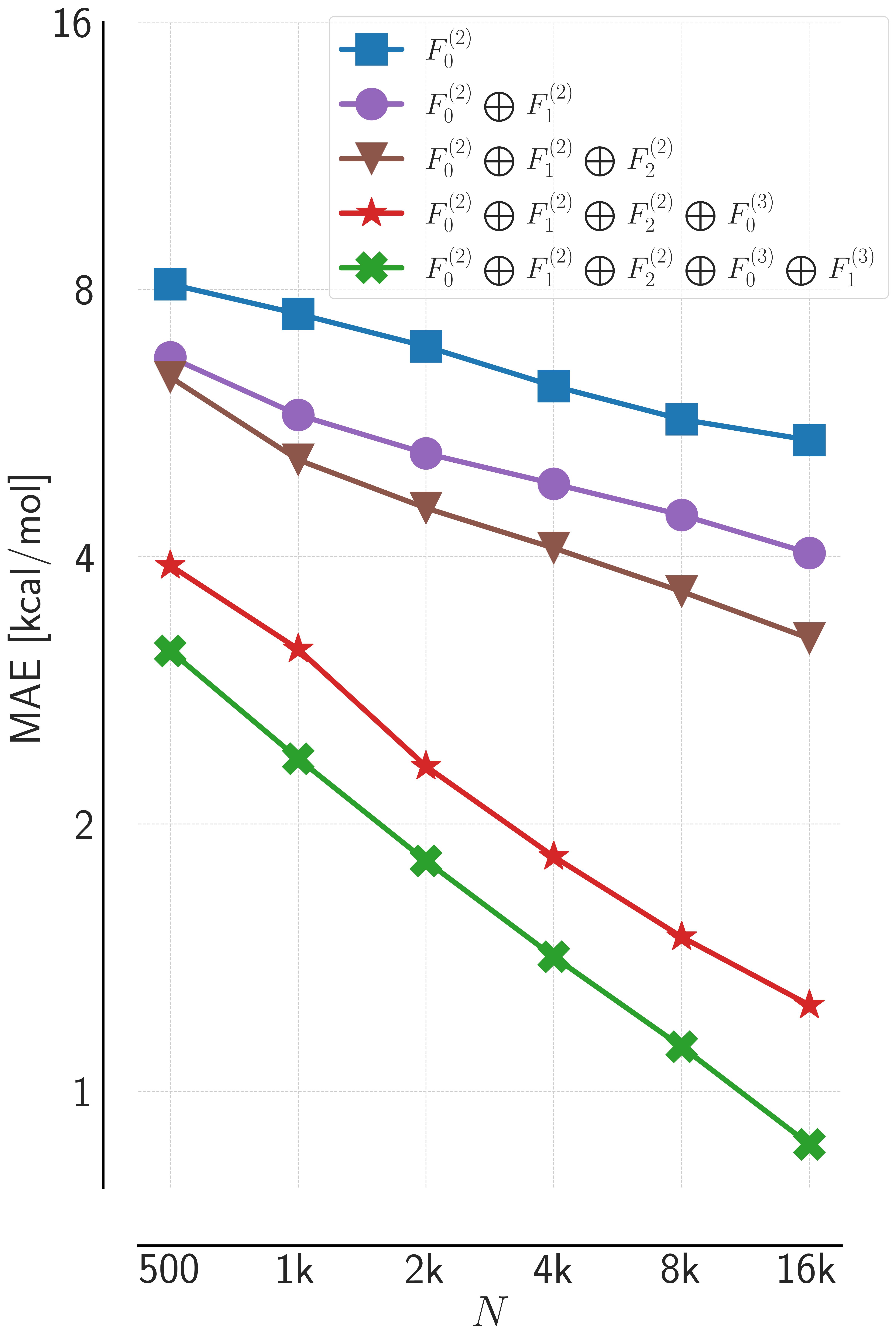
It is apparent that both the derivative and many-body terms improve the learning capacity, albeit by different magnitudes.

Throughout our testing on the QM7⁴⁹, QM9⁴⁸ and QMugs⁵⁰ datasets, we have found these 2, 3-body functionals to be sufficient at discriminating between all of the molecular structures. Cases where the 2-body information does not suffice include homometric pairs, as already discussed many years ago ¹⁴. And even 3- and 4-body information does not suffice for some cases, as recently discussed in Ref. 51. We note here that, whenever necessary, arbitrarily higher order derivative and many-body information could also be included in MBDFs at minimal increase in size, i.e. one additional term per order (See eq. (8)). In particular, we believe that the inclusion of the 4-body term as a functional of the dihedrals could further improve the learning capacity for conformational isomers. Inclusion of 4-body information has been shown to result in further improvements of learning curves ⁵². Also note that the size of MBDF is invariant to the cutoffs used which can be raised to arbitrarily higher values while employing a suitable long-range functional (hence increasing the farsightedness of the representation) without affecting the kernel evaluation cost. We further note that other weighting functions and response terms could also be useful for QML models of physical observables such as dipole moments, vibrational frequencies, heat capacities etc.

MBDF is a local representation and its size scales linearly with the number of atoms in the system. In order to eliminate this scaling we can transform to the frequency space of MBDF functional values. The frequencies can be evaluated by normalizing the functional values to lie within an arbitrary range and then using, for e.g., kernel density estimation⁵³. For a finite set of MBDF functional values $\{X_{i}\}_{i=1}^{5M}$ over the range $[a,b]$, a ”smooth histogram” of their frequencies can be constructed by placing a set of kernel functions $K$ at each point $X_{i}$:

$\displaystyle f(u)=\frac{1}{5M}~\sum_{i=1}^{5M}~K(u,X_{i})$

(17)

where $f(u)$ gives the density of the samples at any point $u~\epsilon~[a,b]$. If the set $\{X_{i}\}_{i=1}^{5M}$ are the MBDF functional values for any molecule, their distribution density can be evaluated using eq. (17). The density $f(u)$ can then be used as a global molecular representation whose size is independent of the number of MBDF functional values, and number of atoms by extension. The (dis-)similarity between two molecules $A$ and $B$ can be evaluated as, e.g., the l2-distance:

$\displaystyle d(A,B)^{2}=\int_{-c}^{c}du~|f_{A}(u)-f_{B}(u)|^{2}$

(18)

where $[-c,c]$ is the normaliztion range chosen as $[-10,10]$ in our work. The form of the density function used in our work is:

$\displaystyle f_{A}(u)=\frac{1}{5M}~\sum_{i=1}^{5M}~\frac{\sqrt{|X_{i}|}}{\sqrt{2\pi}\sigma_{b}}~\exp{\left(-\frac{(u-X_{i})^{2}}{2\sigma_{b}^{2}}\right)}$

(19)

where $X_{i}$ are MBDF functionals for molecule $A$, $\sigma_{b}$ is the variance of the Gaussian function and is a hyperparameter (also called bandwidth). Comparing with eq. (17), the function $K$ is defined as:

$\displaystyle K(u,X_{i}):=\frac{\sqrt{|X_{i}|}}{\sqrt{2\pi}\sigma_{b}}~\exp{\left(-\frac{(u-X_{i})^{2}}{2\sigma_{b}^{2}}\right)}$

(20)

Note that this is a divergence⁵⁴ but not a kernel function because it is asymmetric:

	$\displaystyle K(x,y)=$	$\displaystyle\frac{\sqrt{|y|}}{\sqrt{2\pi}\sigma_{b}}~\exp{\left(-\frac{(x-y)^{2}}{2\sigma_{b}^{2}}\right)}$
	$\displaystyle\begin{split}\neq&\frac{\sqrt{|x|}}{\sqrt{2\pi}\sigma_{b}}~\exp{\left(-\frac{(x-y)^{2}}{2\sigma_{b}^{2}}\right)}=K(y,x)\end{split}$			(21)

This function is used because it weights the MBDF functional frequencies by the functional value itself resulting in the distance measurement (eq. (18)) being weighted by the difference in functional values. Another advantage of this function is that it eliminates the frequency of null values (or ”ghost atoms”) within the MBDF representation which might be present due to the procedure of zero-padding¹.
In our work we generate a separate density function $f(u)$ for each of the 5 MBDF functionals in eq. (11-15), and for each unique chemical element present in the dataset. These are then concatenated to form the global representation of the molecule. Alternatively, it could be done by using multivariate Gaussian functions for the density estimation. Let $\mathbf{x}_{i}$ denote the 5-dimensional vector of MBDF functional values (eq. 11-15) for any atom $i$ in molecule $A$. Then the multivariate density function $f_{A}(\mathbf{u})$ of this molecule can be evaluated as :

$\displaystyle f_{A}(\mathbf{u})=\frac{1}{M}~\sum_{i=1}^{M}~K(\mathbf{u},\mathbf{x}_{i})$

(22)

$\displaystyle f_{A}(\mathbf{u})=\frac{1}{M}\sum_{i=1}^{M}\frac{(\mathbf{x}_{i}^{T}\mathbf{x}_{i})^{1/4}}{\sqrt{2\pi}\sigma_{b}}\exp{\left(-\frac{(\mathbf{u}-\mathbf{x}_{i})^{T}(\mathbf{u}-\mathbf{x}_{i})}{2\sigma_{b}^{2}}\right)}$

(23)

The l2-distance between molecules $A$ and $B$ then takes the form:

$$d(A,B)^{2}=\int d\mathbf{u}~(f_{A}(\mathbf{u})-f_{B}(\mathbf{u}))^{T}(f_{A}(\mathbf{u})-f_{B}(\mathbf{u}))$$

(24)

where the integral is over the normalization region. Since the former method generates a more compact representation we have chosen to work with it. The abbreviation DF (Density of functionals) will be used throughout for this global representation.

The DF method allows generating a representation that does not scale with the number of atoms in the system. However, in order to use it as a feature vector the density functions have to be discretized. Through convergence testing we have set the grid spacing to 0.2 throughout our work. However, we note that this grid spacing could be changed for a different data-set in order to achieve the desirable accuracy vs computational cost trade-off. Furthermore, DF corresponds to a flattened feature vector which can be used with global kernels (or other ML methods), and which exhibits superior performance when compared to a straightforward concatenation of all MBDF rows (see Figure 2). The flattened MBDF representation is generated by sorting the MBDF matrix of each molecule by the row norm, and then flattening the matrix by concatenation of the rows to vectorize it¹.

Figure 3 shows molecular fingerprints generated using the 1 and 5 functional DF representations for three diverse and relevant organic molecules (glucose, uric acid, and testosterone) on the same grid. For each molecule, a distinct fingerprint is obtained, with peak-positions depending on the local chemical environment of each atom. Consequently, peaks of atoms with chemically similar environments are located closer to each other. Peak heights encode both number and type (because of the density estimate being weighted) of chemical environments [See Eq. 20]. Figure 3 demonstrates that for molecules with increasing size, corresponding DF based fingerprints will grow in magnitude, not in size. In the SI, we also show how DF fingerprints distinguish conformational isomers, as exemplified for the chair and boat conformations of cyclohexane.

The ML method that we focus on, and use throughout this work, is the supervised learning method called Kernel ridge regression^{18; 39} (KRR). This method has been covered extensively earlier^{1; 35; 34; 3; 2} so we skip the details here.

The kernel functions^{55; 56} we use in our work along with global representations are the Gaussian kernel,

$\displaystyle k(\mathbf{x}_{I},\mathbf{x}_{J})=\exp{\left(-\frac{||\mathbf{x}_{I}-\mathbf{x}_{J}||^{2}_{2}}{2\sigma^{2}}\right)}$

(25)

and Laplacian kernel,

$\displaystyle k(\mathbf{x}_{I},\mathbf{x}_{J})=\exp{\left(-\frac{||\mathbf{x}_{I}-\mathbf{x}_{J}||_{1}}{\sigma}\right)}$

(26)

where $\mathbf{x}_{I}$ denotes the representation vector of molecule $I$.
The kernel function used for the local representations FCHL19, SOAP and MBDF is a summation of atomic kernels:

$\displaystyle k(\mathbf{M}_{I},\mathbf{M}_{J})=\sum_{a\epsilon i}\sum_{b\epsilon j}k^{l}(\mathbf{x}_{Ia},\mathbf{x}_{Jb})$

(27)

with the local Gaussian kernel:

$\displaystyle k^{l}(\mathbf{x}_{Ia},\mathbf{x}_{Jb})=\mathbf{\delta}_{Z_{a},Z_{b}}\exp{\left(-\frac{||\mathbf{x}_{Ia}-\mathbf{x}_{Jb}||^{2}_{2}}{2\sigma^{2}}\right)}~$

(28)

the local Laplacian kernel:

$\displaystyle k^{l}(\mathbf{x}_{Ia},\mathbf{x}_{Jb})=\mathbf{\delta}_{Z_{a},Z_{b}}\exp{\left(-\frac{||\mathbf{x}_{Ia}-\mathbf{x}_{Jb}||_{1}}{\sigma}\right)}~$

(29)

or the local exponential kernel with the Euclidean norm:

$\displaystyle k^{l}(\mathbf{x}_{Ia},\mathbf{x}_{Jb})=\mathbf{\delta}_{Z_{a},Z_{b}}\exp{\left(-\frac{||\mathbf{x}_{Ia}-\mathbf{x}_{Jb}||_{2}}{\sigma}\right)}~$

(30)

where $\mathbf{M}_{I}$ denotes the representation matrix of molecule $I$, $\mathbf{x}_{Ia}$ denotes the representation vector of atom $a$ within molecule $I$ and $\mathbf{\delta}_{Z_{a},Z_{b}}$ denotes a Kronecker Delta over the nuclear charges $Z_{a},Z_{b}$ which restricts the similarity measurement between atoms of the same chemical element³⁴. Other kernel functions will also be tested in the future^{57; 58; 40}.
Throughout this study, we evaluate performance of ML methods through learning curves for the task of predicting physical properties of molecular systems. Learning curves quantify the model prediction error $\varepsilon$ (often measured as mean absolute error (MAE)) against the number of training samples $N$ and are key to understand the efficiency of ML models. It is generally known^{18; 59; 60} that they are linear on a log-log scale,

$\displaystyle\log{\left(\varepsilon\right)}\approx I+S\log{(N)}~$

(31)

where $I$ is the initial error and $S$ is the slope indicating model improvement given more training data. We also note that according to the central limit theorem the distribution of the errors $\epsilon$ approaches the normal distribution with standard deviation $\frac{\sigma}{\sqrt{N}}$, and mean 0 as $N\xrightarrow{}\infty$. Hence eq. (31) becomes :

$\displaystyle\log{\left(\varepsilon\right)}\approx\log(\sigma)-\frac{1}{2}\log{(N)}$

(32)

The current form of the representations has been optimized for Kernel based learning models. It depends on the weighting functions used and a number of hyperparameters which include variances ($\sigma_{r},\sigma_{\theta}$) of the Gaussian PDFs, weighting function hyperparameters mentioned in eq. (12)-(16), and bandwidth $\sigma_{b}$ for the DF representation. The hyperparameter optimization was done on a random subset of two thousand molecules from the QM7 dataset⁴⁹, and then kept fixed for all other data-sets. We note that further improvements might be possible if they had been optimized simultaneously on all data-sets. The weighting functions $g_{n}(\tau)$ in eq. (8) were chosen by straightforward screening of the functions mentioned earlier. The optimization minimized the atomization energy prediction errors on the QM7 subset using Gaussian Process (GP) based Bayesian Optimization (BOpt)³⁹. Starting with a Gaussian prior, the method fits a posterior distribution over the objective function using successive function evaluations. The posterior distribution is then used to construct an efficient acquisition function which can be optimized using, for instance, a quasi-Newton method to determine the next query point. Table 1 shows the optimized hyperparameter values used throughout this work.

We used the scikit-optimize⁶¹ implementation of GP based BOpt using the default Matérn kernel with unit variance and the limited memory BFGS optimizer⁶² for the acquisition function. In order to enable comparison to other representations (such as FCHL or SOAP) that rely on distance cutoffs, we have chosen to set inter-atomic distance cutoff $r_{c}$ for MBDF to 6 Å throughout this work. We note that larger cutoffs for MBDF would not change its size.

All MBDF functionals were evaluated using the trapezoidal numerical integration method. The grid spacing for discretizing DF densities has been set to 0.2 throughout our work as noted earlier. The bandwidth $\sigma_{b}$ = 0.07 was found to work well on the QM7 subset however it is recommended to be screened once (in the range $\sim$ [0.01,1]) along with the grid-spacing when using with other datasets. The Numpy⁶³ and Numba⁶⁴ libraries are used in the representation generation code.

The QM9 dataset⁴⁸ consists of $\sim$134k small organic molecules with up to 9 heavy atoms (C, N, O, F). The calculations were performed at the B3LYP/6-31G(2df,p)^{65; 66; 67} level of theory.
QMugs is a dataset containing $\sim$665k biologically and pharmacologically relevant drug-like molecules. It consists of larger molecules than QM9 with up to 100 heavy atoms (C, N, O, F, P, S, Cl, Br, or I) per molecule. The training and predictions were performed on the DFT ($\omega$B97X-D/def2-SVP)^{68; 69} values reported in the dataset. The QMugs subsets we used for Figure 5 were drawn at random and consist of 20k molecules. Throughout, we used zero-padding for all representations studied in order to accommodate training and test molecules smaller than the maximum present in the data.

In order to keep the FCHL19 and SOAP kernel evaluations computationally tractable, we have (a) restricted ourselves to a maximum 100 atoms per QMugs-molecule, and (b) reduced the default hyperparameters of the FCHL19 and SOAP representations to nRs2 = 12, nRs3 = 10, $r_{cut}$ = 6$\mathrm{\AA}$ and $n_{max}$ = $l_{max}$ = 3, $\sigma$ = 0.1, $r_{cut}$ = 6$\mathrm{\AA}$, respectively. For consistency, we used the same parameters for all other results reported in this article. These two versions of the representations with the reduced basis sets are denoted as FCHL19* and SOAP* in all reported figures. Note that the latter choice of hyperparameters negligibly deteriorates the predictive accuracy for QM9 (as assessed below and when comparing to the published prediction errors on QM9 for FCHL19 and SOAP2013). For FCHL19 and SOAP based prediction errors reported here within for QMugs, it could still be that the accuracy could improve further if these parameters were optimized.

Figure 4 also includes results for QML models based on the 2- (k = 2) and 3-body (k = 3) Many-Body Tensor Representations (MBTR)²² and a variant⁷⁰ of the Atom Centered Symmetry Functions²⁰ (ACSF) as implemented in the QMLcode library⁷¹. The MBTR representations were generated with the same hyperparameters as those used in Ref.33 for the 10k training point on the QM9 dataset.

Throughout our work, the FCHL19, SLATM and ACSF representations were generated using the QMLcode library⁷¹, SOAP was generated using the Dscribe library⁷² with the default gaussian type radial basis functions, MBTR was generated using the qmmlpack library⁷³ and SchNet⁷⁴, PaiNN⁷⁵ were built and trained using the SchNetPack⁷⁶ libray. Allegro⁷⁷ was built and trained using the nequip⁷⁸ code⁷⁹ based on the E(3)-NN framework^{80; 81}.
For FCHL19, SOAP and ACSF we employed the local Gaussian (eq. (28)), for SLATM, MBTR and DF we use the global Gaussian (eq. (25)) and for CM, BOB we use the global Laplacian (eq. (26)) kernels respectively. For MBDF we used the local Gaussian kernel on the MD17 dataset and the local exponential (eq. (30)) kernel for all other models. These choices were made based on the best performances for each representation. All kernel evaluations were performed using the QMLcode library.

Figure 6 shows scaling plots of kernel evaluation timings across both QM9 and QMugs datasets for various representations and as a function of training set size. As one would expect, the off-set increases systematically with increasing representation and training molecule size. More specifically, for the larger molecules of QMugs, the FCHL19 and SOAP kernel evaluations become rapidly intractable very quickly with the 16k kernel (Fig. 5) already taking an entire compute node day. Encouragingly and in stark contrast, DF, being a size invariant representation, shows hardly any change in computational overhead when moving from the small QM9 molecules to the much larger QMugs molecules.

For context, the time required in the kernel inversion step for each training kernel is shown as well. The bottleneck crossover from kernel generation ($\mathcal{O}(n^{2})$) to the inversion step ($\mathcal{O}(n^{3})$) occurs rather late. When using Cholesky decomposition it occurs for MBDF at $N\sim$ 64k training molecules. For less compact representations (for SLATM and larger) the same cross-over occurs at training set sizes that exceed $\sim$1 M. As demonstrated above, chemical accuracy is already achieved at substantially smaller training set sizes. Consequently and contrary to popular belief, for any of the more modern and accurate representations, kernel inversion does not constitute a bottleneck.

Table 2 reports the kernel evaluation and representation generation timings for both the QM9 dataset (130k molecules) and the QMugs subset (20k molecules) used in our work. It can be seen that MBDF reduces the local kernel evaluation timings from days to a few minutes for both small and large molecules. For the representation generation step we note that our code is currently written in Python and uses the Numba⁶⁴ library and could be further optimized with a low-level implementation. However, the current timings as well do not affect the overall QML model cost much given the kernel evaluation bottleneck.

We assessed the generalization capacities of MBDF/DF on physical properties other than atomization energies. Figure 7 shows the learning curves for the task of predicting 8 important molecular quantum properties from the QM9 dataset. These include the highest occupied molecular orbital (HOMO), lowest unoccupied molecular orbital (LUMO) eigenvalues and the HOMO-LUMO gap, internal energy at 0 K ($U_{0}$), dipole moment norm ($|\boldsymbol{\mu}|$), static isotropic polarizability ($\alpha$), zero point vibrational energy (ZPVE) and heat capacity ($C_{v}$). Due to substantial computational costs, the KRR hyper-parameters were not optimized at each training size for the FCHL19 and SOAP representations, and we picked the same parameters as those used for learning atomization energies in figure 4. We reproduce earlier trends among intensive and extensive properties when using local/global kernels ^{93; 3}. MBDF and DF match this trend: They perform better on extensive and on intensive properties, respectively.

Again, note that the performance on these properties of MBDF/DF could be further improved by including different functionals suited to the property, or by augmenting them with response terms as was done for the FCHL19 representation⁹³. It would also be interesting to see how the learning capacities across these different physical properties is affected by the inclusion of higher order functional terms.

References

- Rupp et al. (2012a) M. Rupp, A. Tkatchenko, K.-R. Müller, and O. A. von Lilienfeld, Phys. Rev. Lett. 108, 058301 (2012a).
- von Lilienfeld (2018) O. A. von Lilienfeld, Angewandte Chemie International Edition 57, 4164 (2018), http://dx.doi.org/10.1002/anie.201709686.
- Faber et al. (2017) F. A. Faber, L. Hutchison, B. Huang, J. Gilmer, S. S. Schoenholz, G. E. Dahl, O. Vinyals, S. Kearnes, P. F. Riley, and O. A. von Lilienfeld, Journal of Chemical Theory and Computation 13, 5255 (2017), pMID: 28926232, https://doi.org/10.1021/acs.jctc.7b00577 .
- Ho and Rabitz (1996) T. Ho and H. Rabitz, J. Chem. Phys. 104, 2584 (1996).
- Manzhos and Carrington, Jr. (2006) S. Manzhos and T. Carrington, Jr., J. Chem. Phys. 125, 084109 (2006).
- Behler and Parrinello (2007) J. Behler and M. Parrinello, Phys. Rev. Lett. 98, 146401 (2007).
- Bartók et al. (2010) A. P. Bartók, M. C. Payne, R. Kondor, and G. Csányi, Phys. Rev. Lett. 104, 136403 (2010).
- Handley and Popelier (2010) C. M. Handley and P. L. A. Popelier, The Journal of Physical Chemistry A 114, 3371 (2010), pMID: 20131763, https://doi.org/10.1021/jp9105585 .
- Smith et al. (2017) J. S. Smith, O. Isayev, and A. E. Roitberg, Chem. Sci. 8, 3192 (2017).
- Snyder et al. (2012) J. C. Snyder, M. Rupp, K. Hansen, K.-R. Müller, and K. Burke, Phys. Rev. Lett. 108, 253002 (2012).
- Pozun et al. (2012) Z. D. Pozun, K. Hansen, D. Sheppard, M. Rupp, K.-R. Müller, and G. Henkelman, J. Chem. Phys. 136, 174101 (2012).
- Ceriotti et al. (2021a) M. Ceriotti, C. Clementi, and O. Anatole von Lilienfeld, Chem. Rev. 121, 9719 (2021a).
- Ceriotti et al. (2021b) M. Ceriotti, C. Clementi, and O. Anatole von Lilienfeld, The Journal of Chemical Physics 154, 160401 (2021b), https://doi.org/10.1063/5.0051418 .
- von Lilienfeld et al. (2015) O. A. von Lilienfeld, R. Ramakrishnan, M. Rupp, and A. Knoll, International Journal of Quantum Chemistry 115, 1084 (2015), https://onlinelibrary.wiley.com/doi/pdf/10.1002/qua.24912 .
- Ghiringhelli et al. (2015) L. M. Ghiringhelli, J. Vybiral, S. V. Levchenko, C. Draxl, and M. Scheffler, Phys. Rev. Lett. 114, 105503 (2015).
- Musil et al. (2021) F. Musil, A. Grisafi, A. P. Bartók, C. Ortner, G. Csányi, and M. Ceriotti, Chemical Reviews 121, 9759 (2021), pMID: 34310133, https://doi.org/10.1021/acs.chemrev.1c00021 .
- Ramakrishnan and von Lilienfeld (2015) R. Ramakrishnan and O. A. von Lilienfeld, CHIMIA 69, 182 (2015).
- Vapnik (1998) V. N. Vapnik, Statistical Learning Theory (Wiley-Interscience, 1998).
- Collins et al. (2018) C. R. Collins, G. J. Gordon, O. A. von Lilienfeld, and D. J. Yaron, The Journal of Chemical Physics 148, 241718 (2018), https://doi.org/10.1063/1.5020441 .
- Behler (2011) J. Behler, The Journal of Chemical Physics 134, 074106 (2011), https://doi.org/10.1063/1.3553717 .
- Zhu et al. (2016) L. Zhu, M. Amsler, T. Fuhrer, B. Schaefer, S. Faraji, S. Rostami, S. A. Ghasemi, A. Sadeghi, M. Grauzinyte, C. Wolverton, and S. Goedecker, The Journal of Chemical Physics 144, 034203 (2016), https://doi.org/10.1063/1.4940026 .
- Huo and Rupp (2022) H. Huo and M. Rupp, Machine Learning: Science and Technology 3, 045017 (2022).
- Gastegger et al. (2018) M. Gastegger, L. Schwiedrzik, M. Bittermann, F. Berzsenyi, and P. Marquetand, The Journal of Chemical Physics 148, 241709 (2018), https://doi.org/10.1063/1.5019667 .
- Drautz (2019) R. Drautz, Phys. Rev. B 99, 014104 (2019).
- Braams and Bowman (2009) B. J. Braams and J. M. Bowman, International Reviews in Physical Chemistry 28, 577 (2009), https://doi.org/10.1080/01442350903234923 .
- Hirn et al. (2015) M. J. Hirn, N. Poilvert, and S. Mallat, CoRR abs/1502.02077 (2015), 1502.02077 .
- Shapeev (2016) A. V. Shapeev, Multiscale Modeling & Simulation 14, 1153 (2016), https://doi.org/10.1137/15M1054183 .
- Nigam et al. (2020) J. Nigam, S. Pozdnyakov, and M. Ceriotti, The Journal of Chemical Physics 153, 121101 (2020), https://doi.org/10.1063/5.0021116 .
- Zaverkin and Kästner (2020) V. Zaverkin and J. Kästner, Journal of Chemical Theory and Computation 16, 5410 (2020), pMID: 32672968, https://doi.org/10.1021/acs.jctc.0c00347 .
- Jinnouchi et al. (2020) R. Jinnouchi, F. Karsai, C. Verdi, R. Asahi, and G. Kresse, The Journal of Chemical Physics 152, 234102 (2020), https://doi.org/10.1063/5.0009491 .
- Thompson et al. (2015) A. Thompson, L. Swiler, C. Trott, S. Foiles, and G. Tucker, Journal of Computational Physics 285, 316 (2015).
- Willatt et al. (2018) M. J. Willatt, F. Musil, and M. Ceriotti, Phys. Chem. Chem. Phys. 20, 29661 (2018).
- Langer et al. (2022) M. F. Langer, A. Goeßmann, and M. Rupp, npj Computational Materials 8, 41 (2022).
- Christensen et al. (2020) A. S. Christensen, L. A. Bratholm, F. A. Faber, and O. Anatole von Lilienfeld, The Journal of Chemical Physics 152, 044107 (2020), https://doi.org/10.1063/1.5126701 .
- Faber et al. (2018) F. A. Faber, A. S. Christensen, B. Huang, and O. A. von Lilienfeld, The Journal of Chemical Physics 148, 241717 (2018), https://doi.org/10.1063/1.5020710 .
- Bartók et al. (2013) A. P. Bartók, R. Kondor, and G. Csányi, Phys. Rev. B 87, 184115 (2013).
- Huang and von Lilienfeld (2017) B. Huang and O. A. von Lilienfeld, “Quantum machine learning using atom-in-molecule-based fragments selected on-the-fly,” (2017).
- Hansen et al. (2015) K. Hansen, F. Biegler, R. Ramakrishnan, W. Pronobis, O. A. von Lilienfeld, K.-R. Müller, and A. Tkatchenko, The Journal of Physical Chemistry Letters 6, 2326 (2015), pMID: 26113956, https://doi.org/10.1021/acs.jpclett.5b00831 .
- Rasmussen and Williams (2006) C. E. Rasmussen and C. K. I. Williams, Gaussian processes for machine learning., Adaptive computation and machine learning (MIT Press, 2006) pp. I–XVIII, 1–248.
- De et al. (2016) S. De, A. P. Bartók, G. Csányi, and M. Ceriotti, Phys. Chem. Chem. Phys. 18, 13754 (2016).
- Bartók and Csányi (2015) A. P. Bartók and G. Csányi, International Journal of Quantum Chemistry 115, 1051 (2015).
- Chmiela et al. (2023) S. Chmiela, V. Vassilev-Galindo, O. T. Unke, A. Kabylda, H. E. Sauceda, A. Tkatchenko, and K.-R. Müller, Science Advances 9, eadf0873 (2023), https://www.science.org/doi/pdf/10.1126/sciadv.adf0873 .
- Faber et al. (2016) F. A. Faber, A. Lindmaa, O. A. von Lilienfeld, and R. Armiento, Phys. Rev. Lett. 117, 135502 (2016).
- Morse (1929) P. M. Morse, Phys. Rev. 34, 57 (1929).
- Jones (1924) J. E. Jones, Proceedings of the Royal Society of London. Series A (1924).
- Axilrod and Teller (1943) B. M. Axilrod and E. Teller, The Journal of Chemical Physics 11, 299 (1943), https://doi.org/10.1063/1.1723844 .
- Stillinger and Weber (1985) F. H. Stillinger and T. A. Weber, Phys. Rev. B 31, 5262 (1985).
- Ramakrishnan et al. (2014) R. Ramakrishnan, P. O. Dral, M. Rupp, and O. A. von Lilienfeld, Scientific Data 1 (2014).
- Rupp et al. (2012b) M. Rupp, A. Tkatchenko, K.-R. Müller, and O. A. von Lilienfeld, Phys. Rev. Lett. 108, 058301 (2012b).
- Isert et al. (2022) C. Isert, K. Atz, J. Jiménez-Luna, and G. Schneider, Scientific Data 9, 273 (2022).
- Pozdnyakov et al. (2020) S. N. Pozdnyakov, M. J. Willatt, A. P. Bartók, C. Ortner, G. Csányi, and M. Ceriotti, Phys. Rev. Lett. 125, 166001 (2020).
- Huang and von Lilienfeld (2016) B. Huang and O. A. von Lilienfeld, The Journal of Chemical Physics 145, 161102 (2016), https://doi.org/10.1063/1.4964627 .
- Parzen (1962) E. Parzen, The Annals of Mathematical Statistics 33, 1065 (1962).
- Amari and Nagaoka (2000) S.-i. Amari and H. Nagaoka, Methods of information geometry, Vol. 191 (American Mathematical Soc., 2000).
- Deisenroth et al. (2020) M. P. Deisenroth, A. A. Faisal, and C. S. Ong, Mathematics for Machine Learning (Cambridge University Press, 2020).
- Schütt et al. (2020) K. T. Schütt, S. Chmiela, O. A. von Lilienfeld, A. Tkatchenko, K. Tsuda, and K.-R. Müller, Machine Learning Meets Quantum Physics (Springer, 2020).
- Çaylak et al. (2020) O. Çaylak, O. A. von Lilienfeld, and B. Baumeier, Machine Learning: Science and Technology 1, 03LT01 (2020).
- Fabregat et al. (2022) R. Fabregat, P. van Gerwen, M. Haeberle, F. Eisenbrand, and C. Corminboeuf, Machine Learning: Science and Technology 3, 035015 (2022).
- Cortes et al. (1994) C. Cortes, L. D. Jackel, S. A. Solla, V. Vapnik, and J. S. Denker, in Advances in Neural Information Processing Systems (1994) pp. 327–334.
- Müller et al. (1996) K. R. Müller, M. Finke, N. Murata, K. Schulten, and S. Amari, Neural Comp. 8, 1085 (1996).
- Head et al. (2021) T. Head, M. Kumar, H. Nahrstaedt, G. Louppe, and I. Shcherbatyi, “scikit-optimize/scikit-optimize,” (2021).
- Liu and Nocedal (1989) D. C. Liu and J. Nocedal, Mathematical Programming 45, 503 (1989).
- Harris et al. (2020) C. R. Harris, K. J. Millman, S. J. van der Walt, R. Gommers, P. Virtanen, D. Cournapeau, E. Wieser, J. Taylor, S. Berg, N. J. Smith, R. Kern, M. Picus, S. Hoyer, M. H. van Kerkwijk, M. Brett, A. Haldane, J. F. del Río, M. Wiebe, P. Peterson, P. Gérard-Marchant, K. Sheppard, T. Reddy, W. Weckesser, H. Abbasi, C. Gohlke, and T. E. Oliphant, Nature 585, 357 (2020).
- Lam et al. (2015) S. K. Lam, A. Pitrou, and S. Seibert, in Proceedings of the Second Workshop on the LLVM Compiler Infrastructure in HPC, LLVM ’15 (Association for Computing Machinery, New York, NY, USA, 2015).
- Becke (1993) A. D. Becke, The Journal of Chemical Physics 98, 5648 (1993), https://doi.org/10.1063/1.464913 .
- Lee et al. (1988) C. Lee, W. Yang, and R. G. Parr, Phys. Rev. B 37, 785 (1988).
- Petersson et al. (1988) G. A. Petersson, A. Bennett, T. G. Tensfeldt, M. A. Al‐Laham, W. A. Shirley, and J. Mantzaris, The Journal of Chemical Physics 89, 2193 (1988), https://doi.org/10.1063/1.455064 .
- Chai and Head-Gordon (2008) J.-D. Chai and M. Head-Gordon, Phys. Chem. Chem. Phys. 10, 6615 (2008).
- Weigend and Ahlrichs (2005) F. Weigend and R. Ahlrichs, Phys. Chem. Chem. Phys. 7, 3297 (2005).
- Yao et al. (2018) K. Yao, J. E. Herr, D. W. Toth, R. Mckintyre, and J. Parkhill, Chemical Science 9, 2261 (2018).
- Christensen et al. (2017) A. S. Christensen, L. A. Bratholm, F. A. Faber, B. Huang, A. Tkatchenko, K. R. Müller, and O. A. von Lilienfeld, “Qml: A python toolkit for quantum machine learning,” (2017).
- Himanen et al. (2020) L. Himanen, M. O. J. Jäger, E. V. Morooka, F. Federici Canova, Y. S. Ranawat, D. Z. Gao, P. Rinke, and A. S. Foster, Computer Physics Communications 247, 106949 (2020).
- Rupp (2015) M. Rupp, International Journal of Quantum Chemistry 115, 1058 (2015).
- Schütt et al. (2018) K. T. Schütt, P. Kessel, M. Gastegger, K. A. Nicoli, A. Tkatchenko, and K.-R. Müller, Journal of Chemical Theory and Computation 15, 448 (2018).
- Schütt et al. (2021) K. T. Schütt, O. T. Unke, and M. Gastegger, CoRR abs/2102.03150 (2021), 2102.03150 .
- Schütt et al. (2017) K. Schütt, P.-J. Kindermans, H. E. Sauceda Felix, S. Chmiela, A. Tkatchenko, and K.-R. Müller, in Advances in Neural Information Processing Systems, Vol. 30, edited by I. Guyon, U. V. Luxburg, S. Bengio, H. Wallach, R. Fergus, S. Vishwanathan, and R. Garnett (Curran Associates, Inc., 2017).
- Musaelian et al. (2023) A. Musaelian, S. Batzner, A. Johansson, L. Sun, C. J. Owen, M. Kornbluth, and B. Kozinsky, Nature Communications 14 (2023), 10.1038/s41467-023-36329-y.
- Batzner et al. (2022) S. Batzner, A. Musaelian, L. Sun, M. Geiger, J. P. Mailoa, M. Kornbluth, N. Molinari, T. E. Smidt, and B. Kozinsky, Nature Communications 13 (2022), 10.1038/s41467-022-29939-5.
- Geiger et al. (2022a) M. Geiger, T. Smidt, M. Alby, B. K. Miller, W. Boomsma, B. Dice, K. Lapchevskyi, M. Weiler, Michał Tyszkiewicz, M. Uhrin, S. Batzner, D. Madisetti, J. Frellsen, N. Jung, S. Sanborn, Jkh, Mingjian Wen, J. Rackers, M. Rød, and M. Bailey, “e3nn/e3nn: 2022-12-12,” (2022a).
- Geiger et al. (2022b) M. Geiger, T. Smidt, A. M., B. K. Miller, W. Boomsma, B. Dice, K. Lapchevskyi, M. Weiler, M. Tyszkiewicz, S. Batzner, D. Madisetti, M. Uhrin, J. Frellsen, N. Jung, S. Sanborn, M. Wen, J. Rackers, M. Rød, and M. Bailey, “Euclidean neural networks: e3nn,” (2022b).
- Geiger and Smidt (2022) M. Geiger and T. Smidt, “e3nn: Euclidean neural networks,” (2022).
- Townsend et al. (2020) J. Townsend, C. P. Micucci, J. H. Hymel, V. Maroulas, and K. D. Vogiatzis, Nature Communications 11, 3230 (2020).
- Bigi et al. (2023) F. Bigi, S. N. Pozdnyakov, and M. Ceriotti, “Wigner kernels: body-ordered equivariant machine learning without a basis,” (2023), arXiv:2303.04124 [physics.chem-ph] .
- Browning et al. (2022) N. J. Browning, F. A. Faber, and O. Anatole von Lilienfeld, The Journal of Chemical Physics 157, 214801 (2022).
- Atz et al. (2022) K. Atz, C. Isert, M. N. Böcker, J. Jiménez-Luna, and G. Schneider, Physical Chemistry Chemical Physics 24, 10775 (2022).
- Bannwarth et al. (2019) C. Bannwarth, S. Ehlert, and S. Grimme, Journal of Chemical Theory and Computation 15, 1652 (2019).
- Montavon et al. (2013) G. Montavon, M. Rupp, V. Gobre, A. Vazquez-Mayagoitia, K. Hansen, A. Tkatchenko, K.-R. Müller, and O. A. von Lilienfeld, New Journal of Physics 15, 095003 (2013).
- Blum and Reymond (2009) L. C. Blum and J.-L. Reymond, J. Am. Chem. Soc. 131, 8732 (2009).
- Christensen and von Lilienfeld (2020) A. S. Christensen and O. A. von Lilienfeld, Machine Learning: Science and Technology 1, 045018 (2020).
- Christensen and lilienfeld (2020) A. S. Christensen and A. V. lilienfeld, (2020), 10.6084/m9.figshare.12672038.v3.
- Chmiela et al. (2017) S. Chmiela, A. Tkatchenko, H. E. Sauceda, I. Poltavsky, K. T. Schütt, and K.-R. Müller, Science Advances 3 (2017), 10.1126/sciadv.1603015.
- Chmiela et al. (2018) S. Chmiela, H. E. Sauceda, K.-R. Müller, and A. Tkatchenko, Nature Communications 9 (2018), 10.1038/s41467-018-06169-2.
- Christensen et al. (2019) A. S. Christensen, F. A. Faber, and O. A. von Lilienfeld, The Journal of Chemical Physics 150, 064105 (2019), https://doi.org/10.1063/1.5053562 .