Modeling and forecasting age-specific drug overdose mortality in the United States

Lucas Böttcher Email: l.boettcher@fs.de Affiliation: Dept. of Computational Science and Philosophy, Frankfurt School of Finance and Management, Frankfurt am Main, 60322, Germany Tom Chou Affiliation: Dept. of Computational Medicine, UCLA, Los Angeles, CA 90095-1766 Affiliation: Dept. of Mathematics, UCLA, Los Angeles, CA 90095-1555 Maria R. D’Orsogna Affiliation: Dept. of Mathematics, California State University at Northridge, Los Angeles, CA 91330-8313 Affiliation: Dept. of Computational Medicine, UCLA, Los Angeles, CA 90095-1766

August 11, 2026

Abstract

Drug overdose deaths continue to increase in the United States for all major drug categories. Over the past two decades the total number of overdose fatalities has increased more than five-fold; since 2013 the surge in overdose rates is primarily driven by fentanyl and methamphetamines. Different drug categories and factors such as age, gender, and ethnicity are associated with different overdose mortality characteristics that may also change in time. For example, the average age at death from a drug overdose has decreased from 1940 to 1990 while the overall mortality rate has steadily increased. To provide insight into the population-level dynamics of drug-overdose mortality, we develop an age-structured model for drug addiction. Using an augmented ensemble Kalman filter (EnKF), we show through a simple example how our model can be combined with synthetic observation data to estimate mortality rate and an age-distribution parameter. Finally, we use an EnKF to combine our model with observation data on overdose fatalities in the United States from 1999 to 2020 to forecast the evolution of overdose trends and estimate model parameters.

Keywords:

Kermack–McKendrick theory, age-structured model, data assimilation, Kalman filter, drug overdose mortality

I Introduction

The number of drug-overdose fatalities in the United States has been steadily increasing over the past 20 years Jalal et al. 2018; Jalal et al. 2020. Between 1999 and 2020 more than 900,000 drug-overdose deaths were reported in the US. In 2020 alone, almost 100,000 people died from injury or poisoning from drugs of abuse (mainly opioids and psychostimulants), constituting a 32% rise over 2019. According to provisional mortality data Ahmad et al. 2021, this trend has continued throughout 2021.

A study Jalal et al. 2018 that examined the exponential growth in drug overdose deaths between 1979 and 2016 in the US reveals that the drug types causing these rises have changed over time. During the 1980s and 1990s, the majority of fatal drug overdoses were due to illegal substances such as heroin and cocaine. Successive overdose waves were driven by prescription opioids in the 2000s, followed briefly by heroin in 2010, and, beginning in 2013, by synthetic opioids. The synthetic opioid wave persists to this day as the majority of US overdose deaths are due to fentanyl and its derivatives. There is also substantial variability in the demographic patterns of drug-overdose deaths. While cocaine and prescription drugs mostly led to increased mortality among 40-to-50-year-olds, current fentanyl use is accompanied by fatality rate increases among 20-to-40-olds. In addition to age, factors such as gender, race, and place of residence are also associated with variations in drug-overdose risk D’Orsogna et al. 2023.

The majority of studies analyzing the spatio-temporal evolution of overdose mortality are mainly descriptive and rely on data visualization and statistical analysis of past data. In this work, we instead use an age-structured model M’Kendrick 1925; Chou and Greenman 2016 to mechanistically study the drug epidemic in the US. The model is then used in conjunction with empirical data to forecast the short-term evolution of overdose mortality through an ensemble Kalman filter (EnKF), a data assimilation technique Evensen 1994; Crassidis and Junkins 2004; Brown and Hwang 2012.

Age-structured models (also known as Kermack–McKendrick models) can be used to mathematically describe the evolution of distinct population categories (e.g., susceptible and dead), where the dynamics and interactions among categories may depend on the distribution of age in the population. Different variants of age-structured models have been developed and applied to model heroin addiction as an epidemic Fang et al. 2015a; Fang et al. 2015b; Yang et al. 2016; Liu and Liu 2019; Chekroun et al. 2020; Din and Li 2020; Duan et al. 2021; Khan et al. 2021. Such models have also been applied to mechanistically describe cellular processes Bélair et al. 1995; Mahaffy et al. 1998 and population dynamics associated with social interactions Chuang et al. 2018, birth control policies Wang et al. 2022, and COVID-19 mortality Böttcher et al. 2020; Richard et al. 2021; Kreck and Scholz 2022.

The ensemble Kalman filter, which we use to combine observation data with an age-structured model of overdose mortality, originated from research activities in the geophysical sciences and has found various applications in problems that require combining high-dimensional dynamical systems with observation data Katzfuss et al. 2016. Kalman filtering and related data assimilation methods (e.g., Bayesian Markov chain Monte Carlo) have been used in computational biology and medicine to estimate model parameters Lillacci and Khammash 2010; Pandey et al. 2013; Bomfim et al. 2020; Reis et al. 2022, identify patients with antibiotic-resistant bacteria in hospital wards Pei et al. 2021, and develop risk-dependent contact interventions in epidemic management Schneider et al. 2022. Within computational social science, data assimilation methods have proven useful in combining mechanistic models with survey data, e.g., to study the evolution of political polarization in the US Böttcher and Gersbach 2020.

In Sec. II we present a general age-structured model that includes age-dependent addiction and age-specific mortality. We also discuss approximations that admit analytical solutions. The basic concepts underlying the EnKF are outlined in Sec. III. In Sec. IV we adapt our general age-structured model to describe a population suffering from substance use disorder (SUD). We then describe the available drug-overdose data and illustrate how the EnKF is applied to our model and dataset. Finally, we conclude our work with a discussion and future outlook in Sec. V.

II A general age-structured mortality model

Our starting point is the general age-structured model

\displaystyle\begin{split}\left[\frac{\partial}{\partial a}+\frac{\partial}{\partial t}\right]n(a,t)&=-\mu(a,t)n(a,t)+p(a,t),\end{split}

(1)

where $n(a,t)\mathrm{d}a$ is the number of individuals ( i.e., people with SUD in our application) with age between $a$ and $a+\mathrm{d}a$ at time $t$ . We assume this population dies at rate $\mu(a,t)$ , and that there is an influx rate $p(a,t)$ . The initial conditions at $t=t_{0}$ and $a=0$ are specified via $n(a,t=t_{0})=\rho(a)$ and $n(a=0,t)=g(t)$ , where $\rho$ and $g$ are non-negative functions such that $g(t\to t_{0})=\rho(a\to 0)$ . We specifically set $g(t)=0$ , implying that no population of age $a=0$ exists at any time. In the context of modeling overdose mortality, this means that the number of addicted newborns is assumed to be zero. Note that this model is different from the original McKendrick model M’Kendrick 1925 in which an age-dependent birth rate generates newborns through a self-consistent boundary condition on $n(a,t)$ . To solve Eq. (1) analytically we use the method of characteristics and distinguish the two cases $a\geq t-t_{0}$ and $a<t-t_{0}$ . For $a\geq t-t_{0}$ , the characteristic will begin at $t=t_{0}$ and $n(a,t)$ will remain constant along $a=t-t_{0}$ . When $a<t-t_{0}$ the characteristic will begin at $a=0$ and $n(a,t)$ will remain constant along $t=a+t_{0}$ . The formal solution to Eq. (1) can then be expressed as

	$\displaystyle n(a,t)=$	$\displaystyle\rho(a-t+t_{0})e^{-\int_{t_{0}}^{t}\mu(a-t+s,s)\,\mathrm{d}s}+\!\int_{t_{0}}^{t}\!p(s+a-t,s)e^{-\int_{s}^{t}\mu(a-t+s^{\prime},s^{\prime})\mathrm{d}s^{\prime}}\mathrm{d}s$	$(a\geq t-t_{0})$		(2)
	$\displaystyle n(a,t)=$	$\displaystyle\int_{0}^{a}\!p(s,s+t-a)e^{-\int_{s}^{a}\mu(s^{\prime},s^{\prime}+t-a)\,\mathrm{d}s^{\prime}}\mathrm{d}s$	$(a<t-t_{0})$ .		(3)

As a specific example we set the initial time $t_{0}=0$ , fix the initial condition $\rho(a)=0$ , and impose a constant death rate $\mu(a,t)=\mu$ . We further assume an immigration rate $p(a,t)=p(a)=ae^{-\lambda a}$ which has a maximum at age $\lambda^{-1}>0$ . Equations (2) and (3) become

	$\displaystyle n(a,t)=$	$\displaystyle{e^{-\lambda(a-t)}\over(\lambda-\mu)^{2}}\Big[e^{-\mu t}\big(1+(a-t)(\lambda-\mu)\big)-\big(1+a(\lambda-\mu)\big)e^{-\lambda t}\Big]$	$(a\geq t)$		(4)
	$\displaystyle n(a,t)=$	$\displaystyle\frac{1}{(\lambda-\mu)^{2}}\Big[e^{-\mu a}-\big(1+a(\lambda-\mu)\big)e^{-\lambda a}\Big]$	$(a<t)$ .		(5)

The function $p(a)=ae^{-\lambda a}$ describes an influx of people of mean age $2\lambda^{-1}$ that suffer from an SUD. Using this functional form, the number of SUD cases that are much younger/older than $2\lambda^{-1}$ is small compared to the number of SUD cases with an age of about $2\lambda^{-1}$ . The distribution of overdose cases in the US population follows a qualitatively similar trend Lipari and Park-Lee 2019. We use this analytically tractable example in Sec. III to explain how age-structured models of the form presented in Eq. (1) can be combined with Kalman filters to learn model parameters from noisy observations. In Sec. IV, we describe $p(a)$ by a more general linear combination of two gamma distributions to connect our model of drug-overdose mortality with corresponding data from the CDC WONDER database.

Observe that $n(a,t)$ in Eqs. (4) and (5) is continuous for $a=t$ and that the maxima of Eq. (4) are located along the trajectory

\displaystyle\begin{split}a_{\rm max}(t)=\frac{t}{1-e^{-(\lambda-\mu)t}}-\frac{\mu}{\lambda(\lambda-\mu)},\end{split}

(6)

where $a_{\rm max}(t)>t$ is an increasing function of time. The steady state form of $n(a,t\to\infty)$ is given by the time-independent term in Eq. (5).

III Ensemble Kalman filter

In the first part of this section we describe the basic definitions and update rules in the EnKF Evensen 1994. We use the standard state-space representation of a physical system and distinguish between state, output, and input (i.e., control) variables. Outputs are quantities that can be observed or measured (e.g., the number of overdose deaths), while other quantities such as age-specific mortality rates and the number of individuals suffering from SUD are state variables that are not known and have to be estimated. As a first application example, we use the EnKF to estimate the rates $\mu$ and $\lambda$ that arise in Eqs. (4) and (5) of the simple model presented in Sec. II.

III.1 Basic definitions

To outline the main steps associated with the application of an EnKF to the age-structured PDE model in Eq. (1), we primarily follow the notation of Refs. Brown and Hwang 2012; Crassidis and Junkins 2004; the EnKF implementation that we use in this work is instead based on Ref. Labbe 2022.

The evolution of the system state $\mathbf{x}(t)$ and observed state $\mathbf{z}(t)$ is described by

\displaystyle\begin{split}\dot{\mathbf{x}}&=\mathbf{f}(\mathbf{x},t)+\mathbf{w}(t)\quad\mathbf{w}(t)\sim\mathcal{N}(\mathbf{0},\mathbf{Q}(t))\\ \mathbf{z}&=\mathbf{h}(\mathbf{x},t)+\mathbf{v}(t)\quad\mathbf{v}(t)\sim\mathcal{N}(\mathbf{0},\mathbf{R}(t))\end{split}\,,

(7)

where $\mathbf{Q}(t)$ and $\mathbf{R}(t)$ denote the covariance matrices associated with the Gaussian process noise $\mathcal{N}(\mathbf{0},\mathbf{Q}(t))$ and Gaussian observation noise $\mathcal{N}(\mathbf{0},\mathbf{R}(t))$ at time $t$ , respectively. We assume the quantities $\mathbf{Q}(t)$ and $\mathbf{R}(t)$ to be known. The function $\mathbf{f}(\cdot)$ describes the dynamics of the system state $\mathbf{x}(t)$ , while $\mathbf{h}(\cdot)$ maps $\mathbf{x}(t)$ to a measurable quantity. Both functions can be non-linear.

Refer to caption — Figure 1: State and parameter estimation with an EnKF. (a) The population with SUD with age between $a$ and $a+\mathrm{d}a$ at times $t=0.1,2.0,4.5$ . (b,c) EnKF estimates $\hat{\lambda},\hat{\mu}$ of the rate parameters $\lambda,\mu$ [see Eqs. (4) and (5)]. In all panels, the true solution is represented by a dashed black line. Solid red lines and grey-shaded regions indicate EnKF solutions and corresponding $3\sigma$ intervals. The shown results are based on $M=500$ ensemble members.

In the context of the age-structured model (1), element $x_{j}(t)$ of the state vector $\mathbf{x}(t)$ corresponds to $n(a_{j},t)\equiv n(a_{0}+j\Delta a,t)$ ( $0\leq j\leq N_{a}-1$ ), the density of individuals whose age lies within the $[a_{0}+j\Delta a,a_{0}+(j+1)\Delta a)$ interval at time $t$ . That is,

\mathbf{x}(t)=[n(a_{0},t),n(a_{1},t),\dots]^{\top}\,.

(8)

We use $N_{a}$ and $\Delta a$ to denote the number of discretizations of the age interval and the corresponding age discretization step, respectively. For the numerical solution of Eq. (7), we later also discretize the simulation time interval $[0,T]$ into $N_{t}$ equidistant intervals of duration $\Delta t=T/N_{t}$ . If we wish to estimate model parameters such as $\mu$ and $\lambda$ introduced in Sec. II, we can augment the state to obtain

\mathbf{x}(t)=[n(a_{0},t),\dots,n(a_{N_{a}-1},t),\mu,\lambda]^{\top}\,.

(9)

An example of an inference problem with an augmented state (9) will be provided in Sec. III.2.

At every time point $t$ , the goal of filtering is to determine the state posterior distribution given all prior observations. Before producing EnKF state predictions, we generate an initial ensemble $[\boldsymbol{\chi}_{0}^{(1)},\dots,\boldsymbol{\chi}_{0}^{(M)}]$ that consists of $M$ ensemble members $\boldsymbol{\chi}_{0}^{(i)}\sim\mathcal{N}(\hat{\mathbf{x}}_{0},\mathbf{P}_{0})$ ( $1\leq i\leq M$ ). The quantities $\hat{\mathbf{x}}_{0}$ and $\mathbf{P}_{0}$ denote the given initial state and covariance estimates, respectively.

We now outline the two main EnKF steps: (i) forecasting the evolution of the system state and (ii) updating the predicted state estimates using observation data. To do so, we discretize the time evolution of the system state and use the shorthand notation $y_{k}\equiv y(t_{k})$ to refer to a quantity $y$ at time $t_{k}=k\Delta t$ ( $0\leq k\leq N_{t}$ ). Here and in the remainder of the manuscript, we assume that $t_{0}=0$ .

The basic idea behind forecast and update iterations is that one first uses state estimates $\boldsymbol{\chi}_{k}^{(i)}$ at time $t_{k}$ to calculate predicted state estimates $\boldsymbol{\chi}_{k+1}^{(i)-}$ at time $t_{k+1}$ . These predicted estimates are the combined with observational data to obtain an updated state estimate $\boldsymbol{\chi}_{k+1}^{(i)}$ . The superscript “ $-$ ” in $\boldsymbol{\chi}_{k+1}^{(i)-}$ is used to distinguish the predicted (i.e., prior) state estimates from the updated (i.e., posterior) state estimates.

(i)

Forecast Step: For each ensemble member, we calculate the predicted state estimate $\boldsymbol{\chi}_{k+1}^{(i)-}$ according to

\boldsymbol{\chi}_{k+1}^{(i)-}=\boldsymbol{\chi}_{k}^{(i)}+\Delta t\,\mathbf{f}(\boldsymbol{\chi}_{k}^{(i)},t_{k})+\boldsymbol{\epsilon}^{(i)}_{k}\,,

(10)

where $\boldsymbol{\epsilon}^{(i)}_{k}\sim\mathcal{N}(\mathbf{0},\mathbf{Q}_{k})$ . For the sake of computational efficiency, we avoid discretizations of the partial derivative of $n(a,t)$ with respect to $a$ in the EnKF simulations. In all numerical experiments, we first derive closed-form expressions of the rate of change of $n(a,t)$ to compute predictions $\boldsymbol{\chi}_{k+1}^{(i)-}$ according to Eq. (10). The ensemble mean of the predicted state, $\hat{\mathbf{x}}_{k+1}^{-}$ , and the corresponding covariance matrix, $(\mathbf{P}_{\hat{\mathbf{x}}\hat{\mathbf{x}}}^{-})_{k+1}$ , are given by

	$\displaystyle\hat{\mathbf{x}}_{k+1}^{-}$	$\displaystyle=\frac{1}{M}\sum_{i=1}^{M}\boldsymbol{\chi}_{k+1}^{(i)-}$		(11)
	$\displaystyle(\mathbf{P}_{\hat{\mathbf{x}}\hat{\mathbf{x}}}^{-})_{k+1}$	$\displaystyle=\frac{1}{M-1}\sum_{i=1}^{M}\left[\boldsymbol{\chi}_{k+1}^{(i)-}-\hat{\mathbf{x}}_{k+1}^{-}\right]\left[\boldsymbol{\chi}_{k+1}^{(i)-}-\hat{\mathbf{x}}_{k+1}^{-}\right]^{\top}\,.$		(12)

The covariance matrix $(\mathbf{P}_{\hat{\mathbf{x}}\hat{\mathbf{x}}}^{-})_{k+1}$ is not required in the EnKF iteration, but it can be used to estimate confidence intervals of $\hat{\mathbf{x}}_{k+1}^{-}$ .

(ii)

Update Step: We begin with deriving the ensemble mean of the predicted observation

\hat{\mathbf{z}}_{k+1}^{-}\equiv\frac{1}{M}\sum_{i=1}^{M}\mathbf{z}_{k+1}^{(i)-}=\frac{1}{M}\sum_{i=1}^{M}\mathbf{h}(\boldsymbol{\chi}_{k+1}^{(i)-})

(13)

as well as the corresponding covariances

\displaystyle\begin{split}(\mathbf{P}_{\hat{\mathbf{z}}\hat{\mathbf{z}}}^{-})_{k+1}&=\frac{1}{M-1}\sum_{i=1}^{M}\left[\mathbf{h}(\boldsymbol{\chi}_{k+1}^{(i)-})-\hat{\mathbf{z}}_{k+1}^{-}\right]\left[\mathbf{h}(\boldsymbol{\chi}_{k+1}^{(i)-})-\hat{\mathbf{z}}_{k+1}^{-}\right]^{\top}+\mathbf{R}_{k+1}\\ (\mathbf{P}_{\hat{\mathbf{x}}\hat{\mathbf{z}}}^{-})_{k+1}&=\frac{1}{M-1}\sum_{i=1}^{M}\left[\boldsymbol{\chi}_{k+1}^{(i)-}-\hat{\mathbf{x}}_{k+1}^{-}\right]\left[\mathbf{h}(\boldsymbol{\chi}_{k+1}^{(i)-})-\hat{\mathbf{z}}_{k+1}^{-}\right]^{\top}\,.\end{split}

(14)

The Kalman gain is

\mathbf{K}_{k+1}=(\mathbf{P}_{\hat{\mathbf{x}}\hat{\mathbf{z}}}^{-})_{k+1}(\mathbf{P}_{\hat{\mathbf{z}}\hat{\mathbf{z}}}^{-})_{k+1}^{-1}\,.

(15)

For a given observation $\mathbf{z}_{k+1}$ , the state update of ensemble member $i$ is

\boldsymbol{\chi}_{k+1}^{(i)}=\boldsymbol{\chi}_{k+1}^{(i)-}+\mathbf{K}_{k+1}\left[\mathbf{z}_{k+1}+\boldsymbol{\eta}^{(i)}_{k+1}-\mathbf{h}(\boldsymbol{\chi}_{k+1}^{(i)-})\right]\,,

(16)

where $\boldsymbol{\eta}^{(i)}_{k+1}\sim\mathcal{N}(\mathbf{0},\mathbf{R}_{k+1})$ . Finally, the updated state estimate and the corresponding covariance matrix are given by

\displaystyle\begin{split}\hat{\mathbf{x}}_{k+1}&=\frac{1}{M}\sum_{i=1}^{M}\boldsymbol{\chi}_{k+1}^{(i)}\\ (\mathbf{P}_{\hat{\mathbf{x}}\hat{\mathbf{x}}})_{k+1}&=(\mathbf{P}_{\hat{\mathbf{x}}\hat{\mathbf{x}}}^{-})_{k+1}-\mathbf{K}_{k+1}(\mathbf{P}_{\hat{\mathbf{z}}\hat{\mathbf{z}}}^{-})_{k+1}\mathbf{K}_{k+1}^{\top}\,.\end{split}

(17)

III.2 Estimating model parameters

As a first example of estimating model parameters with the help of an EnKF, we focus on the analytically solvable case from Sec. II for which closed-form analytical solutions of $n(a,t)$ can be obtained. Our goal is to estimate $\mu$ and $\lambda$ in Eqs. (4) and (5). We thus augment the state (8) by $\mu,\lambda$ to obtain

\mathbf{x}(t)=[n(a_{0},t),\dots,n(a_{N_{a}-1},t),\mu,\lambda]^{\top}\,.

(18)

In accordance with Eqs. (4) and (5), the evolution of $n(a,t)$ is described by

\displaystyle\begin{split}\frac{\partial n(a,t)}{\partial t}=\begin{cases}(a-t)\,e^{-\lambda(a-t)-\mu t}\quad&(a\geq t)\\ 0\quad&(a<t)\end{cases}\end{split}\,.

(19)

The evolution of the first $N_{a}$ components of the augmented state (18) is described by Eq. (19). We assume that we can observe perturbed versions of $n(a,t)$ but not $\mu,\lambda$ (i.e., the measurement function is $\mathbf{h}(\mathbf{x}(t))=[n(a_{0},t),\dots,n(a_{N_{a}-1},t)]^{\top}$ ). To avoid sign changes in the estimates of $\mu,\lambda$ during the EnKF iterations, we apply an exponential transform to render both estimates positive. That is, we first replace $\mu,\lambda$ with $\tilde{\mu},\tilde{\lambda}$ in Eq. (18) and then apply the transform $\mu=\exp(\tilde{\mu}),\lambda=\exp(\tilde{\lambda})$ before carrying out a prediction step according to Eq. (19).

In our simulations, we consider an age interval of $[0,120]$ years. We set $N_{a}=1000$ such that $\Delta a=0.12~\mathrm{year}$ , and we use a timestep of $\Delta t=0.1~\mathrm{year}$ . Process and observation noise covariances are assumed to be time-independent and given by $\mathbf{Q}=10^{-4}J_{N_{a}+2}$ and $\mathbf{R}=\mathrm{diag}(10^{-4},\dots,10^{-4})$ , respectively. Here, $J_{n}$ denotes the $n\times n$ matrix of ones. Furthermore, we set the initial state and its covariance matrix to $\hat{\mathbf{x}}_{0}=[10^{-5},\dots,10^{-5},10^{-1},10^{-1}]$ and ${\mathbf{P}_{0}=\mathrm{diag}(0.5,\dots,0.5,1,1)}$ , respectively.

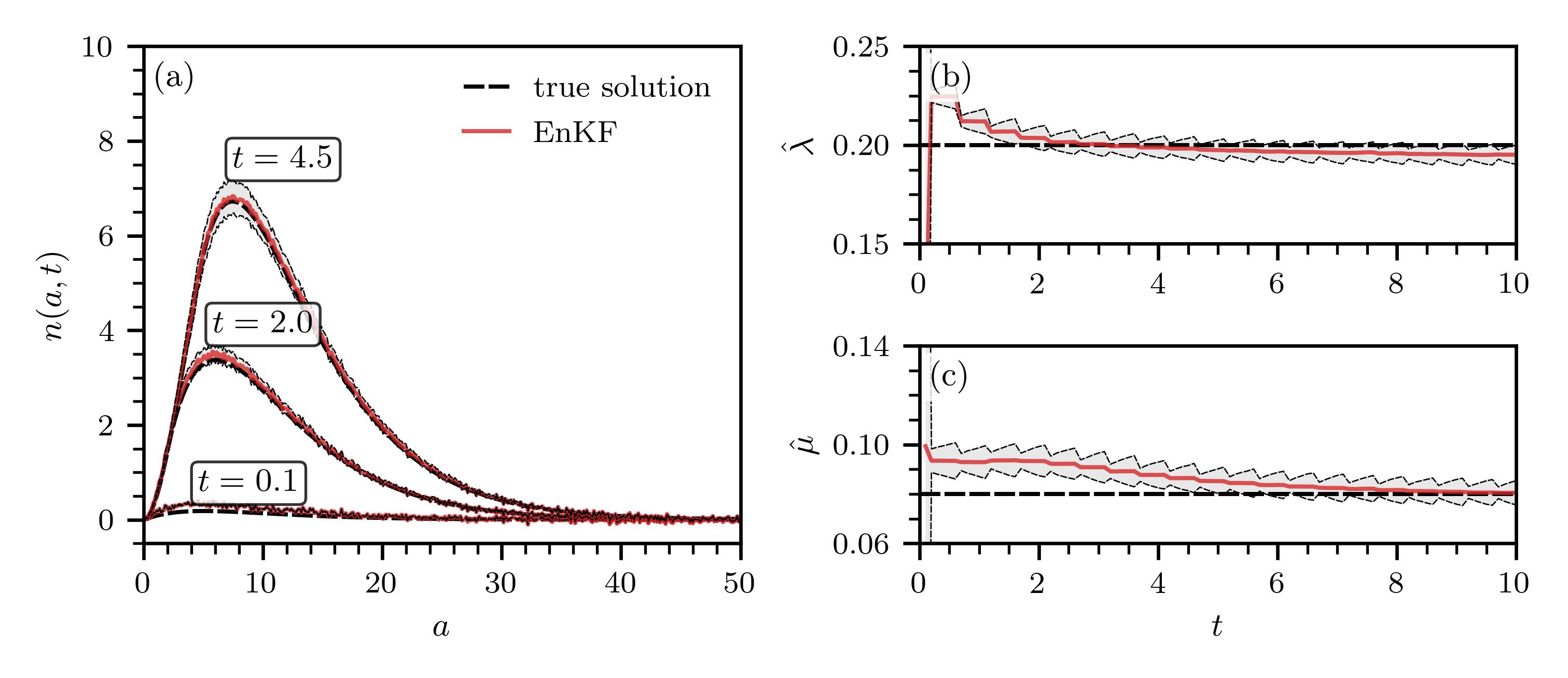
We generate unperturbed observation data from the model using $\mu=0.08/\mathrm{year}$ and $\lambda=0.2/\mathrm{year}$ . The perturbations that we add to $n(a,t)$ are normally distributed with zero mean and variance $10^{-4}$ . Our goal is, given the randomized $n(a,t)$ , to estimate the underlying $\mu$ and $\lambda$ with an EnKF and verify the degree of accuracy of our estimates compared to the original values. In real-world applications, new observation data may not be available for each prediction. To account for this potential lack of observation data, we perform update steps (i.e., integrate observation data into our predictions) every five prediction periods.

Figure 1(a) shows the evolution of both the true solution $n(a,t)$ for which $\mu,\lambda$ are known (dashed black lines) and of the corresponding EnKF estimates that use the augmented state (18). Grey-shaded regions indicate 3 $\sigma$ intervals of the EnKF predictions [see Eq. (12)]. We observe that the EnKF produces estimates of $\lambda$ and $\mu$ that are very close to the true solution after $t\raisebox{-3.69899pt}{~\shortstack{$>$ \\ [-0.07cm] $\sim$}}~2$ years and $t\raisebox{-3.69899pt}{~\shortstack{$>$ \\ [-0.07cm] $\sim$}}~7$ years, respectively.

IV Application to drug-overdoses

We now use an EnKF to combine the model in Eq. (1) with corresponding empirical data taken from the CDC WONDER database. Here different causes of death are classified according to the 10th revision of the International Statistical Classification of Diseases and Related Health Problems (ICD-10). We selected ICD-10 codes T40 (poisoning by narcotics and psychodysleptics) and T43.6 (psychostimulants with abuse potential) and all drug-induced deaths, including unintentional death, suicide, homicide, and death by an undetermined cause. We extracted data for the period 1999 until 2020.

In order to interface drug-overdose data with the analytical setup given in Eq. (1), we identify $n(a,t)\,\mathrm{d}a$ as the number of people with SUD (w.r.t. any drug) of ages between $a$ and $a+\mathrm{d}a$ at time $t$ . We also associate the influx into the SUD population with an addiction rate of the non-SUD population: $r(a,t)[N(a,t)-n(a,t)]$ , where $N(a,t)$ is the overall population density at time $t$ from which we subtract $n(a,t)$ , the density of people with an existing SUD. Finally, the prefactor $r(a,t)$ represents an age- and time-dependent addiction rate, which might be modeled Chou and D’Orsogna 2022 or estimated from additional data such as surveys. Including these elements, the model in Eq. (1) is adapted to

\displaystyle\begin{split}\left[\frac{\partial}{\partial a}+\frac{\partial}{\partial t}\right]n(a,t)=&-\mu(a,t)n(a,t)\\ &+r(a,t)[N(a,t)-n(a,t)]\,.\end{split}

(20)

Equation (20) can be recast in the same form as Eq. (1) via

	$\displaystyle\left[\frac{\partial}{\partial a}+\frac{\partial}{\partial t}\right]n(a,t)=$	$\displaystyle-[\mu(a,t)+r(a,t)]n(a,t)$		(21)
		$\displaystyle+r(a,t)N(a,t)\,.$		(21)

Upon comparing Eq. (21) to Eq. (1) we can identify $\mu(a,t)\to\mu(a,t)+r(a,t)$ and $p(a,t)\to r(a,t)N(a,t)$ , so that the analytical solutions to Eq. (21) can be written through the proper substitutions in Eqs. (2) and (3). Apart from $n(a,t)$ , Eq. (21) contains the functions $N(a,t),r(a,t),\mu(a,t)$ . Here we introduce some possible forms for them, based on available data and realistic assumptions. We begin with the entire population density $N(a,t)$ .

Because of different population-level dynamics such as aging and immigration, the population growth in specific age classes is non-monotonic. In principle, it is possible to use interpolation methods and non-linear functions to construct an age-stratified $N(a,t)$ based on empirical population data that is usually available for 5 or 10-year age windows. However, for the sake of analytical tractability, we will assume an age-independent quantity with $N(t)$ and focus on the more general form $N(a,t)$ in future work. To account for the quasi-linear US population growth in the past two decades, we set

N(t)=N_{0}+\Delta Nt\,,

(22)

where $N_{0}=274.9\times 10^{6}$ and ${\Delta N=2.3\times 10^{6}}$ /year. Figure 2 shows the linear model $N(t)$ and the corresponding population data for the period 2000–2020.

To model $r(a,t)$ , we assume a linear combination of two gamma distributions $f_{1}(a;\alpha_{1},\beta_{1}),f_{2}(a;\alpha_{2},\beta_{2})$ , each peaked at different ages, to describe possible variations in the age dependence of the addiction rate. We do this to account for changes in the prevalence of drug type and societal consumption patterns over the 21 year time frame we examine. The quantities $\alpha_{1},\beta_{1}$ and $\alpha_{2},\beta_{2}$ denote shape and rate parameters of the two distributions $f_{1}$ and $f_{2}$ , respectively. We also assume that $r(a,t)$ does not depend on time and write

r(a,t)\equiv r(a)=\frac{r_{0}}{2}\left[f_{1}(a;\alpha_{1},\beta_{1})+f_{2}(a;\alpha_{2},\beta_{2})\right],

(23)

where $r_{0}$ is a base modulating rate.

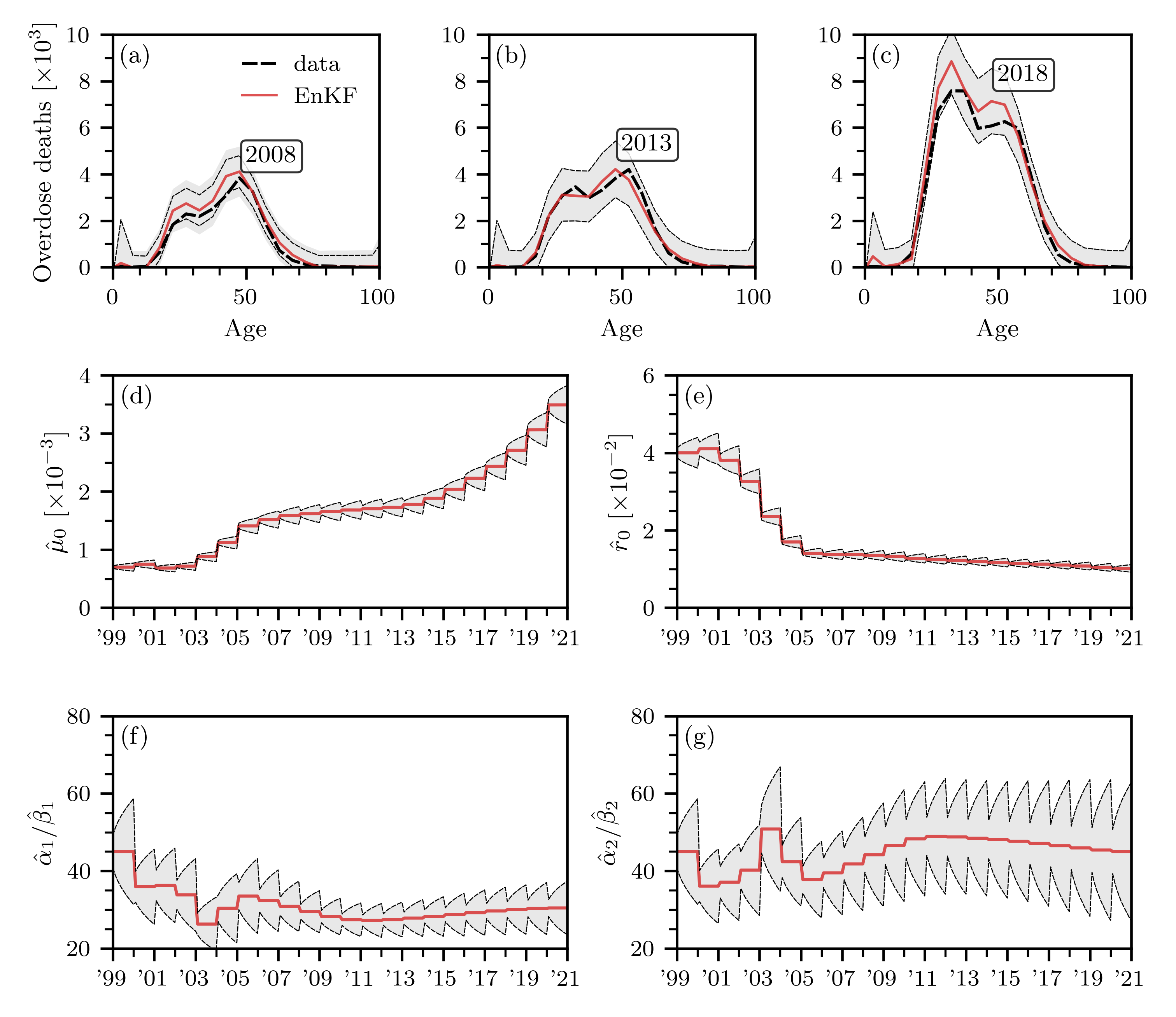
The numerical results that we discuss in the following paragraphs show that a linear combination of two gamma functions allows us to capture the double-peaked distribution of age-stratified overdose deaths [see Fig. 3(a–c)]. Finally, for analytical tractability of the double integrals arising from the solutions of Eq. (21), we retain the constant mortality rate assumption $\mu(a,t)=\mu$ . To combine the mechanistic model in Eq. (21) with empirical data on overdose deaths, we augment the system state $\mathbf{x}(t)$ [see Eq. (8)] by

\begin{split}\tilde{D}(a_{j},t)&=\int_{0}^{t}\mu(a_{j},t^{\prime})n(a_{j},t^{\prime})\,\mathrm{d}t^{\prime}\\ &\hskip 102.43008pt(0\leq j\leq N_{a}-1)\,,\end{split}

(24)

where $\tilde{D}(a_{j},t)$ is the cumulative number of overdose deaths in the age interval $[a_{j},a_{j+1})$ up to time $t$ . We also augment the system state $\mathbf{x}(t)$ by the model parameters $\mu,r_{0},\alpha_{1},\beta_{1},\alpha_{2},\beta_{2}$ that we wish to estimate. As a result, the final augmented system state is

\displaystyle\begin{split}\mathbf{x}(t)=\Big[&n(a_{0},t),\dots,n(a_{N_{a}-1},t),\\ &\hskip 17.07164pt\tilde{D}(a_{0},t),\dots,\tilde{D}(a_{N_{a}-1},t),\\ &\hskip 39.83385pt\mu,r_{0},\alpha_{1},\beta_{1},\alpha_{2},\beta_{2}\Big]^{\top}.\end{split}

(25)

We derive the corresponding rate of change $\mathrm{\partial}n(a,t)/\mathrm{\partial}t$ for the EnKF updates in Appendix A.

For an accurate numerical evaluation of the rate of change of $n(a,t)$ , we use a sufficiently small discretization that is associated with age windows that are more granular than the available overdose data. We thus have to coarse-grain the modeled overdose death densities to be able to relate them to observation data. The CDC WONDER data that we use in this work is based on 22 age groups with $a^{\prime}_{0}=0,a^{\prime}_{22}=120$ years and $\Delta a^{\prime}_{1}=1,\Delta a^{\prime}_{2}=4,\Delta a^{\prime}_{3}=5,\dots,\Delta a^{\prime}_{21}=5,\Delta a^{\prime}_{22}=20$ years. We use a superscript ^′ to distinguish the age discretization in the observation data from the age discretization in the underlying model.

We combine the modeled quantities $\tilde{D}(a_{j},t)$ with corresponding observation data by numerically integrating $\tilde{D}(a_{j},t)$ over age windows $[a^{\prime}_{\ell-1},a^{\prime}_{\ell})$ ( $1\leq\ell\leq 22$ ) to obtain the corresponding number of deaths $D(a^{\prime}_{\ell},t)$ in this age interval at time $t$ . Here, $a^{\prime}_{\ell}=a^{\prime}_{0}+\sum_{m=1}^{\ell}\Delta a_{m}$ for $\ell\geq 1$ . Based on the described mapping of $\tilde{D}(a_{j},t)$ to $D(a^{\prime}_{\ell},t)$ , the measurement function becomes

\mathbf{h}(\mathbf{x}(t))=[D(a^{\prime}_{1},t),D(a^{\prime}_{2},t),\dots]^{\top}\,.

(26)

In our simulations, we set the initial values $n(a_{j},0)=\tilde{D}(a_{j},0)=0$ . The initial values of $\mu$ , $r_{0}$ , $\alpha_{1}$ , $\beta_{1}$ , $\alpha_{2}$ , $\beta_{2}$ are $7\times 10^{-4}\mathrm{/year}$ , $0.04\mathrm{/year}$ , $15$ , $1/(3~\mathrm{year})$ , $15$ , and $1/(3~\mathrm{year})$ , respectively. We have chosen the initial value of $r_{0}$ in accordance with corresponding empirical data on the number of substance initiates Lipari and Park-Lee 2019. The initial mean of both gamma distributions is equal to $\alpha_{1}/\beta_{1}=\alpha_{2}/\beta_{2}=45$ years. To ensure that the parameters $\mu$ , $r_{0}$ , $\alpha_{1}$ , $\beta_{1}$ , $\alpha_{2}$ , $\beta_{2}$ stay positive during EnKF iterations, we use the same exponential transform as in Sec. III.2. All initial covariances are set to $10^{-4}$ , except for the diagonal elements associated with $\mu$ , $r_{0}$ , $\alpha_{1}$ , $\beta_{1}$ , $\alpha_{2}$ , $\beta_{2}$ , which are set to $10^{-2}$ . The process and observation noise covariances are as in Sec. III.2. We use a small process noise and a relatively large initial model parameter variance to (i) let the dynamics evolve according to the mechanistic drug-overdose model without too much additional noise in $n(a,t)$ , $\tilde{D}(a,t)$ and (ii) let the filter explore different trajectories associated with appreciable variations in the underlying model parameters. We have also performed simulations for larger process noise values associated with $n(a,t)$ and $\tilde{D}(a,t)$ . For example, we set the corresponding diagonal elements of $Q$ to values between 1 and 100 without observing substantial differences in the simulation results. In the measurement process, we divide $\tilde{D}(a,t)$ by $10^{3}$ to work with numerical values of $\mathcal{O}(1)$ when comparing predicted and observed overdose fatalities. A measurement variance of $10^{-4}$ (i.e., a standard deviation of $10^{-2}$ ) corresponds to about 10–100 overdose fatalities in the simulated data. Although the exact measurement noise is difficult to estimate given the unknown number of undocumented fatal drug-overdose cases, we used a standard deviation of about 10–100 as a reasonable modeling choice. In our simulations, we use a relatively large ensemble size of $M=10^{4}$ to minimize the effect of sampling errors that occur during the Monte Carlo approximation of the system state evolution in the prediction and update steps. Our simulations start in 1998 and we use a timestep of $\Delta t=0.1$ years.

Figure 3(a–c) shows reported drug-overdose deaths (dashed black lines) for the years 2008, 2013, and 2018. Solid red lines represent EnKF predictions that are based on updates that involved observation data from all previous years since 1999. No additional observation data were available between two subsequent years. That is, for predictions that were made for, e.g., 2008, the most recent observation data that was available to the EnKF was from 2007. Still, the EnKF predictions in Fig. 3(a–c) are closely aligned with the reported overdose deaths. For almost all age classes, predicted overdose fatalities lie within the shown 3 $\sigma$ regions (grey shaded regions). For applications in real-time monitoring of overdose fatalities, one may also include provisional data that becomes available during the course of a year to further refine forecasts.

The evolution of $\hat{\mu}$ and $\hat{r}_{0}$ [see Fig. 3(d,e)] suggests that drug-overdose mortality increased over the years while the proportion of newly addicted individuals approaches about $0.01\mathrm{/year}$ . Up until 2001-2002, the evolution of the mean values of both gamma functions is synchronous [see Fig. 3(f,g)]. From 2003 onwards, one gamma function captures the addiction dynamics of individuals who are older than 40 years, while the second gamma function captures the inflow of younger people with substance use disorder.

Finally, in Fig. 4, we show forecasts of overdose mortality in the US for the years 2021, 2022, and 2023. The latest observation data that is available for these forecasts is from 2020 (dashed black lines in Fig. 4). The predicted overdose mortality in 2021 is slightly smaller than in 2020 in age groups between 30–60. In 2022 and 2023, the predicted overdose mortality in many age groups exceeds that of 2020. Since the overall overdose mortality has increased unsteadily more than five-fold in the past two decades (with a particularly steep increase between 2019 and 2020), the variance in the shown forecasts is relatively large.

V Discussion and Conclusions

We have developed an age-structured model of drug-overdose mortality. Our model accounts for age and time-dependent addiction and mortality rates. It can readily be extended to account for multiple drug classes and different ways of stratifying the population. In a simple example, we have shown how age-structured models can be combined with data-assimilation methods such as an ensemble Kalman filter (EnKF) to forecast the evolution of fatalities and estimate model parameters.

Combining our age-specific overdose model with empirical data on overdose fatalities in the US, we have provided a proof-of-principle set of methods that can be useful for estimating parameters governing drug addiction and mortality and for forecasting the evolution of population-level overdose dynamics.

In addition to developing a framework to include provisional overdose data and retrospective updates of observation data, possible future work includes the study of how regularization terms can help smooth Kalman filter updates Johns and Mandel 2008, or how other ensemble-based Kalman filters, such as ensemble adjustment Kalman filters Anderson 2001, may help improve numerical stability and forecast accuracy. For applications of the proposed methodology to small population sizes, it might be worthwhile to update the age-stratified population using a Poisson-process model, where the Gaussian noise term only affects the underlying model parameters and not the population numbers themselves. Since we focused on drug-overdose forecasting over the past two decades, we decided to use the EnKF in a forward mode and not use backward passes/smoothing (i.e., not use future observations from times $t^{\prime}>t$ at time $t$ ). As noted by Evensen and van Leeuwen Evensen and Van Leeuwen 2000, in forecasting mode, the EnKF and ensemble Kalman smoother (EnKS) produce the same state estimate at the latest time. However, using backward passes and an EnKS (or lagged versions) can help improve earlier parameter estimates, which is also an interesting direction for future research. Another possible direction for future work is to extend the presented data assimilation framework to account for age-dependent death rates $\mu(a,t)$ and age-dependent population data $N(a,t)$ in Eq. (21).

Declarations

•

Funding: We acknowledge financial support from the ARO through grant W911NF-18-1-0345 (M.R.D and T.C.), the NIH through grant R01HL146552 (T.C.), and the NSF through grant DMS-1814090 (M.R.D.).
•

Conflict of interest/Competing interests: The authors declare no competing interests.
•

Availability of data and materials: All mortality datasets are publicly available at https://gitlab.com/ComputationalScience/overdose-da and at https://wonder.cdc.gov/mcd.html.
•

Code availability: All source codes are publicly available at https://gitlab.com/ComputationalScience/overdose-da.
•

Authors’ contributions: All authors contributed equally.

Appendix A Rate of change

We evaluate the derivative of Eq. (2) w.r.t. $t$ for $t_{0}=0$ , $r(a,t)\equiv r(a)=r_{0}\left[f_{1}(a;\alpha_{1},\beta_{1})+f_{2}(a;\alpha_{2},\beta_{2})\right]/2$ , $N(t)=N_{0}+\Delta Nt$ , $\mu(a,t)=\mu$ . The resulting rate of change of $n(a,t)$ for $a>t$ is

	$\displaystyle\frac{\partial n(a,t)}{\partial t}=$	$\displaystyle-\big[\rho^{\prime}(a-t)+\rho(a-t)(\mu+r(a-t))\big]e^{-\mu t-\int_{0}^{t}r(a-t+s)\,\mathrm{d}s}+r(a)N(t)$		(27)
		$\displaystyle-\int_{0}^{t}e^{-\mu(t-s)-\int_{s}^{t}r(a-t+s^{\prime})\,\mathrm{d}s^{\prime}}N(s)\Big(r(a-t+s)\big(\mu+r(a-t+s)\big)+r^{\prime}(a-t+s)\Big)\,\mathrm{d}s.$		(27)

For $a<t$ , the rate of change is

\displaystyle\frac{\partial n(a,t)}{\partial t}=\int_{0}^{a}\!r(s)\Delta Ne^{-\mu(a-s)-\int_{s}^{a}r(s^{\prime})\,\mathrm{d}s^{\prime}}\,\mathrm{d}s\,.

(28)

The integrals $\int_{s}^{t}r(a-t+s^{\prime})\,\mathrm{d}s^{\prime}$ , $\int_{0}^{t}r(a-t+s)\,\mathrm{d}s$ , and $\int_{s}^{a}r(s^{\prime})\,\mathrm{d}s^{\prime}$ can be evaluated using the identity

\int_{s}^{t}\frac{\beta^{\alpha}}{\Gamma(\alpha)}(a-t+s^{\prime})^{\alpha-1}e^{-\beta(a-t+s^{\prime})}\,\mathrm{d}s^{\prime}=\frac{1}{\Gamma(\alpha)}\left[\Gamma(\alpha,(a-t+s)\beta)-\Gamma(\alpha,a\beta)\right],

(29)

where $\Gamma(s,x)=\int_{x}^{\infty}t^{s-1}e^{-t}\,\mathrm{d}t$ denotes the upper incomplete gamma function. We evaluate the remaining integrals $\int_{0}^{t}(\cdot)\,\mathrm{d}s$ numerically. The simulation results that we present in Sec. IV use the age-dependent initial condition

\rho(a)=0.04N_{0}f(a;\alpha,\beta)\,,

(30)

where $f(a;\alpha,\beta)$ is a gamma distribution with shape and rate parameters $\alpha$ and $\beta$ , respectively. In all simulations, we set $\alpha=15$ and $\beta=1/(3~\mathrm{year})$ such that the distribution mean is 45 years. The prefactor of 0.04 is chosen such that initially 4% of the population are suffering from a substance use disorder Lipari and Park-Lee 2019.

References

Jalal et al. (2018) H. Jalal, J. M. Buchanich, M. S. Roberts, L. C. Balmert, K. Zhang, and D. S. Burke, Changing dynamics of the drug overdose epidemic in the United States from 1979 through 2016, Science 361, eaau1184 (2018).
Jalal et al. (2020) H. Jalal, J. M. Buchanich, D. R. Sinclair, M. S. Roberts, and D. S. Burke, Age and generational patterns of overdose death risk from opioids and other drugs, Nat. Med. 26, 699 (2020).
Ahmad et al. (2021) F. B. Ahmad, L. M. Rossen, and P. Sutton, Provisional drug overdose death counts (2021).
D’Orsogna et al. (2023) M. R. D’Orsogna, L. Böttcher, and T. Chou, Fentanyl-driven acceleration of racial, gender and geographical disparities in drug overdose deaths in the United States, PLOS Glob. Public Health 3, e0000769 (2023).
M’Kendrick (1925) A. M’Kendrick, Applications of Mathematics to Medical Problems, Proc. Edinb. Math. Soc. 44, 98 (1925).
Chou and Greenman (2016) T. Chou and C. D. Greenman, A hierarchical kinetic theory of birth, death and fission in age-structured interacting populations, J. Stat. Phys. 164, 49 (2016).
Evensen (1994) G. Evensen, Sequential data assimilation with a nonlinear quasi-geostrophic model using Monte Carlo methods to forecast error statistics, J. Geophys. Res. Oceans 99, 10143 (1994).
Crassidis and Junkins (2004) J. L. Crassidis and J. L. Junkins, Optimal estimation of dynamic systems (Chapman and Hall/CRC, Boca Raton, FL, 2004).
Brown and Hwang (2012) R. G. Brown and P. Y. Hwang, Introduction to random signals and applied Kalman filtering: with MATLAB exercises and solutions (Wiley, Hoboken, NJ, 2012).
Fang et al. (2015a) B. Fang, X.-Z. Li, M. Martcheva, and L.-M. Cai, Global asymptotic properties of a heroin epidemic model with treat-age, Appl. Math. Comput. 263, 315 (2015a).
Fang et al. (2015b) B. Fang, X. Li, M. Martcheva, and L. Cai, Global stability for a heroin model with age-dependent susceptibility, J. Syst. Sci. Complex. 28, 1243 (2015b).
Yang et al. (2016) J. Yang, X. Li, and F. Zhang, Global dynamics of a heroin epidemic model with age structure and nonlinear incidence, Int. J. Biomath. 9, 1650033 (2016).
Liu and Liu (2019) L. Liu and X. Liu, Mathematical analysis for an age-structured heroin epidemic model, Acta Appl. Math. 164, 193 (2019).
Chekroun et al. (2020) A. Chekroun, M. N. Frioui, T. Kuniya, and T. M. Touaoula, Mathematical analysis of an age structured heroin-cocaine epidemic model, Discrete Contin. Dyn. Syst. - B 25, 4449 (2020).
Din and Li (2020) A. Din and N. Li, Controlling heroin addiction via age-structured modeling, Adv. Differ. Equ. 521 (2020).
Duan et al. (2021) X. Duan, H. Cheng, M. Martcheva, and S. Yuan, Dynamics of an age structured heroin transmission model with imperfect vaccination, Int. J. Bifurc. Chaos 31, 2150157 (2021).
Khan et al. (2021) A. Khan, G. Zaman, R. Ullah, and N. Naveed, Optimal control strategies for a heroin epidemic model with age-dependent susceptibility and recovery-age, AIMS Math. 6, 1377 (2021).
Bélair et al. (1995) J. Bélair, M. C. Mackey, and J. M. Mahaffy, Age-structured and two-delay models for erythropoiesis, Math. Biosci. 128, 317 (1995).
Mahaffy et al. (1998) J. M. Mahaffy, J. Bélair, and M. C. Mackey, Hematopoietic model with moving boundary condition and state dependent delay: applications in erythropoiesis, J. Theor. Biol. 190, 135 (1998).
Chuang et al. (2018) Y.-L. Chuang, T. Chou, and M. R. D’Orsogna, Age-structured social interactions enhance radicalization, J. Math. Sociol. 42, 128 (2018).
Wang et al. (2022) Y. Wang, R. Dessalles, and T. Chou, Modeling the impact of birth control policies on China’s population and age: effects of delayed births and minimum birth age constraints, R. Soc. Open Sci. 9, 211619 (2022).
Böttcher et al. (2020) L. Böttcher, M. Xia, and T. Chou, Why case fatality ratios can be misleading: individual-and population-based mortality estimates and factors influencing them, Phys. Biol. 17, 065003 (2020).
Richard et al. (2021) Q. Richard, S. Alizon, M. Choisy, M. T. Sofonea, and R. Djidjou-Demasse, Age-structured non-pharmaceutical interventions for optimal control of COVID-19 epidemic, PLOS Comp. Biol. 17, e1008776 (2021).
Kreck and Scholz (2022) M. Kreck and E. Scholz, Back to the roots: A discrete Kermack–Mckendrick model adapted to Covid-19, Bull. Math. Biol. 84, 1 (2022).
Katzfuss et al. (2016) M. Katzfuss, J. R. Stroud, and C. K. Wikle, Understanding the ensemble Kalman filter, Am. Stat. 70, 350 (2016).
Lillacci and Khammash (2010) G. Lillacci and M. Khammash, Parameter estimation and model selection in computational biology, PLOS Comp. Biol. 6, e1000696 (2010).
Pandey et al. (2013) A. Pandey, A. Mubayi, and J. Medlock, Comparing vector–host and SIR models for dengue transmission, Math. Biosci. 246, 252 (2013).
Bomfim et al. (2020) R. Bomfim, S. Pei, J. Shaman, T. Yamana, H. A. Makse, J. S. Andrade Jr, A. S. Lima Neto, and V. Furtado, Predicting dengue outbreaks at neighbourhood level using human mobility in urban areas, J. R. Soc. Interface 17, 20200691 (2020).
Reis et al. (2022) S. D. Reis, L. Böttcher, J. P. d. C. Nogueira, G. S. Sousa, A. S. L. Neto, H. J. Herrmann, and J. S. Andrade Jr, Spatio-temporal characteristics of dengue outbreaks, Front. Phys. 10, 923099 (2022).
Pei et al. (2021) S. Pei, F. Liljeros, and J. Shaman, Identifying asymptomatic spreaders of antimicrobial-resistant pathogens in hospital settings, Proc. Natl. Acad. Sci. U.S.A. 118, e2111190118 (2021).
Schneider et al. (2022) T. Schneider, O. R. Dunbar, J. Wu, L. Böttcher, D. Burov, A. Garbuno-Iñigo, G. L. Wagner, S. Pei, C. Daraio, R. Ferrari, et al., Epidemic management and control through risk-dependent individual contact interventions, PLOS Comp. Biol. (2022).
Böttcher and Gersbach (2020) L. Böttcher and H. Gersbach, The great divide: drivers of polarization in the US public, EPJ Data Sci. 9, 1 (2020).
Lipari and Park-Lee (2019) R. N. Lipari and E. Park-Lee, Mental Health Services Administration. Key substance use and mental health indicators in the United States: Results from the 2018 National Survey on Drug Use and Health (HHS Publication No. PEP19-5068, NSDUH Series H-54). Rockville, MD: Center for Behavioral Health Statistics and Quality, Substance Abuse and Mental Health Services Administration (2019).
Labbe (2022) R. Labbe, Kalman and Bayesian Filters in Python, https://github.com/rlabbe/Kalman-and-Bayesian-Filters-in-Python/blob/master/Appendix-E-Ensemble-Kalman-Filters.ipynb (2022).
Chou and D’Orsogna (2022) T. Chou and M. D’Orsogna, A mathematical model of reward-mediated learning in drug addiction, Chaos 32, 021102 (2022).
Johns and Mandel (2008) C. J. Johns and J. Mandel, A two-stage ensemble Kalman filter for smooth data assimilation, Environ. Ecol. Stat. 15, 101 (2008).
Anderson (2001) J. L. Anderson, An ensemble adjustment Kalman filter for data assimilation, Mon. Weather Rev. 129, 2884 (2001).
Evensen and Van Leeuwen (2000) G. Evensen and P. J. Van Leeuwen, An ensemble Kalman smoother for nonlinear dynamics, Mon. Weather Rev. 128, 1852 (2000).