Reactive Gait Composition with Stability: Dynamic Walking amidst Static and Moving Obstacles
Abstract
This paper presents a modular approach to motion planning with provable stability guarantees for robots that move through changing environments via periodic locomotion behaviors. We focus on dynamic walkers as a paradigm for such systems, although the tools developed in this paper can be used to support general compositional approaches to robot motion planning with Dynamic Movement Primitives (DMPs). Our approach ensures a priori that the suggested plan can be stably executed. This is achieved by formulating the planning process as a Switching System with Multiple Equilibria (SSME) and proving that the system’s evolution remains within explicitly characterized trapping regions in the state space under suitable constraints on the frequency of switching among the DMPs. These conditions effectively encapsulate the low-level stability limitations in a form that can be easily communicated to the planner to guarantee that the suggested plan is compatible with the robot’s dynamics. Furthermore, we show how the available primitives can be safely composed online in a receding horizon manner to enable the robot to react to moving obstacles. The proposed framework is applied on 3D bipedal walking models under common modeling assumptions, and offers a modular approach towards stably integrating readily available low-level locomotion control and high-level planning methods.
I Introduction
The ability to navigate in changing environments is central to developing autonomous robots. Many approaches aim at enabling robots to “translate” a navigation task to a sequence of motion (or, movement) primitives, the execution of which transfers a robot to a desired location, avoiding obstacles on the way. These approaches lend themselves naturally to a hierarchical formulation, wherein, at the high level, the requisite primitive sequence is constructed, and then realized at the low level via suitable feedback control laws. One important advantage of this hierarchy is that the low-level control and high-level planning modules can be treated separately. This benefit, however, comes with the challenge of ensuring safe integration of the control and planning modules; here, the term “safe” incorporates both collision-free navigation and stable platform operation.
I-A Central themes and relation to prior work
This paper proposes and rigorously analyzes, a modular framework (Fig. 1), within which established planning and control design methods can be integrated in a provably stable way. We focus on robots that move through their environment via dynamic rhythmic interactions, adopting dynamically stable walking bipeds [1, 2, 3] as an example. However, the tools developed in this paper can, in principle, be used to safely plan motions for aerial [4] and underwater [5] vehicles that use oscillating appendages—e.g., flapping wings or flippers—for locomotion.
At the core of our approach is the notion of a DMP (DMP) [6], which in the case of dynamic walkers takes the form of a stride-to-stride map with a locally asymptotically stable fixed point representing a desired periodic locomotion behavior (Fig. 1). Thus, a DMP captures the local dynamics around a nominal locomotion behavior at the stride level. Execution of each DMP results in a displacement in the robot’s workspace; these displacements form actions available for planning (Fig. 1). To derive conditions under which the planner’s suggestions are compatible with the platform’s stability limitations, this paper formulates the planning process as a SSME (SSME) in discrete time (Fig. 1), and proves that its solution can be confined in an explicitly characterized safe region provided that a bound on the frequency of DMP switching is imposed. This bound effectively compresses the information relevant to stable switching of DMPs to a single number, which can be easily communicated to the planner. Besides stability, these results enable the effective approximation of the DMPs in a form that reduces computational effort, allowing online locomotion planning in the presence of moving obstacles.
This paper extends our preliminary work [7, 8] in three directions. First, it characterizes the dynamic properties of 3D bipeds that enable the application of the proposed approach. Second, it applies the notion of practical stability [9, p. 121] and recent theoretical developments in SSMEs [10] to derive explicit conditions for stable reactive planning with dynamic walking gaits. Third, it demonstrates how the a priori known stability conditions can be exploited to formulate a primitive-based sequential MPC (MPC) scheme for online planning that allows dynamically walking bipeds to react to moving obstacles.


I-B Related work
This section surveys related work and highlights connections and contributions to these approaches.
I-B1 Locomotion as a limit cycle
Dynamically stable walking is characterized by alternating phases of fall-and-capture pendular motions [1, 2]. Stability in this case is often evaluated by treating the gait as a whole [3], and can be captured by the stability properties of isolated periodic solutions—i.e., limit cycles—in the system’s state space [11]. A significant volume of research on dynamically stable bipeds revolves around low-level feedback control design methods for walking or running motions; the book [12] contains several approaches. An example is the HZD (HZD) method [11] and its extensions [13, 14, 15, 16, 17]; see [18] for an overview. Typically, however, control design methods for dynamically stable walking do not consider high-level planning objectives, such as avoiding unsafe regions on the walking surface or in the robot’s workspace. Notable exceptions include [19], which uses an energy-based planner to output suitable sequences of virtual constraints that generate feasible walking on known uneven terrain, and [20, 21] where one- or two-step nominally periodic gaits are safely “deformed” to comply with precise foot positioning specifications. Most relevant to our work are [22, 23] which use a library of limit-cycle walking gaits to generate collision-free paths in spaces cluttered by static obstacles.
In this paper, we interpret limit cycles as task-simplifying locomotion abstractions [24] that generate suitable actions available for high-level planning. Formally, these abstractions take the form of pairs of stride-to-stride maps together with locally asymptotically stable fixed points as in [22, 23], and thus can be considered as discrete-time versions of DMPs [6].
I-B2 Switched systems and motion planning
Planning motions via DMPs can be formulated as a switched dynamical system. The earliest work that makes this connection explicit in the context of dynamically walking bipeds is [22, 23], which also discusses the existence of a bound on the frequency of switching that ensures stability of the resulting walking sequence. However, this bound is estimated on the basis of computationally intensive simulations. The relation between switching frequency and stability is prevalent in the theory of switched systems, and can be captured by the notion of dwell time, which was introduced in [25] for switching among dynamical systems that share a common equilibrium; refer to [26] for a thorough study. Contrary to that work, switched systems formulations of motion planning problems are characterized by switching among systems with distinct equilibria. An early study of such systems can be found in [27], which established boundedness of solutions under a fixed dwell-time bound. This bound was adapted to switched discrete-time systems in our previous work [7], where it was applied to bipedal robot navigation amidst static obstacles. Beyond obstacle avoidance, switching11 1 Related to gait switching is gait interpolation, which has been used in [28, 29] to track a speed profile, in [30] to walk on stochastic terrain, and in [31] to plan motions in height-constraint environments. has been used to realize robust walking on uneven terrain with varying slope [32] or height [33, 19, 34], and to achieve gait adaptation under persistent external forcing [35, 36, 37] and model uncertainty [38]. Switching has also been used to create hopping motions with speed adaptation in monopods [39, 40], and to study gait transitions in quadrupeds [41, 42, 43].
This paper takes advantage of recent theoretical tools for SSMEs [36, 44, 10] to contribute to switching approaches for motion planning an explicit set characterization for practically stable DMP composition in a model predictive fashion. This way, changes in the robot’s workspace during plan execution, such as moving obstacles, can be taken into account. These tools are relevant to other robots, which—like legged robots–move via periodic interactions; e.g., aerial robots with flapping wings [45, 4], and underwater robots with paddles [5].
I-B3 Compositional approaches to planning
The DMPs defined in this paper correspond to attractive “landscapes” in the state space, focused at asymptotically stable equilibrium behaviors. In our discrete-time setting [7], certificates for asymptotically stable equilibria can be obtained by discrete-time Lyapunov functions [46, Chapter 13], which can be idealized as ‘‘funnels’’ attracting the (discrete-time) flow of the system towards their center. This idealization was made explicit22 2 As stated in [47], the notion of a funnel was first proposed as a metaphor for robust behaviors in [48] and sequential composition was introduced in [49] to combine controllers via pre-image backchaining from the overall task goal in the context of fine-motion planning. in [47], where funnels were sequentially composed to generate dexterous “batting” maneuvers in a robot arm. Taking advantage of breakthrough developments in the automatic verification of Lyapunov functions using SOS (SOS) programming [50] and in sample-based randomized motion planning algorithms [51], LQR trees have been introduced in [52] as a computationally tractable approach to feedback motion planning for nonlinear systems. However, LQR trees cannot address situations in which the environment is only partially known prior to runtime; online implementation of the algorithm to handle changing environments is computationally infeasible [53]. To compose plans under uncertainty at runtime, [53] introduced a funnel library and applied the method to a small airplane performing obstacle avoidance tasks.
Infinite-horizon Lyapunov funnels, such as those employed in [47] and in our prior work [7], represent convenient ways to describe positively invariant sets; thus, composition of Lyapunov funnels is related to motion planning with positively invariant set trees [54, 55]. These algorithms construct a tree of local state feedback control laws, each stabilizing a randomly sampled equilibrium, and use the corresponding positively invariant sets to decide when to safely transition from one controller to another. As in LQR trees, invariant set trees are extended backwards from the goal until they contain the initial condition, and thus they are not directly suited to receding-horizon problems [56].
To achieve reactivity to changes in the environment, recent methods integrate a dedicated high-level component in the planning and control hierarchy. In [57], this component relies on behavior trees to achieve efficient re-planning in changing environments. Another example of a hierarchical planning and control architecture can be found in [58], wherein a deliberative layer suggests a sequence of parameterized actions for a given task, a reactive layer converts these actions to target velocity commands, and a gait layer realizes those commands on the robot. Finally, [59] proposes a reactive high-level planner based on Linear Temporal Logic; the suggested plans are then translated to robot motions using a reduced-order model ensuring safety within the context of that model.
I-B4 Reduced-order bipedal locomotion models
Given the high-dimensional, nonlinear dynamics of bipedal walkers, several planning methods rely on reduced-order models [60, 61] to resolve complexity. Prominent among these models is the LIP (LIP) [62]. However, establishing a formal connection between a reduced-order model selected a priori and the full-order dynamics of the system remains largely an open problem. An early result in that direction can be found in [63] where a SLIP (SLIP) is embedded as the HZD of an asymmetric hopper so that solutions of the (pre-selected) reduced-order model are also solutions of the closed-loop full dynamics. However, selecting the target reduced-order model in advance and establishing the geometric constructions required in [63] can be overly restrictive [64]. A less strict form of correspondence was recently proposed in [65] where an approximate simulation relation between a LIP and a 30 DOF (DOF) model of the Valkyrie humanoid was established.
An alternative approach—and the one we adopt in this paper—is to refrain from selecting in advance the reduced-order model used for planning. Instead, we start with the full-order system and impose virtual constraints to reduce it to a lower dimensional subsystem, which is not specified a priori and can be used to define reduced-order DMPs. Combining this reduction approach with the explicit characterization of solution trapping regions is the key to efficient computation via approximate planning actions.
Notation
and represent real and integer numbers, while and denote their non-negative counterparts. The index represents discrete time. Norms are denoted by . If , denotes the interior of . We use for the special orthogonal group of dimension and to denote the unit circle. A continuous function is of class if it is strictly increasing, and [46, p. 162].
II Overview: Planning with DMPs
This section provides an overview of our approach—see also Fig. 1—and serves as a guide for the rest of the paper; technical details are left to subsequent sections.
II-A Problem formulation: Planning with limit cycles
We consider a class of locomotion systems evolving in spaces that can be decomposed into a global position and heading part and a state part . It is assumed that contains distinguished periodic orbits—i.e., limit cycles—corresponding to gaits of interest. Suppose that is a limit cycle corresponding to one such gait (see Fig. 1), and let be a surface transversal to . Then, can be represented by a fixed point of the discrete-time system
| (1) |
where is the corresponding Poincaré map and . Intuitively, (1) captures the discrete evolution of successive crossings through the surface . As the state evolves on according to (1), the pose—that is, the location and heading—of the system in is also updated in a discrete fashion. Given a coordinate representation , this discrete update can be captured by the displacement map so that
| (2) |
Combining (1) and (2), we define the (augmented) stride map by
| (3) |
that captures the complete stride-to-stride evolution.
Owing to the structure of (3), planning can be naturally decomposed in a low-level gait generation problem governed by the state and its evolution on according to (1), and a high-level planning problem in captured by the displacement map (see Figs. 1-1). Consider now a system for which a finite number of limit-cycle gaits , , is available. The dynamics around each limit cycle is represented by a pair
| (4) |
where is the corresponding Poincaré map and . We require that, for each , is a locally exponentially stable fixed point of the corresponding map33 3 For systems with impulse effects such as the ones arising in legged locomotion, [66, Corollary 1] establishes that is a locally exponentially stable limit cycle if, and only if, is a locally exponentially stable equilibrium of the corresponding map . More details on this can be found in [66, 67]; we will not delve deeper into this matter here, focusing on the stride-to-stride evolution of the system. . Thus, we adopt a dynamical systems perspective to planning robot motions, according to which primitive movements are represented by (discrete-time) attractor landscapes , as in [6]. We refer to these DMPs as gait primitives, and to the collection as the gait library.
Suppose now that a gait library is available. The execution of each primitive in results in displacement of the robot in according to (2). Thus, for each , augmenting the gait primitives in (4) with the corresponding displacements provides actions
| (5) |
available for planning; see Figs. 1–1. Note that each action (5) represents a prediction. That is, if is the state at the beginning of a stride, predicts the displacement and the state update caused if the gait primitive is engaged in the forthcoming stride. The predicted state is then used to evaluate the displacements available to the planner at the next stride and so on.
This paper focuses on navigation problems, wherein a robot is tasked with reaching a target location in its workspace that contains both static and moving obstacles. To achieve this, a planning algorithm equipped with a collection of actions is used to find a sequence that maps the stride number to the index
| (6) |
of the action required at that stride. The suggested sequence of actions is then realized by concatenating the corresponding gait primitives (4) according to (6).
II-B Challenges and contributions
Before continuing, it is important to identify the main challenges of the approach described above.
II-B1 Symmetry properties and model structure
Our approach exploits the “triangular” (cf. [68, p. 43]) structure of the augmented stride map (3) to separate gait generation from navigation. Implicit in (3) is the assumption that the stride-to-stride evolution of the system’s state and the net change of the pose of the system in given by (1) and (2) respectively, do not depend on the system’s pose at the beginning of the stride. In Section III we show that under mild assumptions, a large class of 3D bipedal walking models possesses augmented stride maps that have the structure of (3).
II-B2 Practically stable path planning
The realization of the sequence of actions according to (6) requires the implementation of the corresponding gait primitives . However, this sequence of gaits may result in loss of stability, even when each gait primitive is itself stable. Defining what stability means in our setting is challenging; for, switching due to planning commands causes the system to be in an “unrelenting” transient phase, never converging to any of the underlying equilibrium behaviors. Beyond analysis, it is also important to be able to communicate stability constraints to the planner so that the suggested plans are compatible with stable operation. These issues are addressed in Section IV, where the set-based notion of practical stability is adopted to identify a class of switching signals that provably guarantee stable operation as the system switches among the primitives in . These signals are characterized by a lower bound on the dwell time between switches. This way, the information relevant to stability is “compressed” to a single number or pair of numbers, which can be easily communicated to the planner.
II-B3 Reactive path planning and computational tractability
While feasible offline, the need to resort to numerical integration to evaluate the maps and challenges the implementation of optimization-based path planning approaches in real time. To enable computationally efficient implementation, Section V below provides a method for extracting a collection , of approximate actions, represented as closed-form estimates of the maps and in (5). This way, the planner has the ability to (approximately) predict the future stride-to-stride evolution of the system, and use this information to adjust its actions online while being consistent with practically stable gait switching without adversely affecting computational time. This is achieved in a primitive-based MPC fashion in Section VI.
III 3D Bipedal Walking Models: Main Properties
This section identifies a general class of 3D walking robot models and feedback control laws that result in the “triangular” structure (3) of the corresponding stride-to-stride map. Our discussion here is not restricted to a particular robot model or controller structure; rather, the focus is on the properties that enable the decomposition of the planning problem to task-relevant and gait-design components, as described in Section II-A.
III-A Dynamics: Symmetry properties
Bipedal robot models can be represented as tree structures of rigid bodies; see Fig. 1. We will assume that each joint is revolute and allows a single DOF rotation; note that this assumption does not entail significant loss of generality since multi-DOF joints—e.g., ball joints—can be represented by multiple single-DOF revolute joints with links of zero length in between [69]. Let be an inertia frame with its -axis aligned with the direction of gravity and the -axis and -axis forming a plane that represents the ground surface. It is assumed here that the ground is flat and not deformable. Let and be the position and orientation with respect to of a body-fixed frame attached at a reference (base) link. If includes the relative angles of the rest of the links that determine the shape of the multi-body chain, the configuration of the floating-base model can be captured by . Choosing a minimal representation of by the yaw , pitch , and roll angles, we use to describe the angular configuration of the model in a subset of that contains physically reasonable configurations.
Bipedal walking is composed by alternating single and double support phases. In single support—left or right—we assume that the foot in contact with the ground remains stationary. Then, attaching at the support foot implies . Without loss of generality, we can take and identify with its non-zero components; thus, with a slight abuse of notation, . During the single support phase, neither the kinetic nor the potential energy depend on the location with respect to . Hence, if is the corresponding Lagrangian, the equations of motion can be written as
| (7) |
where are the generalized forces due to the motor torques .
The continuous-time evolution of single support is interrupted when the swing leg contacts the ground. This event occurs when the vertical distance of the tip of the swing leg from the ground reduces to zero. Due to the flat ground assumption, this distance does not depend on the position of the biped relative to . Hence, if is the map that associates to a configuration the vertical distance of the tip of the swing leg from the ground, contact can be captured by the switching surface
| (8) |
Crossing triggers the double support phase, which is assumed to be instantaneous, and, as a result, can be modeled via a reset map defined on by its components
| (9) |
where are the angles and velocities prior to impact and are the corresponding values after impact. Due to the flat, non-deformable ground, (9) does not depend on the location with respect to ; see [70, 69] for details.
For motion planning, we define the augmented state
| (10) |
where and . In this setting, the dynamics of the system can be written as
| (11) |
where the first two components of the vectors fields and are zero by the fact that and the rest are computed by (7). The augmented switching surface and the augmented reset map can be analogously defined. Collecting all terms, the dynamics of the model can be written as a hybrid system
| (12) |
We are now ready to state properties of (12) that lead to the triangular structure of the augmented stride map (3). First, note that the domain in (12) is decomposed in two parts: (i) the “task-relevant” (planning) part parametrized by the location of the robot and its heading , and (ii) the “gait” part parametrized by the states in (10); that is, as in Section II-A. Next, we examine the effect on (12) of translations along the -axes and rotations about the -axis of . Consider an element of corresponding to a translation by and a rotation by , and let be the map
| (13) |
The following proposition summarizes the properties of the dynamics (12) that are of interest to motion planning.
Proposition 1.
III-B Control: Symmetry-preserving feedback laws
We will be concerned with locomotion control laws that preserve the symmetry properties listed in Proposition 1. To be specific, consider a feedback law that prescribes the actuator inputs during the single support phase by the rule . Let be the solution with initial condition of (11) in closed loop with , i.e.,
| (14) |
where . We then require that is designed so that satisfies the following property
| (15) |
which essentially extends the equivariance property of Proposition 1(i) to the closed-loop system. It is emphasized here that while the properties listed in Proposition 1 are inherent to the class of bipedal robot models described in Section III-A, property (15) hinges upon the design of the feedback controller . This, in turn, depends on the actuation structure in (7), and thus, the design of a controller to satisfy (15) must be grounded to the morphology of the robot; as an example, Section V below examines a common underactuated configuration, in which (15) is naturally satisfied.
III-C The augmented stride map
A full stride consists of right and left single support phases, each having the form of (12). Due to the nontrivial hip width, the equations for right and left support differ, and will be distinguished by the indices and , respectively. If and are feedback control laws designed so that property (15) is satisfied, the resulting closed-loop hybrid system is composed by the right and left support phases and respectively, where and represent the corresponding closed-loop vector fields (14).
To derive the augmented stride map, suppose that is a state that results in a complete stride and let be the initial condition for the ensuing left support phase and be the corresponding flow associated with the closed-loop dynamics . If is the time-to-impact, defined by is the map taking the state prior to left support to the state prior to right support. The map can be defined analogously, and the (full) stride map is44 4 A map can be defined similarly. This map is diffeomorphic to , thus the choice between or is arbitrary; in what follows, we use by (16).
| (16) |
A direct consequence of Proposition 1 and property (15) is that (16) is equivariant under the action defined by (13).
Proposition 2.
A proof of Proposition 2 can be found in Appendix A. Intuitively, (17) implies that rotating with respect to and translating along after completing a stride results in the same displacement as first rotating and translating the robot and then taking a stride.
Property (17) results in the “triangular” structure (3) of . Indeed, let and , where is the switching surface (8) for the right support phase. Then, for , we have
resulting in the augmented stride map (3), where is defined by the first three components of and includes the rest of the components of . As was discussed in Section II-A, the triangular structure (3) of leads to a natural decomposition of the problem to a low-level gait generation component governed by the stride-by-stride update of the state according to , and a high-level planning problem in captured by ; see Fig. 1.
IV Practically Stable Gait Composition
Suppose now that a collection of gait primitives and corresponding actions are available to a planner. To keep the discussion general, we defer the details on how the gait primitives and the corresponding actions are designed to the following section. The task of the planner is to suggest a sequence mapping the current stride number to the index of the gait primitive that must be engaged at that stride so that a higher-level objective is achieved. Implementing the suggested sequence of actions naturally gives rise to a switching system with multiple equilibria
| (18) |
This system differs from classical switching systems—such as those studied in [26] and in references therein—in a fundamental way: the maps do not share the same fixed point; that is, when . In this section, we discuss a theoretical result on the stability properties of systems like (18) that is important in motion planning.
IV-A Preliminaries and definitions
As was mentioned in Section II-B, defining stability in switching systems with multiple equilibria can be challenging; for, continuing switching in response to varying operation conditions causes the system to shift to different equilibria, never converging to any one of them. To certify stability in (18), we will adopt the notion of practical stability, which is defined as follows.
Definition 1 (Adapted from [71]).
Let and be given sets with being closed and bounded and . The switched system (18) is practically stable with respect to and , if implies for all .
In what follows, we will provide explicitly computable characterizations of the sets and for (18) under suitable conditions on the individual gait primitives in and on the switching signal . We begin with the requirement that each gait primitive is locally exponentially stable. Safety certificates of this form can be obtained through suitable Lyapunov functions [46, Chapter 13] defined as follows.
Definition 2.
Consider the discrete-time system (1) defined on . Let be an open subset of with . A continuous function is an exponential Lyapunov function, if, for all ,
| (19) |
| (20) |
where , are class- functions and .
The second requirement we need is that switching must be sufficiently slow. A convenient way to express this condition is based on the notion of dwell time, which is defined below.
Definition 3.
Consider a switching signal .
- (i)
Let be the switching times of . Then, has dwell time if, for any ,
(21) - (ii)
Let be the number of switches over the discrete-time interval . Then, has average dwell time if, for any ,
(22) where is a finite constant called the chatter bound.
According to Definition 3, the dwell time of a switching signal is simply the minimum number of strides between two successive switches; equivalently, for every pair of successive switching instants. The average dwell-time constraint, on the other hand, relaxes55 5 Note that the family of signals that satisfy the constraint (22) for and for some is precisely the family of signals with (fixed) dwell time . Thus, the family of signals with dwell time is included in the family of signals that satisfy (22) with and . this requirement, thus allowing more frequent switching over some period, as long as this is compensated by slower switching so that the constraint (22) is satisfied. Note that the notion of dwell time compresses the information regarding the frequency of switching to a single number for the fixed dwell time case, or to the pair for the average dwell time. This information can be conveniently communicated to the planning algorithm, which can now devise plans that respect the stability limitations imposed by the low-level gait switching system (18) so that stability in the sense of Definition 1 is guaranteed.
IV-B Stable switching: Set constructions and explicit bounds
We begin with a description of the set construction of Fig. 2, which enables stating and proving our key theoretical result. We assume that, for each gait , a Lyapunov function is available that satisfies Definition 2 over an open set with appropriate and .
Due to the fact that the fixed points of (18) are distinct, it must be ensured that switching among them is well defined. To provide a feasibility condition for switching, let be such that the sublevel set of satisfies
It can be recognized that each represents a compact inner approximation of the BOA (BOA) associated with the fixed point of ; such approximations can be verified computationally via SOS programming [50, 72]; see Appendix B-C. For notational convenience, we define
| (23) |
which is an open subset of ; see Fig. 2 for an illustration. We then require the following feasibility condition
| (24) |
which ensures that switching in (18) is well defined. Note that all the set constructions that follow take place in .
Next, choose a and define the -sublevel sets as in Fig. 2. Let
be the union of these sublevel sets over . Define
| (25) |
The definition of by (25) implies that for all and for all . Thus, as illustrated in Fig. 2, effectively enlarges the sets to the sets , so that
| (26) |
To bound ‘‘energy” gain due to switching, let66 6 The exclusion of in the supremum in (27) is to prevent the possibility of the denominator becoming , since and .
| (27) |
so that, for any pair of subsystems, switching from to satisfies
| (28) |
Note that the interchangeability of the indices and implies . Indeed, as long as , we can also write . Thus, when , we have , from which it follows that since is positive for all .

We are now ready to state the main result of this section; refer to Fig. 2 for the associated set constructions. Intuitively, this result establishes conditions for the exponential decay between successive switches to dominate over the potentially expansive effect of switching so that the state of the switching system (18) remains bounded.
Theorem 1.
Consider (18) where is a switching signal and is a finite index set. Assume that for each , is a locally exponentially stable equilibrium of certified by a Lyapunov function satisfying Definition 2 with , and let . Suppose that the feasibility condition (23)-(24) is satisfied, and define by (25) and by (27).
- (i)
- (ii)
A proof of this result can be found in Appendix B. Essentially, Theorem 1 identifies switching signals that ensure practical stability of (18) with respect to sets and that are explicitly described. Furthermore, it furnishes closed-form expressions for bounds on the (fixed) dwell time (30) and on the average dwell time (32), which can be easily communicated to the planner to restrict its choices to sequences of primitives that are compatible with the system’s stability constraints. Note that for unrestricted switching—i.e., when the planner is allowed to switch at every stride—it is desirable to design the gait library so that .
V Computationally Tractable Planning Actions
To illustrate the approach, we consider here a fairly common instantiation of the class of models described in Section III; see Fig. 3. In this model, the legs are identical and consist of two links coupled via an 1 DOF revolute knee joint. Each leg is connected to the torso via a 2 DOF revolute hip joint allowing motion in the sagittal and frontal planes, and terminates at a foot that is articulated by a 3 DOF (ball) ankle joint. The multi-DOF hip and ankle joints can be represented as multiple single-DOF revolute joints connected with links of zero length; see Fig. 3. We assume that the mass of each foot is small compared to the rest of the links and can be considered negligible77 7 This assumption combined with the assumption that the robot’s feet neither slip nor rotate when in contact with the ground lead to a model that is effectively equivalent to point-foot walking models [73, 70]. Thus, the terms “foot” and “ankle” will both be used to denote the leg end.. Thus, in the single support phase, the model features a total of 9 DOFs described by the corresponding yaw , pitch , and roll angles and by the joint angles , as in Fig. 3. For simplicity, and to keep the focus on gait composition rather than controller design, we adopt here a typical actuation structure according to which the yaw and pitch angles of the ankle joint of the support leg are unactuated while the rest of the DOFs are actuated. This is consistent with other similar models as in [70, 7, 8]. As a result, the actuation structure in (7) does not depend on the yaw angle and property (15) is satisfied when the controller does not88 8 This structure of the feedback controller is not restrictive; it is, in fact, satisfied by many control design methods for 3D bipedal walking, including zero dynamics controllers [70, 73, 15], geometric reduction controllers [74, 75], passivity-based controllers [76] and optimization-based controllers [77]; see also [78] and references therein. rely on the feedback of the location and orientation .

V-A Reduced-order planning actions via hybrid zero dynamics
To harness the computational advantages of dimensional reduction, we will use the HZD method to design walking controllers. In our setting, to ensure that the control law does not break the symmetry of the open-loop system so that the condition (15) is satisfied, we choose output functions that do not depend on and ; i.e.
| (33) |
Differentiating (33) twice along the model dynamics results in
where and do not depend on and . Assuming that the matrix is invertible, the controller
| (34) |
renders the surface
| (35) |
forward invariant99 9 Forward invariance implies that if for some , then the -part of the closed-loop solution satisfies for all . under the the -part of the solution of the closed-loop dynamics.
To obtain a library of gait primitives, we design a collection of controllers indexed by by employing the aforementioned procedure in each support phase using outputs
| (36) |
for the right and left support phases, respectively. This way, a pair of control laws is derived for each . As above, the procedure results in a collection of forward-invariant, lower-dimensional surfaces and .
To fully take advantage of dimensional reduction when switching among the controllers , we will require that the outputs (36) are designed so that the corresponding zero dynamics surfaces and satisfy the conditions:
- C.1)
for each , we have1010 10 Note that and correspond to the ground surface under the right and left support phase coordinates, respectively.
- C.2)
Condition C.1 results in a well-defined HZD for each ; see Fig. 4 and [79, 70] for details. Condition C.2, on the other hand, requires that all have a common intersection with the switching surface , as shown in Fig. 4. To avoid clutter, we drop the index and denote this common intersection by
Thus, condition C.2 ensures that switching among controllers does not excite dynamics outside of , and effectively extends dimensionality reduction across the controllers. Note that conditions C.1 and C.2 can be easily and systematically satisfied using suitable polynomial functions to design the outputs (36); the details are provided in Appendix C.
The end result of the aforementioned control design is a collection of well-defined reduced-order augmented stride maps given by
where is a set of coordinates for the 2-dimensional surface , and and are the restrictions of the corresponding gait and displacement components of the augmented stride map (3) on . As in [79], it can be shown that a valid set of coordinates on is , where is the rate of the angle of the line connecting the point of contact of the support leg with the corresponding hip joint; see also Appendix C.


The objective of the aforementioned control laws is to generate suitable limit-cycle walking gaits, described by (locally) exponentially stable fixed points of the maps . This way, a library of reduced-order gait primitives represented by pairs is obtained, which in turn gives rise to a collection of reduced-order planning actions
| (37) |
The benefit is that the reduced-order actions are defined on the 2-dimensional surface as opposed to their full-order counterparts (5) that are defined on the 17-dimensional .


V-B Approximate reduced-order planning actions
Evaluating the reduced actions (37) in real-time is still challenging due to the required numerical integration, which, despite the reduced dimension, is computationally expensive. To address this issue, we will approximate the maps in (37) with polynomial functions, thus obtaining a collection of approximate reduced-order planning actions
| (38) |
Being polynomials, these approximate actions can be computed efficiently, providing sufficiently accurate predictions of the state of the robot at the next step as well as the corresponding displacement .
Obtaining can be greatly facilitated by Theorem 1. Consider the reduced-order switching system
| (39) |
and apply Theorem 1 to obtain an explicit characterization of the set within which the state of (39) is trapped; this is achieved by the procedure detailed in Appendix B-C. Given , introduce an appropriately dense mesh
| (40) |
where be the centroid of the fixed points and is chosen so that covers the (bounded) set . Then, using least square minimization, polynomial functions
| (41) |
can be fitted to the values and at each node of the mesh, resulting in the approximate actions (38). It should be emphasized here that the use of approximate reduced-order actions does not affect the stability properties of (39); it only affects planning accuracy by introducing a small error; see the example below and Fig. 5.
V-C Example: Constructing a library of planning actions
For concreteness, we consider a gait library composed by three primitives , corresponding to straight-line walking and turning at and , respectively. The design of the underlying controllers follows the procedure described above and in Appendix C, and creates a 2-dimensional common intersection surface on which the gait primitives in can be represented in a reduced-order form , . This way, a collection of (exact) reduced-order planning actions (37) is extracted. Figure 5 presents the limit cycles associated with the gaits above and Fig. 5 shows the corresponding displacements.
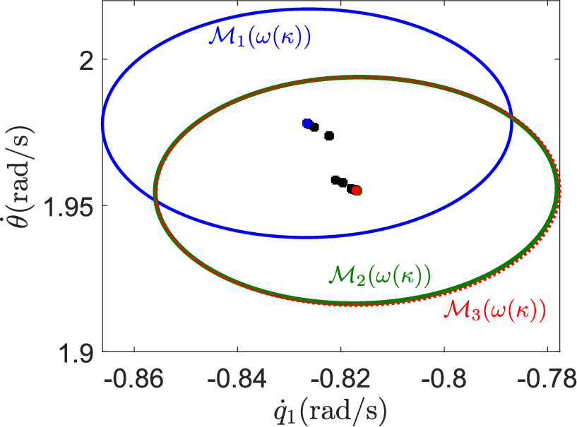
To compute approximate reduced-order planning actions (38) from the actions computed above, we first apply Theorem 1 on the corresponding reduced-order switching system (39). To do this, we follow the procedure outlined in Appendix B-C with the translated reduced-order dynamics , where and . Applying SOS programming, we find that implication (50) in Appendix B-C is satisfied with and , and . Next, selecting and applying (51)-(52) in Appendix B-C we obtain and , resulting in and in the sets , shown in Fig. 5. It is clear that the inclusion (29) is satisfied. Hence, Theorem 1(i) implies that the gait switching system (39) is practically stable with respect to the sets and , which are explicitly computed through the intersection and union of the sets , , respectively. Given the trapping set , we approximate the maps and , by fitting polynomials (41) on an evenly spaced mesh of nodes over the set (40) with ; see Fig. 5. As can be seen from the solid triangles in Fig. 5, the predictions of the approximate displacement maps are almost indistinguishable from the actual ones. More details regarding the polynomial approximations (41) in this example can be found in Appendix D; see also [80] for a video of the resulting motions.
VI Dynamic Walking in Changing Environments
This section describes a primitive-based sequential MPC approach for online planning with limit-cycle walking motions in changing environments. The proposed MPC scheme enables the robot to compute in real time a suitable primitive sequence in the presence of static and moving obstacles; the motion of the latter is assumed to be known. The sequence of primitives suggested by the MPC combines locomotion stability—in the sense of practically stable state evolution of the gait switching system as per Theorem 1—with collision-free paths.
VI-A Practically stable primitive-based predictive planning
We consider a class of reach-avoid navigation problems, wherein a dynamic walker is tasked with reaching a desired (goal) location in an obstacle-cluttered workspace . We will be concerned with both static and moving obstacles. Let denote the static part of ; moving obstacles are not included in . Instead of treating each obstacle in separately, we work with the free space and extract a SWC (SWC) that contains the initial and goal locations and lies entirely in . This allows us to focus on the free space in the vicinity of the robot, decreasing the number of constraints required for collision checking and reducing computation time [81]. The resulting SWC is then used to provide constraints to a sequence of primitive-based MPC programs, which compose the actions in to drive the robot to the goal while keeping its stride-to-stride evolution bounded within the SWC. Finally, moving obstacles are included through additional constraints, thus ensuring reactive composition without re-planning the corridor.
VI-A1 Extracting safe walking corridors
Given and initial and goal locations , a SWC is constructed by computing an ordered collection of pairwise intersecting polytopes in ; the union of these polytopes provides a SWC. Assuming that the obstacles in are convex, this computation can be performed efficiently by the method in [81]. The end result is a sequence of polytopes , , with , , and a collection of waypoints so that
Details can be found in [81]; we only mention here that the method’s computational time scales well with the number of obstacles and that the resulting SWCs capture more free space in than other similar methods.
VI-A2 Safe action composition via sequential MPC
Here, the term “safe” indicates practically stable state evolution of the underlying reduced-order gait switching system (39) combined with collision-free robot displacements. Hitherto, a SWC and a collection of waypoints computed as above are assumed to be given. It is also assumed that a library of reduced-order actions that leads to a practically stable SSME (39) with respect to sets and is available; these actions can be computed as in Section V-C using Theorem 1. To simplify the formulation, we will assume that practical stability is ensured with dwell time constraint . Having this condition is advantageous as it offers the highest degree of flexibility when combining actions, allowing switching to a new gait at each stride without jeopardizing locomotion stability.
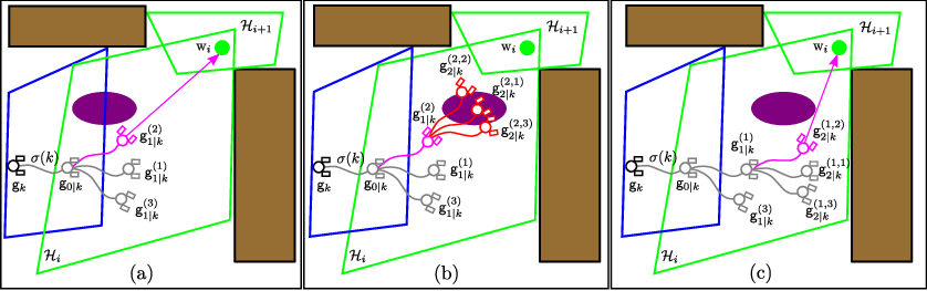
Equipped with a SWC and a library of actions , we now proceed with formulating a corresponding sequence of primitive-based MPC programs that safely drives the robot to the goal. We begin by extracting a collection of approximate reduced-order actions from offline as in Section V-C. The predictive nature of the actions in is then exploited for online planning as follows. Given the robot’s pose , (reduced) state , and primitive index at the beginning of the -th stride, applying the corresponding action provides a prediction of the pose and state of the robot at the beginning of the stride. This prediction is taken as initial condition for the MPC, and is denoted by , and ; see Fig. 6. Subsequent application of actions in results in the corresponding predictions and for the strides that constitute the horizon of the MPC.
With this notation, the objective of MPC is to minimize the distance from the -th waypoint while keeping the predicted robot positions within . To take moving obstacles into account, we assume that the area occupied by the -th moving obstacle can be captured by an ellipse, the position and orientation of which are known over the horizon1212 12 It is assumed that the motion of the moving obstacles is known or can be predicted using a Kalman filter [82]. Only moving obstacles that are within a distance of from the robot’s predicted position are taken into account. Then, for each moving obstacle , the following constraint is incorporated in the MPC programs
To summarize, we have the following sequence of MPC programs that drives the robot to the last polytope :
MPC, :
| {p 0 , …, p N-1 } ∈P minimize | ∑ N ℓ= 1 ∥ w i - p ℓ—k ∥ 2 | (42a) | ||||||||||
| g_k + ~ H _σ(k)—_S ∩Z(z_k) | (42b) | |||||||||||
| ~ P _σ(k)—_S ∩Z(z_k) | (42c) | |||||||||||
| g_ℓ—k + ~ H _p_ℓ—_S ∩Z(z_ℓ—k) | (42d) | |||||||||||
| ~ P _p_ℓ—_S ∩Z(z_ℓ—k) | (42e) | |||||||||||
| H_i⋃H_i+1 | (42f) | |||||||||||
| 1, ν=1,…,n_d | (42g) | |||||||||||
where we note that the constraint (42f) was added in place of the constraint to facilitate transitions between subsequent polytopes when their intersection is small. Once the robot is in , a slightly modified MPC is engaged to drive it to the goal; in MPC, the waypoint in (42a) is replaced with the goal location and the constraint (42f) is replaced by . Owing to the polynomial nature of the approximate actions, the predictions (42d)-(42e) are computed very fast. Solving MPC returns the sequence of indices that minimizes (42a). We then set and proceed with solving MPC at the next stride based on the new initial condition. The process is repeated until for some , where we switch to MPC and continue until the goal.
The MPC programs in (42) rely on the approximate reduced-order planning actions, , rather than the exact ones, . While this choice impacts prediction accuracy to some extent,1313 13 As discussed in [8], its impact is minimal when compared with the predictions by the exact reduced-order actions ; see also Fig. 5. it does not compromise the practical stability properties of the underlying reduced-order switching system (39). This is because the approximate maps derived in (41) and used in (42) to make the requisite predictions do not excite dynamics outside . Hence, if as we assume in this section, the MPC programs (42) have the flexibility to decide to switch to a new primitive at every stride, while the evolution of the system (39) remains practically stable with respect to the sets and associated with the exact action library . If, on the other hand, or an average dwell time constraint is needed, the formulation of the MPC (42) should be modified to incorporate the corresponding constraint. We will refrain from delving deeper into this matter here as it would introduce additional complexity without it being necessary for the examples considered.
Finally, due to the discrete nature of the actions, solving each MPC corresponds to a tree search problem. In (42), at each stage of the MPC all nodes of the tree are expanded using the available primitives; when all nodes are feasible, this expansion results in exponential time complexity , where is the number of gait primitives. To avoid the rapidly increasing computational cost, we will instead employ a modified best first search algorithm to construct the tree online and solve for obstacle-free primitive sequences. The algorithm begins with expanding the primitive tree from using the available actions , as shown in Fig. 6. The expanded nodes that lead to collisions are pruned, and out of the remaining (feasible) ones, the best node—that is, the one closest to the waypoint of MPC (or to the goal for MPC)—is selected for further expansion of the tree. This way only one node is expanded at each stage, resulting in linear time complexity (if all nodes are feasible) at the cost of finding a suboptimal primitive sequence. Note that if at some expansion stage, all nodes lead to collisions, the algorithm backtracks to the previous stage, prunes the best node and selects the second best for expansion. The process is repeated until the algorithm finds a feasible primitive sequence, from which the first one is executed.


VI-B Performance Evaluation
We evaluate the performance of the proposed MPC scheme in simulations with the 3D bipedal robot model of Section V. The dynamics of the robot was integrated in MATLAB using with event detection to detect swing leg touchdown for domain switching. All simulations were performed on an Intel PC with processor ( GHz) and RAM.
VI-B1 Algorithm performance
To assess the efficacy of the primitive-based sequential MPC algorithm described above, we provide numerical evidence on run times and success rates over a large number of randomly generated, highly cluttered environments. We generate these environment by randomly placing rectangular obstacles of varying size and orientation as well as general polytopic obstacles in a confined space keeping the position of the initial and goal point fixed. We consider the cases of 30, 40, 50, and 60 obstacles with the occupancy ratio kept at approximately 40%; see Fig. 7 for an example environment with polytopic obstacles. This way, a total of 600 environments are constructed by generating 150 environments for each obstacle population. For each environment, we use our previous work [81] to generate the SWC connecting the starting and goal locations, which are kept the same across all the environments.
The sequential primitive-based MPC algorithm is then applied to generate collision-free primitive sequences for each environment. The algorithm runs until the robot is within a disc of radius around the goal. To evaluate the effect of the number of primitives used on the success rates and computational time of the algorithm, we consider gait libraries with , , and primitives; these correspond to straight walking ( change in orientation) and turning gaits with nominal orientation changes for the primitives, for the and for the primitives. All primitives are computed as in Section V-C so that practically stable switching with respect to sets and is guaranteed with dwell time bound ; the sets and are similar to those in Fig. 5.
Our results over the 600 environments are summarized in Fig. 7. It can be seen from Fig. 7 that for the same number of primitives, the computational time grows almost linearly with the horizon of the MPC. A similar observation can be made when the horizon is kept constant and the number of primitives increases. This is consistent with the linear lower bound on the complexity of the best first search, indicating that the algorithm did not have to resort to frequent backtracking. Note that in all cases, the MPC run times remain below , which reflects the benefit of using discrete search over a finite library of primitives computed offline. Finally, Fig. 7 shows the corresponding success rates, which, for horizons larger than , exceed .

VI-B2 Moving obstacle avoidance
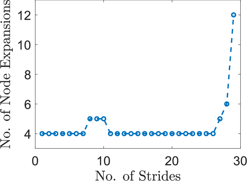
This example illustrates how moving obstacles are treated by the sequential MPC. In what follows, we set the MPC horizon at and use a gait library composed of primitives, which are the same as the ones computed in Section V-C. Figure 8 depicts a workspace with static obstacles, along with a SWC of sequentially overlapping polytopes and the corresponding waypoints. A circular obstacle of radius is moving in the free space along a straight line with a constant speed and its motion is assumed to be known. As shown in Fig. 8, the robot (represented as a red circle) is able to avoid the moving obstacle while staying within the SWC, owing to the added constraint (42g). Note that high-level online planning is combined with practically-stable low-level evolution of the gait switching system (39), as predicted by Theorem 1 and indicated by Fig. 9.
Finally, it is of interest to discuss here how the number of node expansions required by the MPC is affected by the moving obstacle and by the proximity of the goal point to the boundary of the polytope that contains it. Note first that the MPC is solved once per stride. As shown in Fig. 9, when the moving obstacle is far from the robot, the total number of node expansions is , which is equal to the horizon . This indicates that only one node is expanded per stage of the MPC, as expected by the best first search algorithm. However, when the obstacle is in the vicinity of the robot, we observe a slight increase in the number of node expansions, implying that the algorithm utilizes backtracking to suggest a suitable primitive. It can also be seen in Fig. 9 that the node expansion increases abruptly when the robot approaches the goal point. This is because when the robot approaches the goal, the nodes in the primitive tree that are closest to the goal extend outside the polytope, particularly if the goal is close to the polytope boundary. As a result, these nodes are pruned and the algorithm backtracks more frequently to compute a viable primitive sequence. This shortcoming is related to the design of the gait library, which, in this example, uses just three walking gaits with similar stride lengths. This issue can be alleviated easily by enriching the library to include gaits with smaller stride lengths for a more refined reachability tree.
VII Conclusion
This paper presented a rigorous approach towards stable gait composition for reactive planning with dynamic (limit-cycle) walking motions amidst static and moving obstacles. Our approach relies on extracting a library of DMPs in the form of stride maps and their fixed points. These DMPs capture the local dynamics of walking around exponentially stable limit-cycle gaits at the stride level, and the corresponding displacements provide actions available for planning. We identified a general class of 3D bipedal models that enable the decomposition of the problem to high-level planning and low-level gait generation modules. To capture stability aspects, we formulated gait composition as a SSME, and we offered provable stability guarantees under explicit constraints on the frequency of switching. Finally, we proposed a primitive-based sequential MPC to safely drive the robot to the goal while bounding its stride evolution within a SWC and reacting to moving obstacles. The end result is a method that combines collision-free navigation with practically stable locomotion guarantees.
The paper also addressed various implementation aspects towards reducing the computational cost of the method. At the core of our approach lies the idea of dimensional reduction through the enforcement of suitably designed (virtual) holonomic constraints using feedback. This allows the restriction of the planning system on lower-dimensional surfaces and drastically simplifies computations. However, this reduction comes at the cost of guaranteeing stability for the emerging reduced-order planning system. Extending these guarantees to the full-order system requires careful consideration of the effect of unexpected disturbances, model mismatch, and noisy measurements, which violate the assumptions associated with the reduction and will be present in experimental implementations of the method. Addressing these challenges is at the focus of our current work, which examines practical stability in the context of perturbed switched systems; a preliminary result in that direction can be found in [83, Section 6.1.4]. Finally, it is worth mentioning that the tools developed in this paper are relevant to other robots which—like legged robots—move through their environment via periodic interactions.
Appendix A Proof of Propositions 1 and 2
The properties listed in Propositions 1 and 2 are consequences of the symmetries discovered in [69] with the modification of including the position of the robot in .
A-A Proof of Proposition 1
For part (i), it was observed in [69] that the kinetic energy is invariant under the group of rotations of the inertia frame, and thus invariant under yaw rotations ; i.e., rotations about the -axis. Combining this with the observation that yaw rotations also leave the potential energy invariant—for, the -axis of is aligned with gravity—leads to the conclusion that the Lagrangian in (7) is invariant under yaw rotations . Since does not depend on and , we arrive at the conclusion that the vector field in (11) and the corresponding zero-input solutions are equivariant under the action (13), as required.
Part (ii) is a consequence of the flat ground assumption, which implies that the vertical distance of the tip of the swing leg from the ground, which defines by (8), does not depend on translations along the -axes and rotations about the -axis of the inertia frame.
Finally, for part (iii), note that
where is the position at the end of the step of the stance foot (where the body frame is attached) which is the same as its position at the beginning of the step, and is the model’s angular configuration at the end of the step; is a map that provides the coordinates of the swing foot. Next, we show that is equivariant under the action . First, note that based on observations in [69, Section IV-B], the forward kinematics map that associates to each configuration the position and orientation of the tip of the swing foot is equivariant with respect to . Since the map that participates in the first two components of is the part of the forward kinematics map, we deduce that these components are equivariant under yaw rotations. Now, being the identity map, is trivially equivariant with respect to yaw rotations. Finally, by [69, Lemma] the map is also equivariant with respect to , and thus equivariant under yaw rotations. Thus, is equivariant under yaw rotations. Combining this with the fact that only the first two components of depend on and are equivariant under translations along the -axes concludes the proof.
A-B Proof of Proposition 2
Proposition 2 is a direct consequence of Proposition 1 and property (15). To show that is equivariant under the action defined by (13), we will show that its components and are equivariant under . Indeed, if this holds
where the second and third equations follow from the equivariance of and , respectively. Let us focus on showing equivariance of , defined by
where
is the time-to-impact map and . The arguments for the equivariance of are entirely analogous. Note first that by the proof of Proposition 1, and are invariant and is equivariant under . Furthermore, by property (15) the closed-loop flow is equivariant under . Thus, we only need to show that the time-to-impact map is well defined and equivariant under . This effectively follows by the fact that is independent of the coordinates and yaw angle, , since the height of the swing foot that determines the end of the swing phase is independent of these quantities; i.e.,
The proof that is well defined follows from the implicit function theorem applied on .
Appendix B Theorem 1: Discussion, Proof and Application
B-A Discussion: Practical stability and Theorem 1
The notion of practical stability was introduced by LaSalle and Lefschetz in [9, p. 121]. Practical stability neither implies nor is implied by Lyapunov stability; the two concepts are distinct. While the latter provides a qualitative characterization of system behavior, practical stability aims at capturing quantitative aspects of it, such as estimates of solution bounds. Practical stability is essentially a uniform boundedness property of solutions relative to the set . However, it is not merely that a bound exists; the bound is explicitly specified by the set that ensures safe operation. To explain the meaning of these bounds, notice that the ratios in (30) and (32) effectively capture two competing behaviors in the switching system. One is the expansive behavior related to the “jumps” caused by switching, and is captured by the parameter ; the other, is the compressive behavior associated with the exponential decay between switchings, and is captured by the rate . Focusing first on the effect of , note that by (28) a large implies that large “spikes” are possible on switching between subsystems. On the other hand, by (30) and (32), a large also increases the values of and , which, by Definition 3, leads to slower switching. Thus, longer intervals between switchings are enforced, allowing the compressing effect of exponential decay to dominate and keep the state bounded. Similarly when is close to one; i.e., when convergence between switchings is slow.
B-B Proof of Theorem 1
For convenience, the dependence of in (25) and in (27) on will be dropped. Without loss of generality, assume that the system starts at and let . By the definition of , this implies that for all so that no matter what the index of the active system at is. Thus,
| (43) |
Combining (20) with (43), we have
| (44) |
Next, to treat switching, we address parts (i) and (ii) separately.
B-B1 Proof of Theorem 1(i)
Consider any arbitrary (but fixed) switching signal with switching times satisfying Definition 3(i) with (fixed) dwell time constraint (30). Recall that and so (44) implies over . Since by the definition of , we have
| (45) |
As a result, and we distinguish the following cases:
Case (a): .
This case implies that for all so that no matter what the index is. Thus, , and arguing as we did to get (45) we have for all .
Case (b): .
We show that this case is not possible due to the dwell time constraint (30) with1414
14
The dwell-time bound (30) is designed so that Case (b) does not occur. To see this, the arguments in the proof imply that if were true, then for any that is switched in at . But then, due to the fact that , if is large enough so that , we have that for any , which implies that contradicting the original assumption. By Definition 3(i), a switching signal with dwell time satisfies for every pair of switching instants, which, since , implies . This fact, combined with , imply that a switching signal with dwell time that satisfies also satisfies , thus leading to the desired contradiction. The dwell time bound (30) then results from by taking logarithms. . By (26), and thus the fact that implies that . Then, (28) can be used to obtain for all , which by (44) results in for all . Then, since by the definition of the fixed dwell time constraint, we obtain
| (46) |
In view of (30), we have , and so (43) and (46) result in for all . This implies that for any that is “switched in” at , . Thus, , which contradicts our assumption that , essentially guaranteeing that Case (b) does not occur.
B-B2 Proof of Theorem 1(ii)
Our argument for the average dwell time differs from the proof of part (i). This is because we can no longer ensure that every successive switching times are separated by at least a fixed number of steps. Consider again any arbitrary (but fixed) switching signal with switching times satisfying Definition 3(ii) with average dwell time constraint (32). Let be the index of the first switching time for which (28) cannot be applied to bound the value at of the Lyapunov function of the system that is “switched in.” Then, the following claim is true
The proof of this claim is postponed until the end of the main argument, which considers the following cases:
Case (a): .
In this case, the claim applies for all and using (43) we have that for all .
Case (b):
The claim holds over the interval . By the definition of we have that by (26) and the definition of . Hence,
| (47) |
Since and , (47) also implies , and thus we can extend the claim above over the closed interval to get for all . To complete the proof, treat as a new initial time and define . Since (47) corresponds to (43) for the translated time axis, we can re-use the claim exactly as we did above but for the translated time axis to either show for all or to show that the claim can be extended over . These arguments can be propagated indefinitely to show that the solution never leaves , thus concluding the proof.
Proof of the claim: We first show the claim for . By (44) we have for all . Noting that over , we can write for all . Since , and , this inequality implies over . Thus,
| (48) |
which confirms the claim for .
If, on the other hand, so that we can apply (28) to get for all . Thus, no matter what the index is, we arrive at . Noting that for and using (20) we have
This argument can be propagated forward in time as follows. Let be the number of switches over ; note that when , we have . Then, arguing as above we get
By the definition (22) of the average dwell time we have , and substituting we get
for all . Now, recall that and notice that the average dwell time constraint (32) requires with so that . As a result, we obtain the following bound
Note that this bound holds for all and for any ; i.e., it holds for all . Combining this with (48) completes the proof of the claim.
B-C Application of Theorem 1: Relevant Computations
B-C1 Estimation of the BoA
It is beneficial to work with quadratic Lyapunov functions computed via linearization and certified via SOS programming. For convenience, we define the coordinates , with respect to which we have
| (49) |
where and . Since is a locally exponentially stable fixed point for , so is for , and thus the eigenvalues of the linearization are all within the unit disc centered at the origin. Then, a Lyapunov function for (49) over a neighborhood of the origin can be computed by
where is the unique positive definite solution of the discrete Lyapunov equation with positive definite; here, , the identity matrix, for all .
To compute an inner approximation of the BOA of the fixed point of (49), we employ SOS programming. As in [52], we first approximate by its Taylor series up to second order, denoted by . Then, a compact inner approximation of the BOA can be computed by finding the largest for which the implication
| (50) |
can be verified. This is done by formulating the problem as a sequence of SOS feasibility programs [52], which result in the maximum value of .
B-C2 Feasibility and dwell-time constraints
Feasibility of switching among fixed points requires the verification of condition (24), which can be done simply by checking
To apply Theorem 1, a suitable value for the parameter must be determined. This involves the computation of and , which, owing to the quadratic form of the Lyapunov functions can be done in closed form, utilizing the following bounds [10, Proposition 1]
| (51) | ||||
| (52) |
where and and denote the minimum and maximum eigenvalues of the corresponding matrices, respectively.
With these bounds Theorem 1 is applied as follows. For the (fixed) dwell time case, pick a , compute the bound on and check if (29) is satisfied. If it is, compute using the bound on and (30). For the average dwell time, again start with selecting a and compute the bounds on and as above. If the inclusion (31) holds for some , then provide the planner with the numbers where is obtained by (32). In both cases, if the set inclusions (29) or (31) cannot be verified, choose a new and repeat the procedure. Finally, note that for higher-dimensional spaces, checking (29) or (31) can be done using convex optimization tools as in [84, Section 8.4].
B-D Discussion: On fixed versus average dwell time


In general, insisting that the system can switch to a new primitive only after a fixed number of strides are completed may be overly restrictive when in (30). Particularly for path planning in tight environments, a (fixed) dwell time constraint can result in longer paths or even in failure of the planning algorithm to compute a feasible plan. Indeed, let us compare two classes of switching signals, one with a fixed dwell time constraint denoted by and another with an average dwell time constraint with and denoted by ; note that . For the comparison, we use the RRT (RRT) algorithm from [7] with the library of primitives computed in Section V-C over the randomly generated environments of Section VI-A. The algorithm terminates if a path is found that brings the robot within a disc of radius around the goal, or if the number of iterations exceeds 10000. Figure 10 summarizes the results. It can be seen in Fig. 10 that the average dwell time constraint results in higher success rates compared to the fixed dwell time one. Furthermore, Fig. 10 shows that former also results in shorted paths, requiring a smaller number of strides on average. These results provide an indication of the potentially enhanced flexibility offered by the average over the fixed dwell time constraint when .
Appendix C Virtual Constraint Design
In each single support phase, the output (33) has the form
| (53) |
where are the actuated variables and is a monotonic quantity chosen as in [79] to be the angle of the line connecting the point of contact of the support leg with the corresponding hip joint; i.e., . Note that the outputs (53) depend only on , and , as required by (33). Thus, the corresponding output-zeroing controller (34) depends only on the -part of (10) and the equivariance property (15) holds for the closed-loop solutions.
To specify the outputs (53), we begin with the function , which corresponds to third-degree Bezier polynomials designed to generate straight-line walking motions, as in [79, Section IV]. Following the design of , the correction term is introduced in (53) with the purpose of satisfying condition C.1 of Section V-A. This is done by selecting the functions so that the post-impact error of the “uncorrected” part of the output is smoothly driven to zero by the middle of the step; the details can be found in [79, Section V]. The end result is a straight-line, limit-cycle walking gait with local dynamics represented by the reduced-order gait primitive .
Having designed and , we turn our attention to the term , the purpose of which is to obtain turning gaits that satisfy condition C.2 of Section V-A with being the same surface as in . Let and be the values of at the beginning (post-impact) and the end (pre-impact) of a—right or left—step. First, we require
so that when the term does not affect the terms and designed above to obtain the straight-line walking gait ; thus, corresponds to . Next, we define and impose the conditions
| (54) |
so that vanishes at the beginning of the step (when ) and after 90% of the step is completed (when ). Thus, right after one impact and before the next the surfaces agree with the surface of the straight-line gait. As a result, all ’s have a common intersection with and condition C.2 of Section V-A is satisfied; see also Fig. 4.
Now, we are ready to use these constructions to compute limit cycles that correspond to different values of the parameters , and result in turning walking gaits with different changes in orientation. The challenge here is to ensure that the corresponding fixed points are all in the vicinity of . This facilitates provably safe planning by increasing the overlap among the BOAs of the fixed points, and by reducing the dwell time constraint for practical stability of gait switching (39). A simple way to achieve this is as follows. Given a straight-line gait primitive and the corresponding maps and introduce the term so that the conditions (54) are satisfied. The resulting stride map depends on as
| (55) |
where we kept only the orientation component of the displacement map . Note that and , thus these maps are well defined on the reduced-order switching surface associated with primitive .
Linearizing (55) about results in
| (56) |
where and are suitable Jacobians. To find the value of that corresponds to turning by a desired angle without drastically affecting the state part , we substitute and in (56) and solve for to get , where is the right pseudoinverse of . Then, using the and that correspond to the straight-line gait primitive and with computed as above we simulate the system until it converges to a new fixed point which is in the vicinity of and causes turning approximately by . Repeating this procedure for different desired values of turning angle , we obtain different values of . This way, different turning fixed points can be generated, which lie in the vicinity of the straight-line fixed point .
Appendix D Library of Planning Actions in Section V-C

References
- [1] T. McGeer, “Passive dynamic walking,” Int. J. Robot. Res., vol. 9, no. 2, pp. 62–82, 1990.
- [2] S. Collins, A. Ruina, R. Tedrake, and M. Wisse, “Efficient bipedal robots based on passive-dynamic walkers,” Science, vol. 302, pp. 1082–1085, 2005.
- [3] D. Hobbelen and M. Wisse, “Limit cycle walking,” in Humanoid Robots: Human-like Machines, M. Hackel, Ed. Itech, 2007, pp. 277–294.
- [4] A. Ramezani, S.-J. Chung, and S. Hutchinson, “A biomimetic robotic platform to study flight specializations of bats,” Science Robotics, vol. 2, no. 3, 2017.
- [5] C. Georgiades, M. Nahon, and M. Buehler, “Simulation of an underwater hexapod robot,” Ocean Engineering, vol. 36, pp. 39–47, 2009.
- [6] A. J. Ijspeert, J. Nakanishi, H. Hoffmann, P. Pastor, and S. Schaal, “Dynamical movement primitives: Learning attractor models for motor behaviors,” Neural computation, vol. 25, no. 2, pp. 328–373, 2013.
- [7] M. S. Motahar, S. Veer, and I. Poulakakis, “Composing limit cycles for motion planning of 3D bipedal walkers,” in Proc. IEEE Conf. Decis. Control, Las Vegas, December 2016, pp. 6368–6374.
- [8] S. Veer, M. S. Motahar, and I. Poulakakis, “Almost driftless navigation of 3D limit-cycle walking bipeds,” in Proc. IEEE/RSJ Int. Conf. Intell. Robots Syst., 2017, pp. 5025–5030.
- [9] J. LaSalle and S. Lefschetz, Stability by Liapunov’s Direct Method with Applications. Academic Press, New York, 1961.
- [10] S. Veer and I. Poulakakis, “Switched systems with multiple equilibria under disturbances: Boundedness and practical stability,” IEEE Trans. Autom. Control, vol. 65, no. 6, pp. 2371–2386, 2020.
- [11] E. R. Westervelt, J. W. Grizzle, C. Chevallereau, J. H. Choi, and B. Morris, Feedback Control of Dynamic Bipedal Robot Locomotion. Boca Raton, FL: CRC Press, 2007.
- [12] M. A. Sharbafi and A. Seyfarth, Eds., Bioinspired Legged Locomotion. Butterworth-Heinemann, 2017.
- [13] I. Poulakakis and J. W. Grizzle, “Modeling and control of the monopedal robot Thumper,” in Proc. IEEE Int. Conf. Robot. Autom., 2009, pp. 3327–3334.
- [14] A. Ames, K. Galloway, J. Grizzle, and K. Sreenath, “Rapidly exponentially stabilizing control lyapunov functions and hybrid zero dynamics,” IEEE Trans. Autom. Control, vol. 59, no. 4, pp. 876–891, 2014.
- [15] K. A. Hamed and J. W. Grizzle, “Event-based stabilization of periodic orbits for underactuated 3-D bipedal robots with left-right symmetry,” IEEE Trans. Robot., vol. 30, no. 2, pp. 365–381, 2014.
- [16] H. Sadeghian, C. Ott, G. Garofalo, and G. Cheng, “Passivity-based control of underactuated biped robots within hybrid zero dynamics approach,” in Proc. IEEE Int. Conf. Robot. Autom., 2017, pp. 4096–4101.
- [17] G. A. Castillo, B. Weng, W. Zhang, and A. Hereid, “Hybrid zero dynamics inspired feedback control policy design for 3D bipedal locomotion using reinforcement learning,” in Proc. IEEE Int. Conf. Robot. Autom., 2020, pp. 8746–8752.
- [18] A. D. Ames and I. Poulakakis, “Hybrid zero dynamics control of legged robots,” in Bioinspired Legged Locomotion: Models, Concepts, Control and Applications, M. A. Sharbafi and A. Seyfarth, Eds. Butterworth-Heinemann, 2017, pp. 292–331.
- [19] I. R. Manchester and J. Umenberger, “Real-time planning with primitives for dynamic walking over uneven terrain,” in Proc. IEEE Int. Conf. Robot. Autom., 2014, pp. 4639–4646.
- [20] Q. Nguyen and K. Sreenath, “Safety-critical control for dynamical bipedal walking with precise footstep placement,” IFAC-PapersOnLine, vol. 48, no. 27, pp. 147–154, 2015.
- [21] Q. Nguyen, X. Da, J. W. Grizzle, and K. Sreenath, “Dynamic walking on stepping stones with gait library and control barrier functions,” in Algorithmic Foundations of Robotics XII, K. Goldberg, P. Abbeel, K. Bekris, and L. Miller, Eds. Springer, 2020, pp. 384–399.
- [22] R. D. Gregg, T. Bretl, and M. Spong, “Asymptotically stable gait primitives for planning dynamic bipedal locomotion in three dimensions,” in Proc. IEEE Int. Conf. Robot. Autom., 2010, pp. 1695–1702.
- [23] R. D. Gregg, A. K. Tilton, S. Candido, T. Bretl, and M. W. Spong, “Control and planning of 3-D dynamic walking with asymptotically stable gait primitives,” IEEE Trans. Robot., vol. 28, no. 6, pp. 1415–1423, 2012.
- [24] C. Hubicki, M. Jones, M. Daley, and J. Hurst, “Do limit cycles matter in the long run? stable orbits and sliding-mass dynamics emerge in task-optimal locomotion,” in Proc. IEEE Int. Conf. Robot. Autom., 2015, pp. 5113–5120.
- [25] J. P. Hespanha and A. S. Morse, “Stability of switched systems with average dwell-time,” in Proc. IEEE Conf. Decis. Control, 1999, pp. 2655–2660.
- [26] D. Liberzon, Switching in Systems and Control. Boston, MA: Birkhäuser, 2003.
- [27] T. Alpcan and T. Basar, “A stability result for switched systems with multiple equilibria,” J. Dyn. Continuous, Discrete Impulsive Syst. Ser A, Math. Anal., vol. 17, pp. 949–958, 2010.
- [28] X. Da, R. Hartley, and J. W. Grizzle, “First steps toward supervised learning for underactuated bipedal robot locomotion, with outdoor experiments on the wave field,” in Proc. of IEEE Int. Conf. on Robotics and Automation, 2017, pp. 3476–3483.
- [29] Y. Gong, R. Hartley, X. Da, A. Hereid, O. Harib, J.-K. Huang, and J. Grizzle, “Feedback control of a cassie bipedal robot: Walking, standing, and riding a segway,” in Proc. Amer. Control Conf., 2019, pp. 4559–4566.
- [30] Q. Nguyen, A. Agrawal, W. Martin, H. Geyer, and K. Sreenath, “Dynamic bipedal locomotion over stochastic discrete terrain,” Int. J. Robot. Res., vol. 37, no. 13-14, pp. 1537 – 1553, 2018.
- [31] Z. Li, J. Zeng, S. Chen, and K. Sreenath, “Vision-aided autonomous navigation of underactuated bipedal robots in height-constrained environments,” arXiv:2109.05714, 2021.
- [32] C. O. Saglam and K. Byl, “Robust policies via meshing for metastable rough terrain walking,” in Proc. Robot. Sci. Syst., 2014.
- [33] H.-W. Park, A. Ramezani, and J. W. Grizzle, “A finite-state machine for accommodating unexpected large ground-height variations in bipedal robot walking,” IEEE Trans. Robot., vol. 29, no. 2, pp. 331–345, 2013.
- [34] S. Apostolopoulos, M. Leibold, and M. Buss, “Online motion planning over uneven terrain with walking primitives and regression,” in Proc. IEEE Int. Conf. Robot. Autom., 2016, pp. 3799–3805.
- [35] S. Veer, M. S. Motahar, and I. Poulakakis, “Adaptation of limit-cycle walkers for collaborative tasks: A supervisory switching control approach,” in Proc. IEEE/RSJ Int. Conf. Intell. Robots Syst., 2017, pp. 5840–5845.
- [36] S. Veer and I. Poulakakis, “Safe adaptive switching among dynamical movement primitives: Application to 3D limit-cycle walkers,” in Proc. IEEE Int. Conf. Robot. Autom., 2019, pp. 3719–3725.
- [37] P. Chand, S. Veer, and I. Poulakakis, “Interactive dynamic walking: Learning gait switching policies with generalization guarantees,” IEEE Robot. Automat. Lett., vol. 7, no. 2, pp. 4149–4156, 2022.
- [38] ——, “An adaptive supervisory control approach to dynamic locomotion under parametric uncertainty,” in Proc. IEEE Int. Conf. Robot. Autom., 2020, pp. 2443–2449.
- [39] P. A. Bhounsule, A. Zamani, and J. Pusey, “Switching between limit cycles in a model of running using exponentially stabilizing discrete control Lyapunov function,” in Proc. Amer. Control Conf., 2018, pp. 3714–3719.
- [40] A. Zamani, J. D. Galloway, and P. A. Bhounsule, “Feedback motion planning of legged robots by composing orbital lyapunov functions using rapidly-exploring random trees,” in Proc. IEEE Int. Conf. Robot. Autom., 2019, pp. 1410–1416.
- [41] Q. Cao, A. T. van Rijn, and I. Poulakakis, “On the control of gait transitions in quadrupedal running,” in Proc. IEEE/RSJ Int. Conf. Intell. Robots Syst., Sep. 2015, pp. 5136 – 5141.
- [42] Q. Cao and I. Poulakakis, “Quadrupedal running with a flexible torso: Control and speed transitions with sums-of-squares verification,” Artificial Life and Robotics, vol. 21, no. 4, pp. 384–392, 2016.
- [43] W. Ubellacker, N. Csomay-Shanklin, T. G. Molnar, and A. D. Ames, “Verifying safe transitions between dynamic motion primitives on legged robots,” in Proc. IEEE/RSJ Int. Conf. Intell. Robots Syst., 2021, pp. 8477–8484.
- [44] S. Veer and I. Poulakakis, “Practical stability of switched systems with multiple equilibria under disturbances,” in Proc. Amer. Control Conf., 2019.
- [45] M. Dorothy and S.-J. Chung, “Switched systems with multiple invariant sets,” Syst. Control Lett., vol. 96, pp. 103–109, 2016.
- [46] W. M. Haddad and V. Chellaboina, Nonlinear Dynamical Systems and Control: A Lyapunov-Based Approach. Princeton, NJ: Princeton University Press, 2008.
- [47] R. R. Burridge, A. A. Rizzi, and D. E. Koditschek, “Sequential composition of dynamically dexterous robot behaviors,” Int. J. Robot. Res., vol. 18, no. 6, pp. 534–555, 1999.
- [48] M. Mason, “The mechanics of manipulation,” in Proc. IEEE Int. Conf. Robot. Autom., 1985, pp. 544–548.
- [49] T. Lozano-Pèrez, M. T. Mason, and R. H. Taylor, “Automatic synthesis of fine-motion strategies for robots,” Int. J. Robot. Res., vol. 3, no. 1, pp. 3–23, 1984.
- [50] P. A. Parrilo, “Structured semidefinite programs and semialgebraic geometry methods in robustness and optimization,” Ph.D. dissertation, California Institute of Technology, 2000.
- [51] S. M. LaValle and J. J. Kuffner, “Randomized kinodynamic planning,” Int. J. Robot. Res., vol. 20, no. 5, pp. 378–400, 2001.
- [52] R. Tedrake, I. R. Manchester, M. Tobenkin, and J. W. Roberts, “LQR-trees: Feedback motion planning via sums-of-squares verification,” Int. J. Robot. Res., vol. 29, no. 8, pp. 1038–1052, 2010.
- [53] A. Majumdar and R. Tedrake, “Funnel libraries for real-time robust feedback motion planning,” Int. J. Robot. Res., vol. 36, no. 8, pp. 947–982, 2017.
- [54] C. Danielson, A. Weiss, K. Berntorp, and S. Di Cairano, “Path planning using positive invariant sets,” in Proc. IEEE Conf. Decis. Control, 2016.
- [55] A. Weiss, C. Danielson, K. Berntorp, I. Kolmanovsky, and S. Di Cairano, “Motion planning with invariant set trees,” in Proc. Conf. Control Technol. Appl., 2017, pp. 1625–1630.
- [56] F. S. Barbosa, L. Lindemann, D. V. Dimarogonas, and J. Tumova, “Provably safe control of Lagrangian systems in obstacle-scattered environments,” in Proc. IEEE Conf. Decis. Control, 2020, pp. 2056–2061.
- [57] S. Li, D. Park, Y. Sung, J. A. Shah, and N. Roy, “Reactive task and motion planning under temporal logic specifications,” in Proc. IEEE Int. Conf. Robot. Autom., 2021, pp. 12 618–12 624.
- [58] V. Vasilopoulos, S. Castro, W. Vega-Brown, D. E. Koditschck, and N. Roy, “A hierarchical deliberative-reactive system architecture for task and motion planning in partially known environments,” in Proc. IEEE Int. Conf. Robot. Autom., 2022, pp. 7342–7348.
- [59] A. Shamsah, Z. Gu, J. Warnke, S. Hutchinson, and Y. Zhao, “Integrated task and motion planning for safe legged navigation in partially observable environments,” arXiv:2110.12097, 2021.
- [60] P.-B. Wieber, R. Tedrake, and S. Kuindersma, “Modeling and control of legged robots,” in Springer Handbook of Robotics, B. Sicialiano and O. Khatib, Eds. Springer, 2016, pp. 1203–1234.
- [61] P. M. Wensing and S. Revzen, “Template models for control,” in Bioinspired Legged Locomotion: Models, Concepts, Control and Applications, M. A. Sharbafi and A. Seyfarth, Eds. Butterworth-Heinemann, 2017, pp. 240–263.
- [62] S. Kajita, F. Kanehiro, K. Kaneko, K. Yokoi, and H. Hirukawa, “The 3D linear inverted pendulum mode: A simple modeling for a biped walking pattern generation,” in Proc. IEEE/RSJ Int. Conf. Intell. Robots Syst., 2001, pp. 239–246.
- [63] I. Poulakakis and J. W. Grizzle, “The spring loaded inverted pendulum as the hybrid zero dynamics of an asymmetric hopper,” IEEE Trans. Autom. Control, vol. 54, no. 8, pp. 1779–1793, 2009.
- [64] I. Poulakakis, “Spring loaded inverted pendulum embedding: Extensions toward the control of compliant running robots,” in Proc. IEEE Int. Conf. Robot. Autom., 2010, pp. 5219–5224.
- [65] V. Kurtz, P. M. Wensing, and H. Lin, “Approximate simulation for template-based whole-body control,” IEEE Robot. Automat. Lett., vol. 6, no. 2, pp. 558–565, 2021.
- [66] S. Veer, Rakesh, and I. Poulakakis, “Input-to-state stability of periodic orbits of systems with impulse effects via Poincaré analysis,” IEEE Trans. Autom. Control, vol. 64, no. 11, pp. 4583–4598, 2019.
- [67] S. Veer and I. Poulakakis, “Robustness of periodic orbits of impulsive systems à la Poincaré,” in Proc. IEEE Int. Conf. on Dec. Control, 2019, pp. 3966–3971.
- [68] A. Isidori, Nonlinear Control Systems, 3rd ed. New York: Springer, 1995.
- [69] M. W. Spong and F. Bullo, “Controlled symmetries and passive walking,” IEEE Trans. Autom. Control, vol. 50, no. 7, pp. 1025–1031, 2005.
- [70] C.-L. Shih, J. Grizzle, and C. Chevallereau, “From stable walking to steering of a 3D bipedal robot with passive point feet,” Robotica, vol. 30, no. 07, pp. 1119–1130, 2012.
- [71] G. Zhai and A. N. Michel, “Generalized practical stability analysis of discontinuous dynamical systems,” in Proc. IEEE Conf. Decis. Control, 2003, pp. 1663–1668.
- [72] A. Majumdar and R. Tedrake, “Robust online motion planning with regions of finite time invariance,” in Algorithmic Foundations of Robotics X, E. Frazzoli, T. Lozano-Perez, N. Roy, and D. Rus, Eds. Springer, 2013, pp. 543–558.
- [73] C. Chevallereau, J. Grizzle, and C.-L. Shih, “Steering of a 3D bipedal robot with an underactuated ankle,” in Proc. IEEE/RSJ Int. Conf. Intell. Robots Syst., 2010.
- [74] R. D. Gregg and M. W. Spong, “Reduction-based control of three-dimensional bipedal walking robots,” Int. J. Robot. Res., vol. 29, no. 6, pp. 680–702, 2009.
- [75] R. W. Sinnet and A. D. Ames, “3D bipedal walking with knees and feet: A hybrid geometric approach,” in Proc. IEEE Conf. Decis. Control, Shanghai, P.R. China, December 2009, pp. 3208–3213.
- [76] M. W. Spong, J. K. Holm, and D. Lee, “Passivity- based control of bipedal locomotion,” IEEE Robot. Automat. Mag., vol. 12, no. 2, pp. 30–40, 2007.
- [77] Q. Nguyen and K. Sreenath, “Optimal robust control for bipedal robots through control lyapunov function based quadratic programs,” in Proc. Robot. Sci. Syst., 2015.
- [78] J. W. Grizzle, C. Chevallereau, R. W. Sinnet, and A. D. Ames, “Models, feedback control, and open problems of 3d bipedal robotic walking,” Automatica, vol. 50, no. 8, pp. 1955–1988, 2014.
- [79] C. Chevallereau, J. W. Grizzle, and C.-L. Shih, “Asymptotically stable walking of a five-link underactuated 3-D bipedal robot,” IEEE Trans. Robot., vol. 25, no. 1, pp. 37–50, 2009.
- [80] Simulation results. [Online]. Available: https://youtu.be/FYRBuWOqKww
- [81] K. S. Narkhede, A. M. Kulkarni, D. A. Thanki, and I. Poulakakis, “A sequential MPC approach to reactive planning for bipedal robots using safe corridors in highly cluttered environments,” IEEE Robot. Automat. Lett., vol. 7, no. 4, pp. 11 831–11 838, 2022.
- [82] B. Brito, B. Floor, L. Ferranti, and J. Alonso-Mora, “Model predictive contouring control for collision avoidance in unstructured dynamic environments,” IEEE Robot. Automat. Lett., vol. 4, no. 4, pp. 4459–4466, 2019.
- [83] S. Veer, “Composing motion primitives under disturbances: A switched systems approach,” Ph.D. dissertation, University of Delaware, 2018.
- [84] S. Boyd and L. Vandenberghe, Convex Optimization. Cambridge University Press, 2004.