Electron- $K$ -Phonon Interaction In Twisted Bilayer Graphene

Chao-Xing Liu^∗ Affiliation: Department of Physics, The Pennsylvania State University, University Park, Pennsylvania 16802, USA Affiliation: Department of Physics, Princeton University, Princeton, NJ 08544 Yulin Chen Affiliation: Department of Physics, University of Oxford, Oxford, OX1 3PU, United Kingdom Ali Yazdani Affiliation: Department of Physics, Princeton University, Princeton, NJ 08544 B. Andrei Bernevig^∗ Affiliation: Department of Physics, Princeton University, Princeton, NJ 08544 Affiliation: Donostia International Physics Center, P. Manuel de Lardizabal 4, 20018 Donostia-San Sebastian, Spain Affiliation: IKERBASQUE, Basque Foundation for Science, Bilbao, Spain

August 11, 2026

Abstract

We develop an analytic theory to describe the interaction between electrons and $K$ -phonons and study its influence on superconductivity in the bare bands of twisted bilayer graphene (TBG). We find that, due to symmetry and the two-center approximation, only one optical $K$ phonon ( $\sim 160meV$ ) of graphene is responsible for inter-valley electron-phonon interaction. This phonon has recently been found in angular-resolved photo-emission spectroscopy to be responsible for replicas of the TBG flat bands. By projecting the interaction to the TBG flat bands, we perform the full symmetry analysis of phonon-mediated attractive interaction and pairing channels in the Chern basis, and show that several channels are guaranteed to have gapless order parameters. From the linearized gap equations, we find that the highest $T_{c}$ pairing induced by this phonon is a singlet gapped s-wave inter-Chern-band order parameter, followed closely by a gapless nematic d-wave intra-Chern-band order parameter. We justify these results analytically, using the topological heavy fermion mapping of TBG which has allowed us to obtain an analytic form of phonon-mediated attractive interaction and to analytically solve the linearized and $T=0$ gap equations. For the intra-Chern-band channel, the nematic state with nodes is shown to be stabilized in the chiral flat band limit. While the flat band Coulomb interaction can be screened sufficiently enough - around Van-Hove singularities - to allow for electron-phonon based superconductivity, it is unlikely that this effect can be maintained in the lower density of states excitation bands around the correlated insulator states.

pacs

73.43.-f, 71.10.Fd, 03.65.Vf, 03.65.Ud

Introduction - Superconductivity in twisted bilayer graphene (TBG) appears within its phase diagram around the correlated insulator states Cao et al. 2018a; Cao et al. 2018b; Lu et al. 2019; Codecido et al. 2019; Yankowitz et al. 2019; Cao et al. 2021; Oh et al. 2021; Liu et al. 2021; Saito et al. 2020; Arora et al. 2020; Codecido et al. 2019; Andrei and MacDonald 2020; Liu and Dai 2021; Kwan et al. 2021; Nuckolls et al. 2023; Călugăru et al. 2022; Kang et al. 2021; Kang and Vafek 2018; Kang and Vafek 2019; Vafek and Kang 2020. Amongst the mechanisms suggested for superconductivity are the phonons, spin fluctuations, skyrmions, and others Khalaf et al. 2021; Khalaf et al. 2022; Po et al. 2018; You and Vishwanath 2019; Lian et al. 2019; Wu et al. 2018; Wu 2019; Wu et al. 2019; Wu and Sarma 2019; Chichinadze et al. 2020; Fernandes and Fu 2021; Wang et al. 2021; Yu et al. 2022a; Sharma et al. 2020; Isobe et al. 2018; Roy and Juričić 2019; Peltonen et al. 2018; Chichinadze et al. 2020; Kennes et al. 2018; Gonzalez and Stauber 2019; Cea and Guinea 2021; Shavit et al. 2021; Liu et al. 2018; Fidrysiak et al. 2018; Sharma et al. 2020; Chou et al. 2019; Kozii et al. 2019; You and Vishwanath 2019; Wang et al. 2021. Based on a recent experiment that suggest a strong coupling between the graphene $K$ -phonon and the flat bands in TBG che, we perform a comprehensive analysis of the electron- $K$ -phonon (e-K-ph) interaction and the resulting phonon-mediated superconductivity on the bare flat bands of TBG. We develop an exhaustive numerical, analytical, and symmetry based description of the e-K-ph interaction in TBG and the symmetry classifications of the order parameter, and find the competing singlet gapped inter-Chern-band channel and nematic gapless intra-Chern-band channel. Armed with the heavy-fermion description of TBGSong and Bernevig 2022; Călugăru et al. 2023; Hu et al. 2023a; Hu et al. 2023b; Lau and Coleman 2023; Datta et al. 2023; Yu et al. 2023; Chou and Sarma 2022; Zhou and Song 2023, the form factors of the $K$ -phonon induced attractive interaction can be analytically computed and matched well to a full numerical calculations. An analysis of the Coulomb screening shows that, due to the high density of states (DOS) of flat bands, the Coulomb interaction might be strongly renormalized down near the Van Hove singularities. However, it remains unclear if the Hartree-Fock bands of the correlated insulator, with the lower DOS, can provide a similar result.

Model Hamiltonian for electron-phonon interaction in TBG - We consider the deformation potential type of theory, described by a tight-binding (TB) model for the electron Hamiltonian with the hopping parameters depending on the atom positions $\tilde{\bf R}_{\alpha}^{l}={\bf R}^{l}+{\bf\tau}_{\alpha}^{l}+{\bf u}^{l}({\bf R}^{l}_{\alpha})$ with a displacement field ${\bf u}^{l}({\bf R}^{l}_{\alpha}={\bf R}^{l}+{\bf\tau}_{\alpha}^{l})$ , where ${\bf R}^{l}$ and ${\bf\tau}_{\alpha}^{l}$ label the lattice vector and the sublattice atom position ( $\alpha=A,B$ ) at the layer $l$ , respectively. By treating ${\bf u}$ as a perturbation, we expand the intra-layer Hamiltonian up to the linear order in $\mathbf{u}$ (Supplementary Material (SM) Sec. II sm2). We only keep $\mathbf{u}$ -independent terms for the inter-layer Hamiltonian for TBG, thus focusing on intra-layer electron-phonon (e-ph) interaction in this work. As only the Dirac bands appear around the Fermi energy close to $\pm\mathbf{K}_{D}=\pm\frac{4\pi}{3a_{0}}(1,0)$ in Brillouin zone (BZ) with lattice constant $a_{0}$ in graphene, we also expand the Hamiltonian around $\eta\mathbf{K}_{D}$ ( $\eta=\pm$ labelling two valleys) and focus on Dirac electrons around two valleys. Our full Hamiltonian consists of three parts

\displaystyle H=H_{el}+H_{ph}+H_{eph}.

(1)

Here $H_{el}$ describes the Dirac electrons located at valley $\eta=\pm$ momentum $\eta\mathbf{K}_{D}$ that are coupled through inter-layer tunnelings and is given by the Bistritzer-MacDonald (BM) model Bistritzer and MacDonald 2011 (SM Sec. V sm2),

{\hat{H}}_{\rm el}=\sum_{\eta s}\sum_{\mathbf{k}\in{\rm MBZ}}\sum_{\alpha\alpha^{\prime}}\sum_{\mathbf{Q},\mathbf{Q}^{\prime}}h_{\mathbf{Q}\alpha,\mathbf{Q}^{\prime}\alpha^{\prime}}^{(\eta)}(\mathbf{k})c_{\mathbf{k},\mathbf{Q},\alpha,\eta,s}^{\dagger}c_{\mathbf{k},\mathbf{Q}^{\prime},\alpha^{\prime},\eta,s}

(2)

where $c_{\mathbf{k},\mathbf{Q},\alpha,\eta,s}$ is the fermion annihilation operator $\mathbf{k}$ is a momentum in the Moiré Brillouin zone (MBZ) (Fig. 1b), $\alpha$ is the sublattice index, and $s$ is spin. The vector $\mathbf{Q}$ belongs to the lattice set $\mathcal{Q}_{l\eta}=\{l\eta\mathbf{q}_{2}+n_{1}\mathbf{b}_{M1}+n_{2}\mathbf{b}_{M2}\ |\ n_{1,2}\in\mathbb{Z}\}$ , where $l$ is the layer index, $\mathbf{q}_{2}=k_{\theta}(\frac{\sqrt{3}}{2},\frac{1}{2})$ , $\mathbf{b}_{M1}=k_{\theta}(\frac{\sqrt{3}}{2},\frac{3}{2})$ , $\mathbf{b}_{M2}=k_{\theta}(-\frac{\sqrt{3}}{2},\frac{3}{2})$ and $k_{\theta}=2|\mathbf{K}_{D}|\sin\frac{\theta}{2}$ with $\theta$ the twist angle. $h_{\mathbf{Q}\alpha,\mathbf{Q}^{\prime}\alpha^{\prime}}^{(\eta)}(\mathbf{k})$ is given in SM Sec. V.A sm2. ${\hat{H}}_{\rm el}$ exhibits $C_{6v}$ and time-reversal symmetries, generated by valley-switching $\pi/6$ -rotation along z axis ( $\hat{C}_{6z}$ ), time reversal ( $\hat{T}$ ), and $\pi$ -rotation along y axis ( $C_{2y}$ ), and valley-preserving $\pi$ -rotation along x axis ( $\hat{C}_{2x}$ ), and the composite anti-unitary $C_{2z}T$ . In addition, ${\hat{H}}_{\rm el}$ has a unitary particle-hole ( $\hat{P}$ ) symmetry, as well as a chiral symmetry $\hat{C}$ in the limit with vanishing $AA$ region hopping ( $w_{0}=0$ ) Vafek and Kang 2020. A full discussion of symmetry of BM model Bernevig et al. 2021; Song et al. 2021 is found in SM Sec.V.B sm2.

$H_{ph}$ describes the intra-layer in-plane phonon modes. Out-of-plane phonon modes are decoupled from Dirac electrons for intra-layer e-ph interaction. The dynamical matrix for a single layer graphene is derived in SM Sec.III sm2 based both on symmetry considerations and the microscopic model, up to the next nearest neighbor interaction. The resulting in-plane phonon dispersion in Fig. 1a reproduces that in literature Neto et al. 2009; Sahoo and Mishra 2012; Thingstad et al. 2020; Maultzsch et al. 2004; Mohr et al. 2007 (SM Sec.III and IV.B sm2). The phonon modes at $\Gamma$ and $\eta\mathbf{K}_{D}$ can induce intra-valley and inter-valley e-ph interactions, respectively. In this paper we focus on the $\eta\mathbf{K}_{D}$ phonons; the $\Gamma$ phonons will be derived in liu. At $\eta\mathbf{K}_{D}$ , we have one $A_{1}$ ( $\sim 160meV$ ), one $A_{2}$ ( $\sim 140meV$ ) and one 2D $E$ mode ( $\sim 150meV$ ) of $C_{3v}$ group. Based on the deformation potential theory, we derive the e-ph interaction $H_{eph}$ by expanding the TB Hamiltonian treating both the momentum and phonon displacement field $\mathbf{u}$ as perturbations. For e-ph interaction, we only keep the dominant zeroth-order in momentum for the $\eta\mathbf{K}_{D}$ phonons. We find, due to both symmetry and the two-center approximation (SM Sec.II.E sm2), that only the $A_{1}$ phonons at $\mathbf{K}_{D}$ can scatter an electron from $\mathbf{K}_{D}$ to $-\mathbf{K}_{D}$ Mohr et al. 2007. The corresponding Hamiltonian reads

\displaystyle H_{inter-vall}^{op,A_{1}}\approx\frac{\gamma_{3}}{\sqrt{2N_{G}M\omega_{A1}}}\sum_{\tilde{\mathbf{k}},\tilde{\mathbf{k}}^{\prime},\eta,\alpha\beta}(b_{-\eta\mathbf{K}_{D}+\tilde{\mathbf{k}}-\tilde{\mathbf{k}}^{\prime},A_{1}}+b_{\eta\mathbf{K}_{D}-\tilde{\mathbf{k}}+\tilde{\mathbf{k}}^{\prime},A_{1}}^{\dagger})c^{\dagger}_{\tilde{\mathbf{k}}+\eta\mathbf{K}_{D},\alpha}(\sigma_{x})_{\alpha\beta}c_{\tilde{\mathbf{k}}^{\prime}-\eta\mathbf{K}_{D},\beta},

(3)

where $\tilde{\mathbf{k}}$ is the electron momentum away from $\eta\mathbf{K}_{D}$ , $N_{G}$ is the number of atomic unit cells, $M$ is the atomic mass, $\omega_{A1}$ is the $A_{1}$ phonon frequency, and $b$ and $c$ are phonon and electron annihilation operators. The material dependent parameter $\gamma_{3}$ can be derived from the hopping potential as $\gamma_{3}=2i\sum_{\mathbf{G}}e^{i(\tau_{A}-\tau_{B})\cdot\mathbf{G}}(\mathbf{G}+\mathbf{K}_{D})_{y}t(\mathbf{G}+\mathbf{K}_{D},0)\approx 17\text{eV/ \AA}$ , where $\mathbf{G}$ is the reciprocal lattice vector and $t(\mathbf{q})$ is the Fourier transform of the $\pi$ -bond hopping function between two carbon $p_{z}$ orbitals in graphene (Eq. 6 in SM Sec.I sm2). Our next step is to re-write the electron momentum $\tilde{k}$ into the MBZ by $\tilde{\mathbf{k}}=\mathbf{k}-\mathbf{Q}_{l\eta}$ with $\mathbf{k}\in\text{MBZ}$ , so that $c_{\mathbf{k},\mathbf{Q}_{l\eta},\alpha,\eta,s}=c_{\eta\mathbf{K}_{D}^{l}+\tilde{\mathbf{k}},\alpha,l,s}$ and $\sum_{\tilde{\mathbf{k}}}\rightarrow\sum_{\mathbf{k}\in\text{MBZ}}\sum_{\mathbf{Q}_{l\eta}}$ , where we have added the spin index $s$ and layer index $l$ . Finally, we project the e-ph interaction $H_{inter-vall}^{op,A_{1}}$ into the flat bands of the BM Hamiltonian as

	$\displaystyle H_{inter-vall}^{op,A_{1}}\approx\frac{1}{\sqrt{N_{G}}}\sum G_{\mathbf{k},\mathbf{k}^{\prime},\mathbf{Q}_{-l\eta}}^{\eta nn^{\prime}l}\gamma_{\mathbf{k},n,\eta,s}^{\dagger}\gamma_{\mathbf{k}^{\prime},n^{\prime},-\eta,s}$
	$\displaystyle(b_{-\eta\mathbf{K}_{D}+\mathbf{k}-\mathbf{k}^{\prime}-\mathbf{Q}_{-l\eta},l,A_{1}}+b_{\eta\mathbf{K}_{D}-\mathbf{k}+\mathbf{k}^{\prime}+\mathbf{Q}_{-l\eta},l,A_{1}}^{\dagger})$		(4)

where the summation includes $\mathbf{k},\mathbf{k}^{\prime},n,n^{\prime},\eta,s,l,\mathbf{Q}_{-l\eta}$ , $\gamma_{\mathbf{k},n,\eta,s}^{\dagger}=\sum_{\mathbf{Q}\alpha}u_{\mathbf{Q}\alpha;n\eta}\left(\mathbf{k}\right)c_{\mathbf{k},\mathbf{Q},\eta,\alpha s}^{\dagger}$ with $u^{n}_{\mathbf{k},\mathbf{Q}^{\prime}_{l\eta},\alpha,\eta}$ the eigenstates of $h_{\mathbf{Q}\alpha,\mathbf{Q}^{\prime}\alpha^{\prime}}^{(\eta)}(\mathbf{k})$ . The matrix element

	$\displaystyle G_{\mathbf{k},\mathbf{k}^{\prime},\mathbf{Q}_{-l\eta}}^{\eta nn^{\prime}l}=\frac{\gamma_{3}}{\sqrt{2M\omega_{A_{1}}}}\sum_{\mathbf{Q}^{\prime}_{l\eta},\alpha\beta}$
	$\displaystyle u^{n\star}_{\mathbf{k},\mathbf{Q}^{\prime}_{l\eta},\alpha,\eta}\sigma^{x}_{\alpha\beta}u^{n^{\prime}}_{\mathbf{k}^{\prime},\mathbf{Q}^{\prime}_{l\eta}-\mathbf{Q}_{-l\eta},\beta,-\eta}$		(5)

characterizes the e-ph interaction strength for TBG and can be evaluated numerically (and later analytically), as shown in SM Sec. VI.F sm2. We focus on two flat bands (per valley per spin) of TBG, labelled by $n=\pm$ . Instead of the eigen-state basis, we work on the so-called ”Chern-band” basis, defined by

u^{e_{Y}}_{\mathbf{k},\mathbf{Q},\alpha,\eta}=\frac{1}{\sqrt{2}}(u^{n=+}_{\mathbf{k},\mathbf{Q},\alpha,\eta}+ie_{Y}u^{n=-}_{\mathbf{k},\mathbf{Q},\alpha,\eta})

(6)

with $e_{Y}=\pm 1$ . $u^{e_{Y}}_{\mathbf{k},\mathbf{Q},\alpha,\eta}$ carries the Chern number $\pm 1$ . On the Chern-band basis, the expressions for e-ph interaction can be obtained by replacing the $n,n^{\prime}$ indices in Eqs. (Electron- $K$ -Phonon Interaction In Twisted Bilayer Graphene) and (Electron- $K$ -Phonon Interaction In Twisted Bilayer Graphene) with $e_{Y},e^{\prime}_{Y}$ indices and $u^{n}_{\mathbf{k},\mathbf{Q},\alpha,\eta}$ in Eq. (Electron- $K$ -Phonon Interaction In Twisted Bilayer Graphene) with $u^{e_{Y}}_{\mathbf{k},\mathbf{Q},\alpha,\eta}$ . Discrete symmetries can constrain the form of the function $G_{\mathbf{k},\mathbf{k}^{\prime},\mathbf{Q}_{-l\eta}}^{\eta e_{Y}e_{Y}^{\prime}l}$ , as discussed in SM Sec.VI.D sm2. In particular, in the chiral limit $w_{0}=0$ one can show that $G_{\mathbf{k},\mathbf{k}^{\prime},\mathbf{Q}_{-l\eta}}^{\eta e_{Y}e_{Y}^{\prime}l}=\delta_{e_{Y},e_{Y}^{\prime}}G_{\mathbf{k},\mathbf{k}^{\prime},\mathbf{Q}_{-l\eta}}^{\eta e_{Y}e_{Y}l}$ has diagonal form on the Chern-band basis.

Phonon-mediated Electron-electron Interaction and Symmetry Classification of Superconducting Pairing Channels - We next apply the Schrieffer-Wolff transformation Schrieffer and Wolff 1966 to integrate out the phonon modes and obtain the phonon-mediated electron-electron (el-el) interaction Wu et al. 2018; Yu et al. 2022a. We focus on the Cooper pair channel of the attractive interaction, which takes the form

	$\displaystyle H_{ee}=-\frac{1}{N_{M}}\sum_{\mathbf{k},\mathbf{k}^{\prime},s,s_{1},e_{Y},e_{Y}^{\prime}}V^{\eta,e_{Y},e_{Y}^{\prime}}_{\mathbf{k},\mathbf{k}^{\prime}}$
	$\displaystyle\gamma_{\mathbf{k}e_{Y}\eta s}^{\dagger}\gamma_{-\mathbf{k}e^{\prime}_{Y},-\eta s_{1}}^{\dagger}\gamma_{-\mathbf{k}^{\prime}e^{\prime}_{Y},\eta s_{1}}\gamma_{\mathbf{k}^{\prime}e_{Y},-\eta s},$		(7)

where

V^{\eta,e_{Y},e_{Y}^{\prime}}_{\mathbf{k},\mathbf{k}^{\prime}}=\frac{1}{N_{0}\omega_{A_{1}}}\sum_{\mathbf{G}_{M},l}G_{\mathbf{k},\mathbf{k}^{\prime},-l\eta\mathbf{q}_{2}+\mathbf{G}_{M}}^{\eta,e_{Y},l}G_{-\mathbf{k},-\mathbf{k}^{\prime},l\eta\mathbf{q}_{2}-\mathbf{G}_{M}}^{-\eta,e_{Y}^{\prime},l}

with $\mathbf{G}_{M}$ the Moiré reciprocal lattice vectors, $N_{M}$ the number of Moiré unit cells and $N_{0}$ the number of atomic unit cells in one Moiré unit cell ( $N_{G}=N_{0}\times N_{M}$ ). Discrete symmetries constrain the form of the interaction parameter $V^{\eta,e_{Y},e_{Y}^{\prime}}_{\mathbf{k},\mathbf{k}^{\prime}}$ . The ones leaving the momentum $(\mathbf{k},\mathbf{k}^{\prime})$ unchanged are: (1) $\hat{C}_{2z}\hat{P}$ : $V^{\eta,e_{Y},e_{Y}^{\prime}}_{\mathbf{k},\mathbf{k}^{\prime}}=V^{-\eta,e_{Y},e_{Y}^{\prime}}_{\mathbf{k},\mathbf{k}^{\prime}}$ ; (2) $\hat{C}_{2z}\hat{T}$ : $V^{\eta,e_{Y},e_{Y}^{\prime}}_{\mathbf{k},\mathbf{k}^{\prime}}=V^{\eta,-e_{Y},-e_{Y}^{\prime}\star}_{\mathbf{k},\mathbf{k}^{\prime}}$ ; and (3) the combination of index reshuffling and $\hat{P}$ symmetry: $V^{\eta,e_{Y}e_{Y}^{\prime}}_{\mathbf{k},\mathbf{k}^{\prime}}=V^{-\eta,e_{Y}^{\prime}e_{Y}}_{\mathbf{k},\mathbf{k}^{\prime}}$ . These three symmetry operations reduce the number of the independent components of the $V$ -function for a fixed $(\mathbf{k},\mathbf{k}^{\prime})$ from 8 complex parameters to 1 real ( $V^{+,+-}_{\mathbf{k},\mathbf{k}^{\prime}}$ ) and 1 complex parameter ( $V^{+,++}_{\mathbf{k},\mathbf{k}^{\prime}}$ ). Other discrete symmetries, including $\hat{P}$ , reshuffling, hermicity, $\hat{C}_{3z}$ and $\hat{C}_{2z}$ , relate the $V$ -function at different $(\mathbf{k},\mathbf{k}^{\prime})$ . In particular, $\hat{C}_{3z}$ guarantees $V^{\eta,e_{Y},e_{Y}}_{\mathbf{K}_{M},0}=0$ for the intra-Chern-band channels. The projected Coulomb interaction into the flat bands of the BM model possesses a large $U(4)\times U(4)$ spin-valley continuous symmetry Bernevig et al. 2021; Kang and Vafek 2019; Bultinck et al. 2020. the el-el interaction (Electron- $K$ -Phonon Interaction In Twisted Bilayer Graphene) breaks this symmetry down to the $U(2)_{e_{Y}=+}\times U(2)_{e_{Y}=-}$ in the chiral limit and further to a total spin $SU(2)$ together with a valley charge $U(1)\otimes U(1)$ (SM Sec.VI.E sm2).

At the mean field level, the attractive interaction (Electron- $K$ -Phonon Interaction In Twisted Bilayer Graphene) is decomposed into the fermion bilinear form $H_{\Delta}=\hat{\Delta}+\hat{\Delta}^{\dagger}$ with

\hat{\Delta}=\sum\gamma_{\mathbf{k},e_{Y_{1}},\eta,s_{1}}^{\dagger}\Delta^{\eta}_{\mathbf{k};e_{Y_{1}}s_{1},e_{Y_{2}}s_{2}}\gamma_{-\mathbf{k},e_{Y_{2}},-\eta,s_{2}}^{\dagger},

(8)

where the summation above includes the indices $\mathbf{k},e_{Y_{1}},e_{Y_{2}},s_{1},s_{2},\eta$ and the gap function

\Delta^{\eta}_{\mathbf{k};e_{Y_{1}}s_{1},e_{Y_{2}}s_{2}}=-\frac{1}{N_{M}}\sum_{\mathbf{k}^{\prime}}V_{\mathbf{k}\mathbf{k}^{\prime}}^{\eta e_{Y_{1}}e_{Y_{2}}}\langle\gamma_{-\mathbf{k}^{\prime}e_{Y_{2}}\eta s_{2}}\gamma_{\mathbf{k}^{\prime}e_{Y_{1}}-\eta s_{1}}\rangle.

(9)

Since the interaction $V$ -function does not involve spin, we can decompose $\Delta^{\eta}_{\mathbf{k};e_{Y_{1}}s_{1},e_{Y_{2}}s_{2}}=\sum_{S,M}\Delta^{\eta,SM}_{\mathbf{k};e_{Y_{1}}e_{Y_{2}}}{\mathcal{S}}^{SM}_{s_{1}s_{2}}$ , where $S=0$ for spin singlet and $S=1$ ( $M=-S,...,S$ ) for spin triplet (SM Sec.VI.G.1 sm2).

The gap function can be classified according to the discrete symmetries. The $C_{6v}$ group includes four 1D irreducible representations (irreps), e.g. $A_{1,2}$ and $B_{1,2}$ , and two 2D irreps, $E_{1,2}$ . 1D irreps $A_{1,2}$ and $B_{1,2}$ channels differ by their $\hat{C}_{2z}$ eigen-values, $\lambda_{C_{2z}}=+1$ for $A_{1,2}$ and $\lambda_{C_{2z}}=-1$ for $B_{1,2}$ . Combining $\hat{C}_{2z}$ and reshuffling symmetries leads to $\Delta^{\eta}_{\mathbf{k};e_{Y_{1}},e_{Y_{2}}}=\lambda_{C_{2z}}\Delta^{\eta}_{\mathbf{k};e_{Y_{2}},e_{Y_{1}}}$ for spin singlet and $\Delta^{\eta}_{\mathbf{k};e_{Y_{1}},e_{Y_{2}}}=-\lambda_{C_{2z}}\Delta^{\eta}_{\mathbf{k};e_{Y_{2}},e_{Y_{1}}}$ for spin triplet. Thus, for intra-Chern-band pairing ( $e_{Y_{1}}=e_{Y_{2}}$ ), the $A_{1,2}$ channel must be spin singlet while the $B_{1,2}$ channel must be spin triplet. Furthermore, the rotation $\hat{C}_{3z}$ ensures the existence of nodes at $\mathbf{K}_{M}$ for the gap function of any 1D irrep intra-Chern-band channel ( $\Delta^{\eta}_{\mathbf{K}_{M};e_{Y},e_{Y}}=0$ ), while the inter-Chern-band channel does not have such constraint. The 2D irreps $E_{1}$ and $E_{2}$ have different $\hat{C}_{2z}$ eigen-values, $\lambda_{C_{2z}}=+1$ for $E_{2}$ and $\lambda_{C_{2z}}=-1$ for $E_{1}$ , similarly to the 1D irrep case. Consequently, the $E_{2}$ channel must be spin singlet while the $E_{1}$ channel must be spin triplet for intra-Chern-band pairings. $\hat{C}_{3z}$ guarantees nodes at $\Gamma_{M}$ for both intra- and inter-Chern-band channels, and it requires additional nodes at $\mathbf{K}_{M}$ for the inter-Chern-band channels for both 2D $E_{1,2}$ pairings. Besides discrete symmetries, the continuous $U(2)_{e_{Y}=1}\times U(2)_{e_{Y}=-1}$ spin symmetry in the chiral limit guarantees the singlet and triplet pairings of inter-Chern-band channel to be degenerate in the chiral flat band limit. The full symmetry analysis of the gap functions can be found in SM Sec.VI.G sm2.

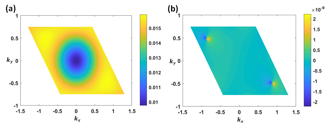
Refer to caption — Figure 1: (a) Phonon dispersion of graphene. The irreps for phonon modes at $\Gamma$ and $\mathbf{K}_{D}$ are labelled. Inset: BZ of graphene. (b) MBZ of TBG. (c) and (d) shows the momentum dependence of the normalized gap function $|\Delta_{\mathbf{k}}|$ for the inter-Chern-band $A_{1}$ singlet (or the $A_{2}$ triplet) channel and intra-Chern-band pairing 2D $E_{2}$ singlet channel, respectively. The inset in (c) shows the $|\Delta_{\mathbf{k}}|$ along the dashed line $k_{y}=0$ for both the inter-Chern-band (red) and intra-Chern-band (blue) channels. The momenta ${\bf\Gamma}_{M},\mathbf{K}_{M},{\bf M}_{M}$ are labelled in MBZ in (b) and (d).

Gap Equations and Self-consistent Solution of Pairing Channels - The linearized gap equation (LGE) for the attractive interaction (Electron- $K$ -Phonon Interaction In Twisted Bilayer Graphene) can be derived by evaluating $\langle\gamma_{-\mathbf{k}^{\prime}e_{Y_{2}}\eta s_{2}}\gamma_{\mathbf{k}^{\prime}e_{Y_{1}}-\eta s_{1}}\rangle$ in Eq. (9) and expanding it to linear order of the gap function. In the chiral flat band limit, e.g. the band width is much smaller than the critical temperature $T_{c}$ , the LGE is derived as

2k_{B}T\Delta^{\eta,SM}_{\mathbf{k};e_{Y_{1}}e_{Y_{2}}}=\frac{1}{N_{M}}\sum_{\mathbf{k}^{\prime}}V^{\eta e_{Y_{1}}e_{Y_{2}}}_{\mathbf{k},\mathbf{k}^{\prime}}\Delta^{-\eta,SM}_{\mathbf{k}^{\prime};e_{Y_{1}}e_{Y_{2}}}.

(10)

This is eigen-equation problem for the matrix $V^{\eta e_{Y_{1}}e_{Y_{2}}}_{\mathbf{k},\mathbf{k}^{\prime}}$ : the $T_{c}$ is determined by the largest eigen-value and the symmetry of the gap function is determined by that of its eigenvector. As mentioned, the only two independent components of the $V$ -function (complex $V^{+++}_{\mathbf{k},\mathbf{k}^{\prime}}$ and real $V^{++-}_{\mathbf{k},\mathbf{k}^{\prime}}$ ) leads to two independent LGEs for the intra- and inter-Chern-band channels, respectively. The form of the LGE suggests that all the gap functions are doubly degenerate at $T_{c}$ in the flat-band limit. They belong either to two degenerate 1D irreps or one 2D irrep. We first numerically solve these two LGEs from Eq. (358), and find the forms of the gap functions with the largest eigen-values, as shown in Fig. 1. Our numerical calculations show $k_{B}T_{c}\sim 0.21meV$ for the inter-Chern-band channel, slightly larger than $k_{B}T_{c}\sim 0.16meV$ for the intra-Chern-band channel. For the inter-Chern-band channels, the gap function is almost a constant in Fig. 1a, featuring a fully gapped s-wave pairing with even $\hat{C}_{2z}$ -parity ( $A_{1}$ or $A_{2}$ irrep). In the chiral flat-band limit, spin singlet and triplet pairings are degenerate, as required by the continuous $U(2)\times U(2)$ spin symmetry (SM Sec.VI.E sm2). Including kinetic energy splits this degeneracy and makes the spin singlet $A_{1}$ irrep channel to have the highest $T_{c}$ . For the intra-Chern-band channel, one can see nodes appear at the $\Gamma_{M}$ in Fig. 1b. As our previous symmetry analysis shows that the gap function should have nodes at $\mathbf{K}_{M}$ for the 1D irrep ( $A_{1,2},B_{1,2}$ ) and $\Gamma_{M}$ for the 2D irrep ( $E_{1,2}$ ), numerical results should correspond to a 2D irrep. Numerically analyzing the symmetry property of the gap function suggests that the intra-Chern-band channel belongs to the 2D $E_{2}$ irrep with spin singlet. Full numerical results are discussed in SM Sec.VI.H.2 and 3 sm2.

Our results for the intra-Chern-band channels reveal a d-wave character of the gap. Using the heavy fermion formalism of TBG Song and Bernevig 2022; liu, we analytically obtain $V^{\eta,e_{Y},e_{Y}}_{\mathbf{k},\mathbf{k}^{\prime}}$ :

\displaystyle V^{\eta,e_{Y},e_{Y}}_{\mathbf{k},\mathbf{k}^{\prime}}=U^{*}_{e_{Y},\mathbf{k}}U_{e_{Y},\mathbf{k}^{\prime}};\;\;U_{e_{Y},\mathbf{k}}=\frac{\sqrt{V_{0}}}{k^{2}+b^{2}}k_{e_{Y}}^{2},

(11)

with $k_{e_{Y}}=k_{x}+ie_{Y}k_{y}$ ( $e_{Y}=\pm$ ). This interaction allows us to solve the LGE analytically to obtain the $T_{c}$ ,

k_{B}T_{c}=\frac{\tilde{V}_{0}}{2},\;\;\tilde{V}_{0}=\frac{1}{N_{M}}\sum_{\mathbf{k}}V_{0}\frac{k^{4}}{(k^{2}+b^{2})^{2}},

(12)

where $V_{0}$ and $b$ are material dependent parameters. The corresponding self-consistent gap function takes the d-wave form

\displaystyle\left(\begin{array}[]{c}\Delta^{+,00}_{\mathbf{k},e_{Y}e_{Y}}\\ \Delta^{-,00}_{\mathbf{k},e_{Y}e_{Y}}\end{array}\right)=\Delta_{e_{Y}}\frac{k_{-e_{Y}}^{2}}{k^{2}+b^{2}}\left(\begin{array}[]{c}1\\ 1\end{array}\right)

with $e_{Y}=\pm$ and $\Delta_{e_{Y}}$ a parameter to be determined. Time reversal, if exists, requires $\left(\Delta^{-,00}_{\mathbf{k};--},\Delta^{+,00}_{\mathbf{k};--}\right)=\left(\Delta^{+,00}_{\mathbf{k};++},\Delta^{-,00}_{\mathbf{k};++}\right)^{*}$ . The d-wave nature of the gap function suggests the possibility of the nodal superconductivity. However, one should note that the single-particle Hamiltonian is not diagonal in the Chern-band basis. The Bogoliubov-de Gennes (BdG) spectrum must be checked with kinetic energy added. The BdG Hamiltonian for the intra-Chern-band pairing is block diagonal and one block $\mathcal{H}_{BdG}^{+,+}$ on the basis $(\gamma^{\dagger}_{\mathbf{k},e_{Y}=\pm,+,s=\uparrow},\gamma_{-\mathbf{k},e_{Y}=\pm,-,s=\downarrow})$ reads

\displaystyle H_{BdG}^{+,+}(\mathbf{k})=\begin{pmatrix}h_{+}(\mathbf{k})&\Delta^{+}_{\mathbf{k}}\\ (\Delta^{+}_{\mathbf{k}})^{\dagger}&-h_{-}^{\star}(-\mathbf{k})\end{pmatrix}

(18)

with $h_{\eta}(\mathbf{k})=(d_{0,\eta}(\mathbf{k})-\mu)\zeta^{0}+d_{x,\eta}(\mathbf{k})\zeta^{x}$ and $\Delta^{+}_{\mathbf{k}}=Diag[\Delta^{+,00}_{\mathbf{k},++},\Delta^{+,00}_{\mathbf{k},--}]$ . Here $d_{0,\eta}(\mathbf{k})=(\epsilon_{+,\eta}(\mathbf{k})+\epsilon_{-,\eta}(\mathbf{k}))/2$ and $d_{x,\eta}(\mathbf{k})=(\epsilon_{+,\eta}(\mathbf{k})-\epsilon_{-,\eta}(\mathbf{k}))/2$ , where $\epsilon_{\pm,\eta}(\mathbf{k})$ are the eigen-energies for the two low-energy flat bands (per valley per spin) of the BM model ${\hat{H}}_{\rm el}$ (2). The corresponding energy spectrum can possess nodes when the pairing amplitudes of two Chern-band channels are equal, $|\Delta_{e_{Y}=+}|=|\Delta_{e_{Y}=-}|=\Delta_{0}$ , which corresponds to the Euler pairing discussed in Ref.Yu et al. 2022b; Yu et al. 2022a. Point nodes appear at the location defined by two conditions (1) $\cos((\Phi_{\mathbf{k},-}-\Phi_{\mathbf{k},+})/2)=0$ , where $\Phi_{\mathbf{k},e_{Y}}=\varphi_{e_{Y}}-2e_{Y}\theta_{\mathbf{k}}$ with $\Delta_{e_{Y}}=\Delta_{0}e^{i\varphi_{e_{Y}}}$ and $k_{e_{Y}}=ke^{ie_{Y}\theta_{\mathbf{k}}}$ ; and (2) $d_{x,\mathbf{k}}^{2}=(d_{0,\mathbf{k}}-\mu)^{2}+\Delta_{0,\mathbf{k}}^{2}$ with $\Delta_{0,\mathbf{k}}=\Delta_{0}\frac{k^{2}}{k^{2}+b^{2}}$ , as discussed in SM Sec.VI.H.5 sm2. The first condition determines the momentum angle for the nodes while the second gives the momentum amplitude, thus together fixing the location of point nodes in the 2D momentum space. We next solve the self-consistent gap equation at zero temperature for the interaction form (414). With the gap function ansatz $\Delta_{\mathbf{k};e_{Y}}=\Delta_{e_{Y}}\frac{k^{2}_{-e_{Y}}}{k^{2}+b^{2}}$ , we find a self-consistent gap equation

\Delta_{e_{Y}}=\frac{V_{0}}{N_{M}}\sum_{\mathbf{k}^{\prime},e_{Y_{1}}}\frac{{k^{\prime}}^{2}_{e_{Y}}}{k^{\prime 2}+b^{2}}u_{-\mathbf{k}^{\prime},e_{Y}e_{Y_{1}}}w^{*}_{-\mathbf{k}^{\prime},e_{Y}e_{Y_{1}}},

(19)

where $\psi_{\mathbf{k},e_{Y_{1}}}=(u_{\mathbf{k},\pm,e_{Y_{1}}},w_{\mathbf{k},\pm e_{Y_{1}}})$ ( $e_{Y_{1}}=\pm$ ) are the eigen-wave functions with the positive eigen-energies of the BdG Hamiltonian $H_{BdG}^{+,+}(\mathbf{k})$ (18). Fig. 2A shows the chemical potential dependence of the gap functions and the condensation energy. The Euler pairing $|\Delta_{+}|=|\Delta_{-}|$ is always energetically favored for a non-flat band width $\sim 0.3meV$ , quite different from chiral d-wave pairing in doped graphene Black-Schaffer and Honerkamp 2014; Nandkishore et al. 2012; Wu 2019. For the chemical potential $\mu$ below $0.1meV$ , a nodal superconductor phase with four point nodes (Fig. 2B) located at the positions determined by two conditions discussed above Yu et al. 2022a. With increasing $\mu$ , four nodes move towards $\Gamma_{M}$ and eventually a gapped superconductor phase (Fig. 2C) appears for $\mu>0.1meV$ .

The energy scale of the Coulomb interaction in TBG is $\sim 24meV$ Bernevig et al. 2021, much larger than the estimated energy scale of e-K-ph mediated attractive interaction $\sim 0.3meV$ not. Near the Van-Hove singularities of flat bands, the screening can significantly reduce the Coulomb interaction to a similar order as e-K-ph mediated interaction due to the large DOS (SM Sec.VI.H.7 sm2), thus making superconductivity from this mechanism possible. If, however, the DOS is that of the Hartree-Fock bands of correlated insulators, the screening might not be enough to reduce the Coulomb interaction. Hence, superconductivity from this $K$ -phonon flat bare band mechanism could appear only when the correlated insulator states are suppressed.

Conclusion - In conclusion, we develop a theory for the projected e-K-ph interaction of the flat bands and the resulting superconductor pairing channels in TBG. We find the inter-Chern-band s-wave singlet pairing and the intra-Chern-band d-wave nematic singlet pairing have highest $T_{c}$ , and the $T_{c}$ of inter-Chern-band channel is slightly higher than the intra-Chen-band channel. The intra-Chen-band channel can have nodes in a large parameter regime. From the estimate of the screened Coulomb interaction, we argue that this mechanism requires the correlated insulators to be suppressed.

Acknowledgement – We would like to acknowledge Biao Lian, Xi Dai and Zhida Song for the helpful discussion. B.A.B.’s heavy fermion in twisted bilayer research was supported by the DOE Grant No. DE-SC0016239. BAB’s sabbatical support also comes from the Simons Investigator Grant No. 404513, the Gordon and Betty Moore Foundation through Grant No.GBMF8685 towards the Princeton theory program, the Gordon and Betty Moore Foundation’s EPiQS Initiative (Grant No. GBMF11070), Office of Naval Research (ONR Grant No. N00014-20-1-2303), and the European Research Council (ERC) under the European Union’s Horizon 2020 research and innovation program (grant agreement no. 101020833). CXL also acknowledges the support through the Penn State MRSEC–Center for Nanoscale Science via NSF award DMR-2011839. AY acknowledges support from the Gordon and Betty Moore Foundation’s EPiQS initiative grant GBMF9469, DOE- BES grant DE-FG02-07ER46419, NSF-DMR-1904442, ARO MURI (W911NF-21-2-0147), and ONR N00012- 21-1-2592. CXL and AY also acknowledges the support from the NSF-MERSEC (Grant No. MER- SEC DMR 2011750). YLC acknowledges the support from the Oxford-ShanghaiTech collaboration project and the Shanghai Municipal Science and Technology Major Project (grant 2018SHZDZX02).

References

Cao et al. (2018a) Y. Cao, V. Fatemi, A. Demir, S. Fang, S. L. Tomarken, J. Y. Luo, J. D. Sanchez-Yamagishi, K. Watanabe, T. Taniguchi, E. Kaxiras, et al., Nature 556, 80 (2018a).
Cao et al. (2018b) Y. Cao, V. Fatemi, S. Fang, K. Watanabe, T. Taniguchi, E. Kaxiras, and P. Jarillo-Herrero, Nature 556, 43 (2018b).
Lu et al. (2019) X. Lu, P. Stepanov, W. Yang, M. Xie, M. A. Aamir, I. Das, C. Urgell, K. Watanabe, T. Taniguchi, G. Zhang, et al., Nature 574, 653 (2019).
Codecido et al. (2019) E. Codecido, Q. Wang, R. Koester, S. Che, H. Tian, R. Lv, S. Tran, K. Watanabe, T. Taniguchi, F. Zhang, et al., Science Advances 5, eaaw9770 (2019).
Yankowitz et al. (2019) M. Yankowitz, S. Chen, H. Polshyn, Y. Zhang, K. Watanabe, T. Taniguchi, D. Graf, A. F. Young, and C. R. Dean, Science 363, 1059 (2019).
Cao et al. (2021) Y. Cao, D. Rodan-Legrain, J. M. Park, N. F. Yuan, K. Watanabe, T. Taniguchi, R. M. Fernandes, L. Fu, and P. Jarillo-Herrero, science 372, 264 (2021).
Oh et al. (2021) M. Oh, K. P. Nuckolls, D. Wong, R. L. Lee, X. Liu, K. Watanabe, T. Taniguchi, and A. Yazdani, Nature 600, 240 (2021).
Liu et al. (2021) X. Liu, Z. Wang, K. Watanabe, T. Taniguchi, O. Vafek, and J. Li, Science 371, 1261 (2021).
Saito et al. (2020) Y. Saito, J. Ge, K. Watanabe, T. Taniguchi, and A. F. Young, Nature Physics 16, 926 (2020).
Arora et al. (2020) H. S. Arora, R. Polski, Y. Zhang, A. Thomson, Y. Choi, H. Kim, Z. Lin, I. Z. Wilson, X. Xu, J.-H. Chu, et al., Nature 583, 379 (2020).
Andrei and MacDonald (2020) E. Y. Andrei and A. H. MacDonald, Nature materials 19, 1265 (2020).
Liu and Dai (2021) J. Liu and X. Dai, Nature Reviews Physics 3, 367 (2021).
Kwan et al. (2021) Y. H. Kwan, G. Wagner, T. Soejima, M. P. Zaletel, S. H. Simon, S. A. Parameswaran, and N. Bultinck, Physical Review X 11, 041063 (2021).
Nuckolls et al. (2023) K. P. Nuckolls, R. L. Lee, M. Oh, D. Wong, T. Soejima, J. P. Hong, D. Călugăru, J. Herzog-Arbeitman, B. A. Bernevig, K. Watanabe, et al., arXiv preprint arXiv:2303.00024 (2023).
Călugăru et al. (2022) D. Călugăru, N. Regnault, M. Oh, K. P. Nuckolls, D. Wong, R. L. Lee, A. Yazdani, O. Vafek, and B. A. Bernevig, Physical review letters 129, 117602 (2022).
Kang et al. (2021) J. Kang, B. A. Bernevig, and O. Vafek, Physical review letters 127, 266402 (2021).
Kang and Vafek (2018) J. Kang and O. Vafek, Physical Review X 8, 031088 (2018).
Kang and Vafek (2019) J. Kang and O. Vafek, Physical review letters 122, 246401 (2019).
Vafek and Kang (2020) O. Vafek and J. Kang, Physical Review Letters 125, 257602 (2020).
Khalaf et al. (2021) E. Khalaf, S. Chatterjee, N. Bultinck, M. P. Zaletel, and A. Vishwanath, Science advances 7, eabf5299 (2021).
Khalaf et al. (2022) E. Khalaf, P. Ledwith, and A. Vishwanath, Physical Review B 105, 224508 (2022).
Po et al. (2018) H. C. Po, L. Zou, A. Vishwanath, and T. Senthil, Physical Review X 8, 031089 (2018).
You and Vishwanath (2019) Y.-Z. You and A. Vishwanath, npj Quantum Materials 4, 1 (2019).
Lian et al. (2019) B. Lian, Z. Wang, and B. A. Bernevig, Physical review letters 122, 257002 (2019).
Wu et al. (2018) F. Wu, A. H. MacDonald, and I. Martin, Physical review letters 121, 257001 (2018).
Wu (2019) F. Wu, Physical Review B 99, 195114 (2019).
Wu et al. (2019) F. Wu, E. Hwang, and S. D. Sarma, Physical Review B 99, 165112 (2019).
Wu and Sarma (2019) F. Wu and S. D. Sarma, Physical Review B 99, 220507 (2019).
Chichinadze et al. (2020) D. V. Chichinadze, L. Classen, and A. V. Chubukov, Physical Review B 101, 224513 (2020).
Fernandes and Fu (2021) R. M. Fernandes and L. Fu, Physical review letters 127, 047001 (2021).
Wang et al. (2021) Y. Wang, J. Kang, and R. M. Fernandes, Physical Review B 103, 024506 (2021).
Yu et al. (2022a) J. Yu, M. Xie, F. Wu, and S. D. Sarma, arXiv preprint arXiv:2202.02353 (2022a).
Sharma et al. (2020) G. Sharma, M. Trushin, O. P. Sushkov, G. Vignale, and S. Adam, Physical Review Research 2, 022040 (2020).
Isobe et al. (2018) H. Isobe, N. F. Yuan, and L. Fu, Physical Review X 8, 041041 (2018).
Roy and Juričić (2019) B. Roy and V. Juričić, Physical Review B 99, 121407 (2019).
Peltonen et al. (2018) T. J. Peltonen, R. Ojajärvi, and T. T. Heikkilä, Physical Review B 98, 220504 (2018).
Kennes et al. (2018) D. M. Kennes, J. Lischner, and C. Karrasch, Physical Review B 98, 241407 (2018).
Gonzalez and Stauber (2019) J. Gonzalez and T. Stauber, Physical review letters 122, 026801 (2019).
Cea and Guinea (2021) T. Cea and F. Guinea, Proceedings of the National Academy of Sciences 118, e2107874118 (2021).
Shavit et al. (2021) G. Shavit, E. Berg, A. Stern, and Y. Oreg, Physical Review Letters 127, 247703 (2021).
Liu et al. (2018) C.-C. Liu, L.-D. Zhang, W.-Q. Chen, and F. Yang, Physical review letters 121, 217001 (2018).
Fidrysiak et al. (2018) M. Fidrysiak, M. Zegrodnik, and J. Spałek, Physical Review B 98, 085436 (2018).
Chou et al. (2019) Y.-Z. Chou, Y.-P. Lin, S. D. Sarma, and R. M. Nandkishore, Physical Review B 100, 115128 (2019).
Kozii et al. (2019) V. Kozii, H. Isobe, J. W. Venderbos, and L. Fu, Physical Review B 99, 144507 (2019).
(45) Cheng Chen, Kevin P. Nuckolls, Shuhan Ding, Wangqian Miao, Dillon Wong, Myungchul Oh, Ryan L. Lee, Shanmei He, Cheng Peng, Ding Pei, Yiwei Li, Shihao Zhang, Jianpeng Liu, Zhongkai Liu, Chris Jozwiak, Aaron Bostwick, Eli Rotenberg, Xi Dai, Chaoxing Liu, B. Andrei Bernevig, Yao Wang, Ali Yazdani, Yulin Chen, Strong Intervalley Electron-Phonon Coupling in Magic-Angle Twisted Bilayer Graphene, submitted.
Song and Bernevig (2022) Z.-D. Song and B. A. Bernevig, Physical Review Letters 129, 047601 (2022).
Călugăru et al. (2023) D. Călugăru, M. Borovkov, L. L. Lau, P. Coleman, Z.-D. Song, and B. A. Bernevig, arXiv preprint arXiv:2303.03429 (2023).
Hu et al. (2023a) H. Hu, G. Rai, L. Crippa, J. Herzog-Arbeitman, D. Călugăru, T. Wehling, G. Sangiovanni, R. Valenti, A. Tsvelik, and B. Bernevig, arXiv preprint arXiv:2301.04673 (2023a).
Hu et al. (2023b) H. Hu, B. A. Bernevig, and A. M. Tsvelik, arXiv preprint arXiv:2301.04669 (2023b).
Lau and Coleman (2023) L. L. Lau and P. Coleman, arXiv preprint arXiv:2303.02670 (2023).
Datta et al. (2023) A. Datta, M. J. Calderon, A. Camjayi, and E. Bascones, arXiv preprint arXiv:2301.13024 (2023).
Yu et al. (2023) J. Yu, M. Xie, B. A. Bernevig, and S. D. Sarma, arXiv preprint arXiv:2301.04171 (2023).
Chou and Sarma (2022) Y.-Z. Chou and S. D. Sarma, arXiv preprint arXiv:2211.15682 (2022).
Zhou and Song (2023) G.-D. Zhou and Z.-D. Song, arXiv preprint arXiv:2301.04661 (2023).
(55) See Supplemental Material at [URL] for details of the derivations of electron-phonon interaction in graphene and its projection to the flat bands of twisted bilayer graphene, symmetry analysis of phonon-mediated electron-electron interaction and irreducible superconductor pairing channels, the linearized and T=0 gap equations, the superconductor ground state energy and the Coulomb screening effect.
Bistritzer and MacDonald (2011) R. Bistritzer and A. H. MacDonald, Proceedings of the National Academy of Sciences 108, 12233 (2011).
Bernevig et al. (2021) B. A. Bernevig, Z.-D. Song, N. Regnault, and B. Lian, Physical Review B 103, 205413 (2021).
Song et al. (2021) Z.-D. Song, B. Lian, N. Regnault, and B. A. Bernevig, Physical Review B 103, 205412 (2021).
Neto et al. (2009) A. C. Neto, F. Guinea, N. M. Peres, K. S. Novoselov, and A. K. Geim, Reviews of modern physics 81, 109 (2009).
Sahoo and Mishra (2012) R. Sahoo and R. R. Mishra, Journal of Experimental and Theoretical Physics 114, 805 (2012).
Thingstad et al. (2020) E. Thingstad, A. Kamra, J. W. Wells, and A. Sudbø, Physical Review B 101, 214513 (2020).
Maultzsch et al. (2004) J. Maultzsch, S. Reich, C. Thomsen, H. Requardt, and P. Ordejón, Physical review letters 92, 075501 (2004).
Mohr et al. (2007) M. Mohr, J. Maultzsch, E. Dobardžić, S. Reich, I. Milošević, M. Damnjanović, A. Bosak, M. Krisch, and C. Thomsen, Physical Review B 76, 035439 (2007).
(64) Liu, Chao-Xing and Bernevig, B Andrei, in preparation.
Schrieffer and Wolff (1966) J. R. Schrieffer and P. A. Wolff, Physical Review 149, 491 (1966).
Bultinck et al. (2020) N. Bultinck, E. Khalaf, S. Liu, S. Chatterjee, A. Vishwanath, and M. P. Zaletel, Physical Review X 10, 031034 (2020).
Yu et al. (2022b) J. Yu, Y.-A. Chen, and S. D. Sarma, Physical Review B 105, 104515 (2022b).
Black-Schaffer and Honerkamp (2014) A. M. Black-Schaffer and C. Honerkamp, Journal of Physics: Condensed Matter 26, 423201 (2014).
Nandkishore et al. (2012) R. Nandkishore, L. S. Levitov, and A. V. Chubukov, Nature Physics 8, 158 (2012).
(70) Note that our calculation is performed in the chiral limit, so we may underestimate the electron-phonon coupling strength.
Song et al. (2019) Z. Song, Z. Wang, W. Shi, G. Li, C. Fang, and B. A. Bernevig, Physical review letters 123, 036401 (2019).
Tarnopolsky et al. (2019) G. Tarnopolsky, A. J. Kruchkov, and A. Vishwanath, Physical review letters 122, 106405 (2019).
Ahn et al. (2019) J. Ahn, S. Park, and B.-J. Yang, Physical Review X 9, 021013 (2019).
Po et al. (2019) H. C. Po, L. Zou, T. Senthil, and A. Vishwanath, Physical Review B 99, 195455 (2019).
Savary et al. (2017) L. Savary, J. Ruhman, J. W. Venderbos, L. Fu, and P. A. Lee, Physical Review B 96, 214514 (2017).
Sigrist and Ueda (1991) M. Sigrist and K. Ueda, Reviews of Modern physics 63, 239 (1991).

Supplementary Material for ”Electron- $K$ -Phonon Interaction In Twisted Bilayer Graphene”

I Notation

In this section, we will first describe our notations for the whole paper. We denote ${\bf a}_{1}^{l},{\bf a}_{2}^{l}$ as the un-strained, microscopic lattice vectors of the graphene layer $l$ ( $l=\pm$ for the top and bottom layers), while ${\bf G}_{1,2}^{l}$ are the corresponding reciprocal lattice vectors. ${\bf G}_{a}^{l}\cdot{\bf a}_{b}^{l}=2\pi\delta_{ab}$ . In the layer $l$ , there are two sub-lattice positions ${\bf\tau}_{A}^{l},{\bf\tau}_{B}^{l}$ . We assume the graphene layer $l$ is rotated by an in-plane angle $l\theta/2$ followed by a shift $l\frac{l_{0}}{2}\hat{z}$ along the z direction, so any vector ${\bf v}^{l}$ is related to the un-rotated vector ${\bf v}$ by ${\bf v}^{l}=\hat{R}^{l}_{\theta/2}{\bf v}+l\frac{l_{0}}{2}\hat{z}=l\frac{\theta}{2}\hat{z}\times{\bf v}+l\frac{l_{0}}{2}\hat{z}$ , where $\hat{R}^{l}_{\theta/2}$ labels the rotation operator, $\hat{z}$ is the out-of-plane unit vector and $l_{0}$ is the equilibrium distance between two graphene layers. Thus, we only need to give the values of all the un-rotated vectors below. Two primitive lattice vectors are ${\bf a}_{1}=a_{0}(\frac{-1}{2},\frac{\sqrt{3}}{2},0)$ and ${\bf a}_{2}=-a_{0}(\frac{1}{2},\frac{\sqrt{3}}{2},0)$ , where $a_{0}=2.46\AA$ is the lattice constant. The two primitive reciprocal lattice vectors spanning the Brillouin zone (BZ) are

{\bf G}_{1}=\frac{4\pi}{\sqrt{3}a_{0}}(-\frac{\sqrt{3}}{2},\frac{1}{2});\;\;{\bf G}_{2}=\frac{4\pi}{\sqrt{3}a_{0}}(-\frac{\sqrt{3}}{2},-\frac{1}{2}).

(20)

Since the Fermi surface in graphene is around two $K$ -valley, we also label them as $\eta\mathbf{K}_{D}$ with $\mathbf{K}_{D}=\frac{4\pi}{3a_{0}}(1,0)$ and $\eta=\pm$ . The atoms are at positions

{\bf\tau}_{A}=\frac{a_{0}}{2}(1,-\frac{1}{\sqrt{3}}),\;\;{\bf\tau}_{B}=\frac{a_{0}}{2}(1,\frac{1}{\sqrt{3}}).

(21)

For two layers $l=\pm$ , the atoms on position $\alpha=A,B$ in the top/bottom later reside at

{\bf R}^{l}_{\alpha}=\hat{R}_{\theta/2}^{l}{\bf R}+l\frac{l_{0}}{2}\hat{z}+{\bf\tau}_{\alpha}^{l}={\bf R}^{l}+{\bf\tau}_{\alpha}^{l}

(22)

where ${\bf R}=m{\bf a}_{1}+n{\bf a}_{2}$ is a unit cell vector.

The hopping between two atomic centers at a distance $r$ is

\displaystyle t({\bf r}_{\parallel},z)=V_{pp\pi}(1-(\frac{{\bf r}\cdot\hat{z}}{r})^{2})e^{-(r-\frac{a}{\sqrt{3}})/r_{0}}+V_{pp\sigma}(\frac{{\bf r}\cdot\hat{z}}{r})^{2}e^{-\frac{r-l_{0}}{r_{0}}}

(23)

where ${\bf r}_{\parallel}=(x,y)$ , $r_{0}$ characterizes the decaying length of atomic orbitals of carbon atoms, $a=a_{0}/\sqrt{3}$ is the distance between the $A$ and $B$ atoms, and $V_{pp\pi}$ and $V_{pp\sigma}$ are the hybridization parameters of $\pi$ and $\sigma$ bonds. We performed the Fourier transform to the in-plane coordinate of $t({\bf r}_{\parallel},z)$ ,

t_{{\bf q},z}=\frac{1}{S_{0}}\int d^{2}{\bf r}_{\parallel}e^{-i{\bf q}\cdot{\bf r}_{\parallel}}t({\bf r}_{\parallel},z)

(24)

where $S_{0}$ is the unit cell area.

In the discussion below, we mainly focus on the in-plane hopping term, and direct calculation gives

t_{{\bf q},0}=\frac{V_{pp\pi}e^{\frac{a_{0}}{\sqrt{3}r_{0}}}}{S_{0}}\frac{2\pi r_{0}^{2}}{(1+(qr_{0})^{2})^{3/2}}

(25)

In the calculation we have used

r_{0}=0.184a_{0};\;V_{pp\pi}=-2.7eV;\;S_{0}=\frac{\sqrt{3}a_{0}^{2}}{2};\;|\mathbf{K}_{D}|=1.7028\AA^{-1}

(26)

In the presence of a phonon field, the atom position should include the displacement field ${\bf u}^{l}({\bf R}^{l}_{\alpha})$ as

{\bf R}_{\alpha}^{l}={\bf R}^{l}+{\bf\tau}_{\alpha}^{l}\rightarrow\tilde{\bf R}_{\alpha}^{l}={\bf R}^{l}+{\bf\tau}_{\alpha}^{l}+{\bf u}^{l}({\bf R}^{l}_{\alpha})

(27)

where

{\bf u}^{l}({\bf R}^{l}+\tau_{\alpha}^{l})=\frac{1}{\sqrt{N_{G}}}\sum_{\bf p}{\bf u}_{\bf p}^{l,\alpha}e^{i{\bf p}\cdot({\bf R}^{l}+\tau_{\alpha}^{l})}

(28)

where the sum over ${\bf p}$ extends of the graphene BZ and the $N_{G}$ are the total number of atomic unit cells in graphene. Another important property of the phonon field is its periodic gauge. With the form of inversion Fourier transform

\mathbf{u}_{\mathbf{q}}^{l,\alpha}=\frac{1}{\sqrt{N_{G}}}\sum_{\mathbf{R}}\mathbf{u}^{l}(\mathbf{R}^{l}+\tau_{\alpha}^{l})e^{-i\mathbf{q}\cdot(\mathbf{R}^{l}+\tau_{\alpha}^{l})},

(29)

we can see

\mathbf{u}^{\alpha}_{\mathbf{q}+\mathbf{G}}=e^{-i\mathbf{G}\cdot\tau_{\alpha}}\mathbf{u}^{l\alpha}_{\mathbf{q}}

(30)

which is called the ”periodic gauge”.

Here we only introduce our notation for the single layer graphene, and the notation for the Moiré lattice for twisted bilayer graphene (TBG) will be introduced in Sec. V.

II Electron-phonon interaction in a single layer graphene

On the basis states

\left|\psi_{{\bf p},\alpha}^{l}\right\rangle=\frac{1}{\sqrt{N_{G}}}\sum_{{\bf R}^{l}}e^{i{\bf p}\cdot({\bf R}^{l}+{\bf\tau}_{\alpha}^{l})}\left|\psi({\bf R}_{\alpha}^{l}+{\bf u}^{l}({\bf R}^{l}+{\bf\tau}_{\alpha}^{l})\right\rangle,

(31)

the matrix Hamiltonian between the momentum ${\bf p},{\bf p}^{\prime}$ in layers $a,b=1,2$ and orbitals $\alpha,\beta=A,B$ is given by

\displaystyle H_{ll^{\prime}}^{\alpha\alpha^{\prime}}({\bf pp}^{\prime})=\frac{1}{N_{G}}\sum_{{\bf R}^{l},{\bf R}^{l^{\prime}}}t(\tilde{\bf R}_{\alpha}^{l}-\tilde{\bf R}_{\alpha^{\prime}}^{l^{\prime}})e^{-i({\bf R}_{\alpha}^{l}\cdot{\bf p}-{\bf R}_{\alpha^{\prime}}^{l^{\prime}}\cdot{\bf p}^{\prime})}

(32)

H_{ll^{\prime}}^{\alpha\alpha^{\prime}}({\bf pp}^{\prime})=\frac{S_{0}}{(2\pi)^{2}N_{G}}\int d^{2}{\bf q}\left(\sum_{{\bf R}^{l},{\bf R}^{l^{\prime}}}e^{-i({\bf R}_{\alpha}^{l}\cdot({\bf p-q})-{\bf R}_{\alpha^{\prime}}^{l^{\prime}}\cdot({\bf p}^{\prime}-{\bf q}))}e^{i{\bf q}\cdot({\bf u}({\bf R}_{\alpha}^{l})-{\bf u}({\bf R}_{\alpha^{\prime}}^{l^{\prime}}))}\right)t({\bf q},z_{ll^{\prime}})

(33)

where $z_{ll^{\prime}}$ is the height difference between the layers $l$ and $l^{\prime}$ . In this section, we first discuss the electron-phonon (e-ph) interaction in the same layer $l=l^{\prime}$ , and may drop the layer index $l$ in some expressions for simplicity.

II.1 Zero Displacement

We have

\frac{1}{N_{G}}\sum_{{\bf R}^{l}}e^{-i{\bf R}^{l}\cdot({\bf p-q})}=\sum_{{\bf G}^{l}}\delta_{{\bf p-q},{\bf G}^{l}}

(34)

where ${\bf G}^{l}$ is a reciprocal lattice vector in the layer $l$ .

For the layer $l=l^{\prime}$ , we have (since $z_{ll}=0$ )

	$\displaystyle H_{0,ll}^{\alpha\alpha^{\prime}}({\bf pp}^{\prime})=\frac{S_{0}N_{G}}{(2\pi)^{2}}\int d^{2}{\bf q}\sum_{{\bf G}_{a}^{l},{\bf G}_{b}^{l}}\left(\delta_{{\bf p-q},-{\bf G}_{a}^{l}}\delta_{{\bf p^{\prime}-q},-{\bf G}_{b}^{l}}e^{-i{\bf G}_{b}^{l}\cdot{\bf\tau}_{\alpha^{\prime}}^{l}+i{\bf G}_{a}^{l}\cdot{\bf\tau}_{\alpha}^{l}}\right)t({\bf q},0)$
	$\displaystyle=\sum_{{\bf G}_{a}^{l},{\bf G}_{b}^{l}}\delta_{{\bf p}+{\bf G}_{a}^{l},{\bf p}^{\prime}+{\bf G}_{b}^{l}}e^{-i{\bf G}_{b}^{l}\cdot{\bf\tau}_{\alpha^{\prime}}^{l}+i{\bf G}_{a}^{l}\cdot{\bf\tau}_{\alpha}^{l}}t({\bf p+G}_{a}^{l},0)$		(35)

where ${\bf G}_{a}^{l}$ , ${\bf G}_{b}^{l}$ are two sets of reciprocal lattice vectors in the BZ of the layer $l$ . The summation in Eq. (35) respects the symmetries of the problem. When we restrict ${\bf p,p}^{\prime}$ to the same (first) BZ of graphene, we have $\delta_{{\bf p+G}_{a}^{l},{\bf p^{\prime}+G}_{b}^{l}}=\delta_{\bf p,p^{\prime}}\delta_{{\bf G}_{a}^{l},{\bf G}_{b}^{l}}$ and hence

H_{0ll}^{\alpha\alpha^{\prime}}({\bf pp}^{\prime})=\delta_{\bf p,p^{\prime}}\sum_{{\bf G}_{a}^{l}}e^{-i{\bf G}_{a}^{l}\cdot({\bf\tau}_{\alpha^{\prime}}^{l}-{\bf\tau}_{\alpha}^{l})}t({\bf p+G}_{a}^{l},0)

(36)

We then have the tight-binding Hamiltonian for the single layer graphene

t_{\bf p}^{\alpha\alpha^{\prime}}=\sum_{{\bf G}_{a}^{l}}e^{-i{\bf G}_{a}^{l}\cdot({\bf\tau}_{\alpha^{\prime}}^{l}-{\bf\tau}_{\alpha}^{l})}t({\bf p+G}_{a}^{l},0),

(37)

which has a node at the ${\bf K}_{D}$ point.

II.2 Finite Out of-Plane Displacement

For the out-of-plane displacement, we can use hopping $t({\bf q},z=u^{z}({\bf R}_{\alpha}^{l})-u^{z}({\bf R}_{\alpha}^{\prime l}))$ . With the small displacement approximation, we can linearize the expression in small $u$ , and sum over graphene lattice, leading to the intra-layer Hamiltonian

	$\displaystyle H_{\perp ll}^{\alpha\alpha^{\prime}}({\bf pp}^{\prime})=\frac{S_{0}}{(2\pi)^{2}N_{G}}\int d^{2}{\bf q}\left(\sum_{{\bf R}_{1}^{l},{\bf R}_{2}^{l}}e^{-i({\bf R}_{1\alpha}^{l}({\bf p-q})-{\bf R}_{2\alpha^{\prime}}^{l}({\bf p^{\prime}-q}))}(u^{z}({\bf R}_{\alpha}^{l})-u^{z}({\bf R}_{\alpha}^{\prime l}))\partial_{z}t({\bf q},z)\|_{z=0}\right)$
	$\displaystyle=\frac{1}{N^{1/2}_{G}}\sum_{{\bf p}_{1}\in BZ}\sum_{{\bf G}_{a}^{l},{\bf G}_{b}^{l}}e^{i(\tau_{\alpha}^{l}\cdot{\bf G}_{a}^{l}-\tau_{\alpha^{\prime}}^{l}\cdot{\bf G}_{b}^{l})}\delta_{{\bf p^{\prime}+p_{1}+G}_{b}^{l},{\bf p+G}_{a}^{l}}$
	$\displaystyle\left(u_{{\bf p}_{1}}^{zl,\alpha}\partial_{z}t({\bf G}_{a}^{l}+{\bf p-p_{1}},z)\|_{z=0}-u_{\bf p_{1}}^{zl,\alpha^{\prime}}\partial_{z}t({\bf G}_{b}^{l}+{\bf p^{\prime}+p_{1}},z)\|_{z=0}\right).$		(38)

One can show that

\frac{\partial t({\bf r},t)}{\partial z}|_{z=0}=0

(39)

and hence there is no out-of-plane phonon coupling to the graphene electrons (this will also be derived by symmetry), and thus

H_{\perp ll}^{\alpha\alpha^{\prime}}({\bf pp}^{\prime})=0

(40)

Thus, we only focus on in-plane phonon coupling below.

II.3 Finite In-Plane Displacement

For the in-plane displacement, we can use the Fourier transform form of the hopping term, $t({\bf q},z=0)$ . With the small displacement approximation, we can linearize ${\bf u}$ , and sum over graphene lattice, leading to the intra-layer Hamiltonian

	$\displaystyle H_{\parallel ll}^{\alpha\alpha^{\prime}}({\bf pp}^{\prime})=\frac{S_{0}}{(2\pi)^{2}N_{G}}\int d^{2}{\bf q}\left(\sum_{{\bf R}_{1}^{l},{\bf R}_{2}^{l}}e^{-i({\bf R}_{1\alpha}^{l}\cdot({\bf p-q})-{\bf R}_{2\alpha^{\prime}}^{l}({\bf p^{\prime}-q}))}i{\bf q}\cdot({\bf u}({\bf R}_{1\alpha}^{l})-{\bf u}({\bf R}_{2\alpha^{\prime}}^{l}))\right)t({\bf q},0)$
	$\displaystyle=\frac{S_{0}N^{1/2}_{G}}{(2\pi)^{2}}\int d^{2}{\bf q}\times t({\bf q},0)i{\bf q}\cdot$
	$\displaystyle\sum_{{\bf p}_{1}\in BZ}\sum_{{\bf G}_{a}^{l},{\bf G}_{b}^{l}}\left(\delta_{{\bf-p_{1}+p-q},-{\bf G}_{a}^{l}}\delta_{{\bf p^{\prime}-q},-{\bf G}_{b}^{l}}e^{i({\bf\tau}_{\alpha}^{l}\cdot{\bf G}_{a}^{l}-{\bf\tau}_{\alpha^{\prime}}^{l}\cdot{\bf G}_{b}^{l}))}{\bf u}_{{\bf p}_{1}}^{l,\alpha}-\delta_{{\bf p_{1}+p^{\prime}-q},-{\bf G}_{b}^{l}}\delta_{{\bf p-q},-{\bf G}_{a}^{l}}e^{i({\bf\tau}_{\alpha}^{l}\cdot{\bf G}_{a}^{l}-{\bf\tau}_{\alpha^{\prime}}^{l}\cdot{\bf G}_{b}^{l})}{\bf u}_{{\bf p}_{1}}^{l,\alpha^{\prime}}\right)$		(41)

where ${\bf G}_{a}^{l},{\bf G}_{b}^{l}$ are two sets of reciprocal lattice vectors in the the BZ of layer $l$ . Transforming the $\delta$ functions

	$\displaystyle\delta_{{\bf-p_{1}+p-q},-{\bf G}_{a}^{l}}\delta_{{\bf p^{\prime}-q},-{\bf G}_{b}^{l}}=\delta_{{\bf q},\frac{{\bf G}_{a}^{l}+{\bf G}_{b}^{l}+{\bf p+p^{\prime}-p}_{1}}{2}}\delta_{{\bf p^{\prime}+p}_{1}+{\bf G}_{b}^{l},{\bf p+G}_{a}^{l}}$
	$\displaystyle\delta_{{\bf p_{1}+p^{\prime}-q},-{\bf G}_{b}^{l}}\delta_{{\bf p-q},-{\bf G}_{a}^{l}}=\delta_{{\bf q},\frac{{\bf G}_{a}^{l}+{\bf G}_{b}^{l}+{\bf p+p^{\prime}+p_{1}}}{2}}\delta_{{\bf p^{\prime}+p_{1}+G}_{b}^{l},{\bf p+G}_{a}^{l}},$		(42)

we find the matrix elements of the intra-layer Hamiltonian,

	$\displaystyle H_{\parallel l}^{\alpha\alpha^{\prime}}({\bf pp}^{\prime})=\frac{1}{N^{1/2}_{G}}\sum_{{\bf p}_{1}\in BZ}\sum_{{\bf G}_{a}^{l},{\bf G}_{b}^{l}}e^{i({\bf\tau}_{\alpha}^{l}\cdot{\bf G}_{a}^{l}-{\bf\tau}_{\alpha^{\prime}}^{l}\cdot{\bf G}_{b}^{l})}\delta_{{\bf p^{\prime}+p_{1}+G}_{b}^{l},{\bf p+G}_{a}^{l}}$
	$\displaystyle\left(i\frac{{\bf G}_{a}^{l}+{\bf G}_{b}^{l}+{\bf p+p^{\prime}-p_{1}}}{2}\cdot{\bf u}_{{\bf p}_{1}}^{l,\alpha}t(\frac{{\bf G}_{a}^{l}+{\bf G}_{b}^{l}+{\bf p+p^{\prime}-p_{1}}}{2},0)-i\frac{{\bf G}_{a}^{l}+{\bf G}_{b}^{l}+{\bf p+p^{\prime}+p_{1}}}{2}\cdot{\bf u}_{{\bf p}_{1}}^{l,\alpha^{\prime}}t(\frac{{\bf G}_{a}^{l}+{\bf G}_{b}^{l}+{\bf p+p^{\prime}+p_{1}}}{2},0)\right)=$
	$\displaystyle=\frac{1}{N^{1/2}_{G}}\sum_{{\bf p}_{1}\in BZ}\sum_{{\bf G}_{a}^{l},{\bf G}_{b}^{l}}e^{i({\bf\tau}_{\alpha}^{l}\cdot{\bf G}_{a}^{l}-{\bf\tau}_{\alpha^{\prime}}^{l}\cdot{\bf G}_{b}^{l})}\delta_{{\bf p^{\prime}+p_{1}+G}_{b}^{l},{\bf p+G}_{a}^{l}}$
	$\displaystyle\left(i({\bf G}_{a}^{l}+{\bf p-p_{1}})\cdot{\bf u}_{{\bf p}_{1}}^{l,\alpha}t({\bf G}_{a}^{l}+{\bf p-p_{1}},0)-i({\bf G}_{b}^{l}+{\bf p^{\prime}+p_{1}})\cdot{\bf u}_{{\bf p}_{1}}^{l,\alpha^{\prime}}t({\bf G}_{b}^{l}+{\bf p^{\prime}+p_{1}},0)\right)$		(43)

It should be noted that ${\bf p}_{1}$ summation in the above expression is over one BZ. For convenience, we can choose it within the first BZ. From the $\delta$ -function, we have ${\bf p_{1}}={\bf p+G}_{a}^{l}-{\bf p^{\prime}-G}_{b}^{l}$ , so if we keep the summation over ${\bf G}_{b}^{l}$ , only one ${\bf G}_{a}^{l}$ is allowed to make ${\bf p}_{1}$ in the first BZ. Actually the choice of ${\bf G}_{a}^{l}$ will not influence the results. To see that, let’s assume the choice of ${\bf G}_{a0}^{l}$ can make ${\bf p}_{10}={\bf p+G}_{a0}^{l}-{\bf p^{\prime}-G}_{b}^{l}$ within the first BZ, and now we consider another choice ${\bf G}_{a}^{l}={\bf G}_{a0}^{l}+\Delta{\bf G}^{l}$ , so ${\bf p_{1}=p+G}_{a}^{l}-{\bf p^{\prime}-G}_{b}^{l}={\bf p}_{10}+\Delta{\bf G}^{l}$ is outside the first BZ. For the first term in Eq. (43), we have

	$\displaystyle e^{i(\tau_{\alpha}^{l}\cdot{\bf G}_{a}^{l}-\tau_{\alpha^{\prime}}^{l}\cdot{\bf G}_{b}^{l})}i({\bf G}_{a}^{l}+{\bf p-p_{1}})\cdot{\bf u}_{{\bf p}_{1}}^{l,\alpha}t({\bf G}_{a}^{l}+{\bf p-p_{1}},0)$
	$\displaystyle=e^{i(\tau_{\alpha}^{l}\cdot({\bf G}_{a0}^{l}+\Delta{\bf G}^{l})-\tau_{\alpha^{\prime}}^{l}\cdot{\bf G}_{b}^{l})}i({\bf G}_{a0}^{l}+{\bf p-p_{10}})\cdot{\bf u}_{{\bf p}_{10}+\Delta{\bf G}^{l}}^{l,\alpha}t({\bf G}_{a0}^{l}+{\bf p-p_{10}},0)$
	$\displaystyle=e^{i(\tau_{\alpha}^{l}\cdot{\bf G}_{a0}^{l}-\tau_{\alpha^{\prime}}^{l}\cdot{\bf G}_{b}^{l})}i({\bf G}_{a0}^{l}+{\bf p-p}_{10})\cdot{\bf u}_{{\bf p}_{10}}^{l,\alpha}t({\bf G}_{a0}^{l}+{\bf p-p}_{10},0)$		(44)

where we have used the periodic gauge $\mathbf{u}^{l,\alpha}_{\mathbf{p}_{10}+\Delta\mathbf{G}^{l}}=e^{-i\tau_{\alpha}^{l}\cdot\Delta{\bf G}^{l}}{\bf u}_{\mathbf{p}_{10}}^{l,\alpha}$ . From the above expression, one can see that the first term in Eq. (43) remains the same if one changes from the summation over ${\bf p}_{10}$ to that over ${\bf p}_{1}$ . This means one just needs to pick one ${\bf G}_{a}^{l}$ (e.g. one possible choice ${\bf G}_{a}^{l}={\bf G}_{b}^{l}$ ), while which choice will not influence the results. Similar analysis can also be applied to the second term in Eq. (43).

Both in graphene and TBG, the electronic states with the energies around the Fermi energy is only close to the $\eta{\bf K}_{D}$ point where $\eta=\pm$ is the valley. Thus, one needs to expand the electron-phonon Hamiltonian around $\eta{\bf K}_{D}$ . The electron momenta $\mathbf{p}$ and $\mathbf{p}^{\prime}$ in Eq. (II.3) can be expanded around the same valley ( $\eta{\bf K}_{D}$ for a fixed $\eta$ ) or opposite valleys ( $\eta{\bf K}_{D}$ and $-\eta{\bf K}_{D}$ ), corresponding to intra-valley and inter-valley e-ph interaction, respectively. In this work, we focus on inter-valley e-ph interaction.

II.4 Inter-valley Electron-Phonon Interaction with In-plane Phonons

In this section, we choose $\mathbf{p}=\mathbf{k}+\eta\mathbf{K}_{D}$ , $\mathbf{p}^{\prime}=\mathbf{k}^{\prime}-\eta\mathbf{K}_{D}$ where $k,k^{\prime}\ll|\mathbf{K}_{D}|$ , and correspondingly, we also need to decompose the phonon momentum into a large value (the difference between the two valleys) and a small value around that,

\mathbf{p}_{1}=\mathbf{p}+\mathbf{P}_{1},;\;\;p\ll P_{1}

(45)

where $\mathbf{P}_{1}$ determines the major part of phonon momentum. The momentum $\delta$ -function in $H_{\parallel ll}^{\alpha\alpha^{\prime}}(\mathbf{p}\mathbf{p}^{\prime})$ becomes

\delta_{\mathbf{k}+\eta\mathbf{K}_{D}+\mathbf{G}_{a}^{l},\mathbf{k}^{\prime}-\eta\mathbf{K}_{D}+\mathbf{p}_{1}+\mathbf{G}_{b}^{l}}=\delta_{\mathbf{k},\mathbf{k}^{\prime}+\mathbf{p}}\delta_{2\eta K_{D}+\mathbf{G}_{a}^{l}-\mathbf{G}_{b}^{l},\mathbf{P}_{1}}.

(46)

For the momentum $\mathbf{p}$ in the first BZ, there are $3$ possible values for $\mathbf{P}_{1}$ momenta

\mathbf{P}_{1}=-\eta\mathbf{K}_{D};-\eta(\mathbf{K}_{D}+\mathbf{G}_{1});-\eta(\mathbf{K}_{D}+\mathbf{G}_{2}).

(47)

However, as discussed in Sec. II.3, the summation over $\mathbf{p}_{1}$ in the Hamiltonian (43) is within one BZ and the choice of different BZs will not influence the result due to the periodic gauge of the phonon modes. Thus, we make the choice of $\mathbf{P}_{1}=-\eta\mathbf{K}_{D}$ below, which corresponds to the K-phonon, and the Hamiltonian reads

	$\displaystyle H_{\parallel l}^{\eta\alpha,-\eta\alpha^{\prime}}(\mathbf{k}\mathbf{k}^{\prime})=\frac{i}{N^{1/2}_{G}}\sum_{\mathbf{G}_{a}^{l}}e^{i(\tau_{\alpha}^{l}-\tau_{\alpha^{\prime}}^{l})\cdot\mathbf{G}_{a}^{l}}e^{i\tau_{\alpha^{\prime}}^{l}\cdot(\mathbf{P}_{1}-2\eta\mathbf{K}_{D})}$
	$\displaystyle\left((\mathbf{G}_{a}^{l}+\eta\mathbf{K}_{D}+\mathbf{k}^{\prime}-\mathbf{P}_{1})\cdot\mathbf{u}_{\mathbf{P}_{1}+\mathbf{k}-\mathbf{k}^{\prime}}^{l,\alpha}t(\mathbf{G}_{a}^{l}+\eta\mathbf{K}_{D}+\mathbf{k}^{\prime}-\mathbf{P}_{1},0)-(\mathbf{G}_{a}^{l}+\eta\mathbf{K}_{D}+\mathbf{k})\cdot\mathbf{u}_{\mathbf{P}_{1}+\mathbf{k}-\mathbf{k}^{\prime}}^{l,\alpha^{\prime}}t(\mathbf{G}_{a}^{l}+\eta\mathbf{K}_{D}+\mathbf{k},0)\right)$
	$\displaystyle=\frac{i}{N^{1/2}_{G}}\sum_{\mathbf{G}_{a}^{l}}e^{i(\tau_{\alpha}^{l}-\tau_{\alpha^{\prime}}^{l})\cdot\mathbf{G}_{a}^{l}}\left((\mathbf{G}_{a}^{l}+2\eta\mathbf{K}_{D}+\mathbf{k}^{\prime})\cdot\mathbf{u}_{-\eta\mathbf{K}_{D}+\mathbf{k}-\mathbf{k}^{\prime}}^{l,\alpha}t(\mathbf{G}_{a}^{l}+2\eta\mathbf{K}_{D}+\mathbf{k}^{\prime},0)\right.$
	$\displaystyle\left.-(\mathbf{G}_{a}^{l}+\eta\mathbf{K}_{D}+\mathbf{k})\cdot\mathbf{u}_{-\eta\mathbf{K}_{D}+\mathbf{k}-\mathbf{k}^{\prime}}^{l,\alpha^{\prime}}t(\mathbf{G}_{a}^{l}+\eta\mathbf{K}_{D}+\mathbf{k},0)\right),$		(48)

where we have used

	$\displaystyle 3\mathbf{K}_{D}=\mathbf{G}_{1}+\mathbf{G}_{2}$
	$\displaystyle e^{i\tau_{A}\cdot(\mathbf{G}_{1}+\mathbf{G}_{2})}=e^{i\tau_{B}\cdot(\mathbf{G}_{1}+\mathbf{G}_{2})}=1.$		(49)

We next parameterize the above expression and define

	$\displaystyle\gamma_{0}=\sum_{\mathbf{G}_{a}}t(\mathbf{G}_{a}+\eta\mathbf{K}_{D},0),$
	$\displaystyle\gamma_{1}=\sum_{\mathbf{G}_{a}}(\widehat{\mathbf{G}_{a}+\eta\mathbf{K}_{D}})_{x}(\mathbf{G}_{a}+\eta\mathbf{K}_{D})_{x}\frac{\partial{t(\mathbf{q},0)}}{\partial q}\|_{q=\|\mathbf{K}_{D}+\eta\mathbf{G}_{a}\|},$		(50)

\gamma_{2}=\sum_{\mathbf{G}_{a}}e^{i(\tau_{A}-\tau_{B})\cdot\mathbf{G}_{a}}(\widehat{\mathbf{G}_{a}+\mathbf{K}_{D}})_{x}(\mathbf{G}_{a}+\mathbf{K}_{D})_{x}\frac{\partial{t(\mathbf{q},0)}}{\partial q}|_{q=|\mathbf{K}_{D}+\mathbf{G}_{a}|}

(51)

and

\gamma_{3}=2i\sum_{\mathbf{G}_{a}}e^{i(\tau_{A}-\tau_{B})\cdot\mathbf{G}_{a}}(\mathbf{G}_{a}+\mathbf{K}_{D})_{y}t(\mathbf{G}_{a}+\mathbf{K}_{D},0).

(52)

We also define the acoustic and optical basis for the displacement field as

\mathbf{u}_{\mathbf{p}}^{l,\alpha}=\mathbf{u}_{\mathbf{p}}^{l,ac}+(-1)^{\alpha}\mathbf{u}_{\mathbf{p}}^{l,op}

(53)

where we define $(-1)^{\alpha=A(B)}=-1(+1)$ .

With the above definitions, we can simplify the inter-valley e-ph Hamiltonian as

	$\displaystyle H_{\parallel l}^{\eta,-\eta}(\mathbf{k}\mathbf{k}^{\prime})=-\frac{i}{\sqrt{N_{G}}}(\gamma_{0}+\gamma_{1})(\mathbf{k}-\mathbf{k}^{\prime})\cdot(\mathbf{u}_{-\eta\mathbf{K}_{D}+\mathbf{k}-\mathbf{k}^{\prime}}^{l,ac}\sigma_{0}-\mathbf{u}_{-\eta\mathbf{K}_{D}+\mathbf{k}-\mathbf{k}^{\prime}}^{l,op}\sigma_{z})$
	$\displaystyle+\frac{1}{\sqrt{N_{G}}}\gamma_{3}\sigma_{x}(-u^{l,op}_{-\eta\mathbf{K}_{D}+\mathbf{k}-\mathbf{k}^{\prime},y}-i\eta u^{l,ac}_{-\eta\mathbf{K}_{D}+\mathbf{k}-\mathbf{k}^{\prime},x})$
	$\displaystyle+\frac{i}{\sqrt{N_{G}}}\gamma_{2}[(-(k_{x}-k^{\prime}_{x})\sigma_{x}+\eta(k_{y}+k^{\prime}_{y})\sigma_{y})u^{l,ac}_{-\eta\mathbf{K}_{D}+\mathbf{k}-\mathbf{k}^{\prime},x}+((k_{y}-k^{\prime}_{y})\sigma_{x}+\eta(k_{x}+k^{\prime}_{x})\sigma_{y})u^{l,ac}_{-\eta\mathbf{K}_{D}+\mathbf{k}-\mathbf{k}^{\prime},y}]$
	$\displaystyle+\frac{1}{\sqrt{N_{G}}}\gamma_{2}[((k_{x}+k^{\prime}_{x})\sigma_{y}+\eta(k_{y}-k_{y}^{\prime})\sigma_{x})u^{l,op}_{-\eta\mathbf{K}_{D}+\mathbf{k}-\mathbf{k}^{\prime},x}+(-(k_{y}+k^{\prime}_{y})\sigma_{y}+\eta(k_{x}-k_{x}^{\prime})\sigma_{x})u^{l,op}_{-\eta\mathbf{K}_{D}+\mathbf{k}-\mathbf{k}^{\prime},y}],$		(54)

where the Pauli matrix $\sigma$ is for the sublattice basis ( $(\sigma_{i})_{\alpha,\alpha^{\prime}}$ with $\alpha,\alpha^{\prime}=A,B$ ).

In addition, we also define

v_{F}=\left|\sum_{\mathbf{G}_{a}}e^{i\mathbf{G}_{a}\cdot(\tau_{A}-\tau_{B})}\widehat{(\mathbf{K}_{D}+\mathbf{G}_{a})}_{x}\frac{\partial{t(\mathbf{q},0)}}{\partial q}|_{q=|\mathbf{K}_{D}+\mathbf{G}_{a}|}\right|

(55)

for the Fermi velocity of graphene.

All these parameters can be numerically evaluated and their values are listed in Table (1) for both the $3$ $\mathbf{G}_{a}$ and for 2000 (infinite) $\mathbf{G}_{a}$ ’s. One can see a large difference for the obtained values for all the parameters when keeping only $3$ $\mathbf{G}_{a}$ , as compared to keeping 2000 (infinite) $\mathbf{G}_{a}$ ’s. For example, when keeping of order 2000 $G_{a}$ ’s, we find $\gamma_{1}=63.506$ and $\gamma_{0}=-61.4306$ , which almost cancel each other, and hence $\gamma=\gamma_{0}+\gamma_{1}=2.07565$ . For the first $3$ $\mathbf{G}_{a}$ ’s approximation, $\gamma_{0}=-22.7898$ and $\gamma_{1}=12.7393$ , and hence $\gamma=-10.0505$ , which is larger and of opposite sign as compared to keeping all $\mathbf{G}_{a}$ . Here $\gamma_{0},\gamma_{1}$ and $\gamma_{2}$ is in the unit of eV while $\gamma_{3}$ is in the unit of $eV/\AA$ .

	Infinite	3 Shells	3/Infinite
$v_{f}$	$5.229$	$7.3206$	$1.4$
$\gamma_{0}$	$-61.4306$	$-22.7898$	$0.371$
$\gamma_{1}$	$63.5062$	$12.7393$	$0.2006$
$\gamma=\gamma_{0}+\gamma_{1}$	$2.07565$	$-10.0505$	$-4.8421$
$\gamma_{2}$	$6.7281$	$6.3917$	$0.95$
$\gamma_{3}$	$-17.088$	$-37.5936$	$2.2$

Table 1: Table for all the parameters in the Hamiltonian (II.4). Here

\gamma_{0},\gamma_{1}

and

\gamma_{2}

is in the unit of eV while

\gamma_{3}

is in the unit of

eV/\AA

In the above Hamiltonian (II.4), the term in the second line ( $\gamma_{3}$ term) is zeroth order in $\mathbf{k}$ while all the other terms linearly depend on $\mathbf{k}$ . Thus, we below only keep the zeroth-order term for e-ph interaction for K-phonons.

II.4.1 Physical Meaning of the phonon Modes at $\mathbf{K}_{D}$

We now focus on the leading term of the inter-valley electron-phonon Hamiltonian

\displaystyle H=\frac{\gamma_{3}}{\sqrt{N_{G}}}\sum_{\mathbf{k},\mathbf{k}^{\prime},\eta,\alpha\beta}(-u^{l,op}_{-\eta\mathbf{K}_{D}+\mathbf{k}-\mathbf{k}^{\prime},y}-i\eta u^{l,ac}_{-\eta\mathbf{K}_{D}+\mathbf{k}-\mathbf{k}^{\prime},x})c^{\dagger}_{\mathbf{k}+\eta\mathbf{K}_{D},\alpha}(\sigma_{x})_{\alpha\beta}c_{\mathbf{k}^{\prime}-\eta\mathbf{K}_{D},\beta}

(56)

where the Hamiltonian is hermitian once the summation over $\eta$ is performed. We take the Fourier transform form of the phonon field

\displaystyle\mathbf{u}_{\alpha}(\mathbf{k}-\mathbf{k}^{\prime}-\eta\mathbf{K}_{D})=\frac{1}{\sqrt{N_{G}}}\sum_{\mathbf{R}}e^{i\eta\mathbf{K}_{D}\cdot(\mathbf{R}+\tau_{\alpha})}e^{-i(\mathbf{k}-\mathbf{k}^{\prime})\cdot(\mathbf{R}+\tau_{\alpha})}\mathbf{u}_{\alpha}(\mathbf{R}+\tau_{\alpha}).

(57)

We can see that the term $\eta\mathbf{K}_{D}\cdot\mathbf{R}$ is not periodic in $\mathbf{R}$ , and this problem can be fixed by enlarging the unit cell. By choosing $\mathbf{R}=n\mathbf{a}_{1}+m\mathbf{a}_{2}$ , we have

\mathbf{K}_{D}\cdot\mathbf{R}=-\frac{2\pi}{3}(m+n).

(58)

By choosing

m+n=3n_{1}+s\;\;\;

(59)

with $s=0,1,2$ and

\sum_{\mathbf{R}}=\sum_{m,n}=\sum_{n_{1},m,s},

(60)

We have

\mathbf{R}^{\prime}=3n_{1}\mathbf{a}_{1}+m(\mathbf{a}_{2}-\mathbf{a}_{1}),\;\;\mathbf{R}=\mathbf{R}^{\prime}+s\mathbf{a}_{1},

(61)

	$\displaystyle\mathbf{u}_{\alpha}(\mathbf{k}-\mathbf{k}^{\prime}-\eta\mathbf{K}_{D})=\frac{1}{\sqrt{N_{G}}}\sum_{s,\mathbf{R}^{\prime}}e^{i\eta\mathbf{K}_{D}\cdot(s\mathbf{a}_{1}+\tau_{\alpha})}e^{-i(\mathbf{k}-\mathbf{k}^{\prime})\cdot(\mathbf{R}^{\prime}+s\mathbf{a}_{1}+\tau_{\alpha})}\mathbf{u}(\mathbf{R}^{\prime}+s\mathbf{a}_{1}+\tau_{\alpha})$
	$\displaystyle=\frac{1}{\sqrt{3}}\sum_{s}e^{i\frac{2\pi}{3}\eta(1-s)}\mathbf{u}_{\alpha s}(\mathbf{k}-\mathbf{k}^{\prime})$		(62)

where we have defined the $\mathbf{u}$ modes in the larger unit cell as

\mathbf{u}_{\alpha s}(\mathbf{q})=\sqrt{\frac{3}{N_{G}}}\sum_{\mathbf{R}^{\prime}}e^{-i\mathbf{q}\cdot(\mathbf{R}^{\prime}+s\mathbf{a}_{1}+\tau_{\alpha})}\mathbf{u}(\mathbf{R}^{\prime}+s\mathbf{a}_{1}+\tau_{\alpha}).

(63)

For our choices of vectors, we note that

\tau_{A}\cdot\mathbf{K}_{D}=\tau_{B}\cdot\mathbf{K}_{D}=\frac{2\pi}{3}

(64)

The fact that they have the same value allows us to separate them once again into optical and acoustic combinations

u_{\alpha s}=u_{ac,s}+(-1)^{\alpha}u_{op,s}

(65)

and to have

\displaystyle\mathbf{u}_{ac/op}(\mathbf{k}-\mathbf{k}^{\prime}-\eta\mathbf{K}_{D})=\frac{1}{\sqrt{3}}\sum_{s}e^{i\frac{2\pi}{3}\eta(1-s)}\mathbf{u}_{ac/op,s}(\mathbf{k}-\mathbf{k}^{\prime})

(66)

And the Hamiltonian becomes

\displaystyle H=\frac{\gamma_{3}}{\sqrt{3N_{G}}}\sum_{\mathbf{k},\mathbf{k}^{\prime},\eta,\alpha\beta}\sum_{s=1,2,3}e^{i\frac{2\pi}{3}\eta(1-s)}(-u_{op,s,y}(\mathbf{k}-\mathbf{k}^{\prime})-i\eta u_{ac,s,x}(\mathbf{k}-\mathbf{k}^{\prime}))c^{\dagger}_{\mathbf{k}+\eta\mathbf{K}_{D},\alpha}(\sigma_{x})_{\alpha\beta}c_{\mathbf{k}^{\prime}-\eta\mathbf{K}_{D},\beta}

(67)

We may separate the valley index from electron momentum and introduce the field operator

\hat{\Psi}_{\mathbf{k},\alpha}=(c_{\mathbf{k}+\mathbf{K}_{D},\alpha},c_{\mathbf{k}-\mathbf{K}_{D},\alpha})^{T}

(68)

and the Pauli matrix $\tau$ for the valley index. The Hamiltonian is then written as

	$\displaystyle H=\frac{\gamma_{3}}{2\sqrt{3N_{G}}}\sum_{\mathbf{k},\mathbf{k}^{\prime}}\hat{\Psi}^{\dagger}_{\mathbf{k}}\sigma_{x}\left(\begin{array}[]{cc}0&\sum_{\alpha,s}(\mathbf{d}^{r}_{\alpha s}\cdot\mathbf{u}_{\alpha,s}-i\mathbf{d}^{i}_{\alpha s}\cdot\mathbf{u}_{\alpha,s})\\ \sum_{\alpha,s}(\mathbf{d}^{r}_{\alpha s}\cdot\mathbf{u}_{\alpha s}+i\mathbf{d}^{i}_{\alpha s}\cdot\mathbf{u}_{\alpha,s})&0\end{array}\right)\hat{\Psi}_{\mathbf{k}^{\prime}}$
	$\displaystyle=\frac{\gamma_{3}}{2\sqrt{3N_{G}}}\sum_{\mathbf{k},\mathbf{k}^{\prime},\alpha,s}\hat{\Psi}^{\dagger}_{\mathbf{k}}\sigma_{x}\left((\mathbf{d}^{r}_{\alpha s}\cdot\mathbf{u}_{\alpha,s})\tau_{x}+(\mathbf{d}^{i}_{\alpha s}\cdot\mathbf{u}_{\alpha,s})\tau_{y}\right)\hat{\Psi}_{\mathbf{k}^{\prime}},$		(72)

where we have used

	$\displaystyle\sum_{s}e^{i\eta\theta_{s}}(-u_{op,s,y}-i\eta u_{ac,s,x}))=\frac{1}{2}\sum_{s}e^{i\eta\theta_{s}}(-(u_{B,s,y}-u_{A,s,y})-i\eta(u_{A,s,x}+u_{B,s,x}))$
	$\displaystyle=\frac{1}{2}\sum_{\alpha,s}(\mathbf{d}^{r}_{\alpha s}\cdot\mathbf{u}_{\alpha s}+i\eta\mathbf{d}^{i}_{\alpha s}\cdot\mathbf{u}_{\alpha,s})$		(73)

with

	$\displaystyle\mathbf{d}^{r}_{A,s}=\cos{\theta_{s}}\hat{e}_{y}+\sin{\theta_{s}}\hat{e}_{x},\;\;\mathbf{d}^{r}_{B,s}=-\cos{\theta_{s}}\hat{e}_{y}+\sin{\theta_{s}}\hat{e}_{x},$
	$\displaystyle\mathbf{d}^{i}_{A,s}=\sin{\theta_{s}}\hat{e}_{y}-\cos{\theta_{s}}\hat{e}_{x},\;\;\mathbf{d}^{i}_{B,s}=-\sin{\theta_{s}}\hat{e}_{y}-\cos{\theta_{s}}\hat{e}_{x},$		(74)

and $\theta_{s}=\frac{2\pi}{3}(1-s)$ . Here $\mathbf{u}_{\alpha,s}$ is a function of $\mathbf{k}-\mathbf{k}^{\prime}$ . The above e-ph Hamiltonian takes the same form as in Ref. Wu et al. 2018.

Now let’s focus on the vibration mode at $\mathbf{K}_{D}$ ( $\mathbf{k}\sim\mathbf{k}^{\prime}\sim 0$ ), so $\mathbf{u}_{\alpha,s}(0)=\sqrt{3/N_{G}}\sum_{\mathbf{R}^{\prime}}\mathbf{u}(\mathbf{R}^{\prime}+s\mathbf{a}_{1}+\tau_{\alpha})$ . We can view $\mathbf{d}^{r(i)}_{\alpha s}$ as the vector, along which the $(\alpha,s)$ -atom vibrates. Explicitly, the $\mathbf{d}^{r}$ -vectors are given by $\mathbf{d}^{r}_{A,0}=-\frac{1}{2}\hat{e}_{y}+\frac{\sqrt{3}}{2}\hat{e}_{x}$ , $\mathbf{d}^{r}_{B,0}=\frac{1}{2}\hat{e}_{y}+\frac{\sqrt{3}}{2}\hat{e}_{x}$ , $\mathbf{d}^{r}_{A,1}=\hat{e}_{y}$ , $\mathbf{d}^{r}_{B,1}=-\hat{e}_{y}$ , $\mathbf{d}^{r}_{A,2}=-\frac{1}{2}\hat{e}_{y}-\frac{\sqrt{3}}{2}\hat{e}_{x}$ and $\mathbf{d}^{r}_{B,2}=\frac{1}{2}\hat{e}_{y}-\frac{\sqrt{3}}{2}\hat{e}_{x}$ , which can be depicted by the green arrows in Fig. 4b and correspond to the $A_{1}$ phonon mode. The vibration configuration of each atoms for the $\mathbf{d}^{i}$ phonon mode is shown in Fig. 4c and corresponds to the $A_{2}$ mode (Here $A_{1}$ and $A_{2}$ corresponds to the irreducible representations of the $C_{3v}$ group).

II.5 Symmetry properties of the Electron-Phonon Interaction

In this section, we will present a construction of the electron-phonon Hamiltonian from the symmetry principle. We now write all the symmetry operators on the electron and phonon modes (we consider the phonon as a field and expand it around $\eta\mathbf{K}_{D}$ ):

	$\displaystyle\hat{C}_{3}\hat{c}^{\dagger}_{\mathbf{k}+\eta\mathbf{K}_{D},\alpha}\hat{C}_{3}^{-1}=e^{i\eta\tau_{\alpha}\cdot\mathbf{G}_{1}}\hat{c}^{\dagger}_{\hat{C}_{3}\mathbf{k}+\eta\mathbf{K}_{D},\alpha}$
	$\displaystyle\hat{M}_{y}\hat{c}^{\dagger}_{\mathbf{k}+\eta\mathbf{K}_{D},\alpha}\hat{M}_{y}^{-1}=\sum_{\beta}(\sigma_{x})_{\beta\alpha}\hat{c}^{\dagger}_{\hat{M}_{y}\mathbf{k}+\eta\mathbf{K}_{D},\beta}$
	$\displaystyle\hat{M}_{x}\hat{c}^{\dagger}_{\mathbf{k}+\eta\mathbf{K}_{D},\alpha}\hat{M}_{x}^{-1}=\hat{c}^{\dagger}_{\hat{M}_{x}\mathbf{k}-\eta\mathbf{K}_{D},\alpha}$
	$\displaystyle\hat{T}\hat{c}^{\dagger}_{\mathbf{k}+\eta\mathbf{K}_{D},\alpha}\hat{T}^{-1}=\hat{c}^{\dagger}_{-\mathbf{k}-\eta\mathbf{K}_{D},\alpha}$
	$\displaystyle\hat{c}^{\dagger}_{\mathbf{k}+\mathbf{G},\alpha}=e^{i\tau_{\alpha}\cdot\mathbf{G}}\hat{c}^{\dagger}_{\mathbf{k},\alpha}$
	$\displaystyle u_{\alpha i}(\mathbf{p}+\mathbf{G})=e^{-i\tau_{\alpha}\cdot\mathbf{G}}u_{\alpha i}(\mathbf{p})$
	$\displaystyle\hat{C}_{3}u_{\alpha i}(\mathbf{k}+\eta\mathbf{K}_{D})\hat{C}_{3}^{-1}=e^{-i\eta\tau_{\alpha}\cdot\mathbf{G}_{1}}\sum_{i^{\prime}}u_{\alpha i^{\prime}}(\hat{C}_{3}\mathbf{k}+\eta\mathbf{K}_{D})C_{3i^{\prime}i}$
	$\displaystyle\hat{M}_{y}u_{\alpha i}(\mathbf{k}+\eta\mathbf{K}_{D})\hat{M}_{y}^{-1}=\sum_{i^{\prime}\beta}(\sigma_{x})_{\beta\alpha}u_{\beta i^{\prime}}(\hat{M}_{y}\mathbf{k}+\eta\mathbf{K}_{D})M_{yi^{\prime}i}$
	$\displaystyle\hat{M}_{x}u_{\alpha i}(\mathbf{k}+\eta\mathbf{K}_{D})\hat{M}_{x}^{-1}=\sum_{i^{\prime}}u_{\alpha i^{\prime}}(\hat{M}_{x}\mathbf{k}-\eta\mathbf{K}_{D})M_{xi^{\prime}i}$
	$\displaystyle\hat{T}u_{\alpha i}(\mathbf{k}+\eta\mathbf{K}_{D})\hat{T}^{-1}=u_{\alpha i}(-\mathbf{k}-\eta\mathbf{K}_{D})$		(75)

In the above, the matrix representations are defined as

	$\displaystyle C_{3}=\left(\begin{array}[]{cc}-1/2&-\sqrt{3}/2\\ \sqrt{3}/2&-1/2\end{array}\right)$
	$\displaystyle M_{x}=\left(\begin{array}[]{cc}-1&0\\ 0&1\end{array}\right)$
	$\displaystyle M_{y}=\left(\begin{array}[]{cc}1&0\\ 0&-1\end{array}\right).$

We now use the above symmetry transformation to construct the inter-valley electron-phonon Hamiltonian.

The generic form of the intra-valley electron-phonon Hamiltonian reads

\displaystyle H_{2}=\frac{1}{\sqrt{N_{G}}}\sum_{\mathbf{k},\mathbf{k}^{\prime},\eta;\alpha\beta\theta;j}F_{\alpha\beta\theta;j}^{\eta}(\mathbf{k},\mathbf{k}^{\prime})c^{\dagger}_{\mathbf{k}+\eta\mathbf{K}_{D},\alpha}u_{\theta j}(\mathbf{k}-\mathbf{k}^{\prime}-\eta\mathbf{K}_{D})c_{\mathbf{k}^{\prime}-\eta\mathbf{K}_{D},\beta}

(85)

where $F_{\alpha\beta\theta;j}^{\eta}(\mathbf{k},\mathbf{k}^{\prime})$ is the generic inter-valley electron-phonon interaction parameter. We consider the case of $F_{\alpha\beta\theta;j}^{\eta}(\mathbf{k},\mathbf{k}^{\prime})$ independent of $\mathbf{k},\mathbf{k}^{\prime}$ in order to obtain the leading term. However, we first obtain the symmetry conditions considering the entire functional dependence. Under the generic $\hat{g}$ -symmetry transformations, we have

	$\displaystyle\hat{g}c^{\dagger}_{\mathbf{k}+\eta\mathbf{K}_{D},\alpha}\hat{g}^{-1}=\sum_{\eta^{\prime},\alpha^{\prime}}c^{\dagger}_{\hat{g}\mathbf{k}+\eta^{\prime}\mathbf{K}_{D},\alpha^{\prime}}D_{c}(\hat{g})_{\eta^{\prime}\alpha^{\prime};\eta\alpha}$
	$\displaystyle\hat{g}u_{\alpha i}(\mathbf{p}+\eta\mathbf{K}_{D})\hat{g}^{-1}=\sum_{\alpha^{\prime}i^{\prime}\eta^{\prime}}u_{\alpha^{\prime}i^{\prime}}(\hat{g}\mathbf{p}+\eta^{\prime}\mathbf{K}_{D})S_{i^{\prime}i}^{\alpha^{\prime}\eta^{\prime};\alpha\eta}(\hat{g})$		(86)

where $S_{i^{\prime}\eta^{\prime};i\eta}^{\alpha^{\prime}\alpha}$ is a combination of the space rotation and sublattice and valley rotation. The equation $\hat{g}H\hat{g}^{-1}=H$ gives

\displaystyle\sum_{\eta\alpha\beta\theta i}D_{c}(\hat{g})_{\eta^{\prime}\alpha^{\prime};\eta\alpha}S_{i^{\prime},i}^{\theta^{\prime}-\eta^{\prime};\theta-\eta}D^{\star}_{c}(\hat{g})_{-\eta^{\prime}\beta^{\prime};-\eta\beta}F_{\alpha\beta\theta;i}^{\eta}(\mathbf{k},\mathbf{k}^{\prime})=F_{\alpha^{\prime}\beta^{\prime}\theta^{\prime};i^{\prime}}^{\eta^{\prime}}(\hat{g}\mathbf{k},\hat{g}\mathbf{k}^{\prime})

(87)

We now write the explicit form of the matrices and the constraints

	$\displaystyle\hat{M}_{y}:D_{c\eta^{\prime}\alpha^{\prime};\eta\alpha}=\delta_{\eta^{\prime}\eta}\sigma^{x}_{\alpha^{\prime}\alpha},\;\;S_{i^{\prime}i}^{\theta^{\prime}\eta^{\prime};\theta\eta}=\sigma^{x}_{\theta^{\prime}\theta}(-1)^{i+1}\delta_{i^{\prime}i}\delta_{\eta,\eta^{\prime}}$
	$\displaystyle\implies F_{\bar{\alpha}\bar{\beta}\bar{\theta};i}^{\eta}(\hat{M}_{y}\mathbf{k},\hat{M}_{y}\mathbf{k}^{\prime})=(-1)^{i+1}F_{\alpha\beta\theta;i}^{\eta}(\mathbf{k},\mathbf{k}^{\prime})$
	$\displaystyle\hat{M}_{x}:D_{c\eta^{\prime}\alpha^{\prime};\eta\alpha}=\delta_{\eta^{\prime}\bar{\eta}}\delta_{\alpha^{\prime}\alpha},\;\;S_{i^{\prime}i}^{\theta^{\prime}\eta^{\prime};\theta\eta}=\delta_{\theta^{\prime}\theta}(-1)^{i}\delta_{i^{\prime}i}\delta_{\eta^{\prime}\bar{\eta}}$
	$\displaystyle\implies F_{\alpha\beta\theta;i}^{\bar{\eta}}(\hat{M}_{x}\mathbf{k},\hat{M}_{x}\mathbf{k}^{\prime})=(-1)^{i}F_{\alpha\beta\theta;i}^{\eta}(\mathbf{k},\mathbf{k}^{\prime})$
	$\displaystyle\hat{C}_{3}:D_{c\eta^{\prime}\alpha^{\prime};\eta\alpha}=\delta_{\eta^{\prime}\eta}\delta_{\alpha^{\prime}\alpha}e^{i\eta\tau_{\alpha}\cdot\mathbf{G}_{1}};\;\;S_{i^{\prime}i}^{\theta^{\prime}\eta^{\prime};\theta\eta}=e^{-i\eta\tau_{\theta}\cdot\mathbf{G}_{1}}\delta_{\eta^{\prime}\eta}\delta_{\theta^{\prime}\theta}C_{3i^{\prime}i}$
	$\displaystyle\implies F_{\alpha\beta\theta;i^{\prime}}^{\eta}(\hat{C}_{3}\mathbf{k},\hat{C}_{3}\mathbf{k}^{\prime})=e^{i\eta(\tau_{\alpha}+\tau_{\beta}+\tau_{\theta})\cdot\mathbf{G}_{1}}\times\sum_{i}F_{\alpha\beta\theta;i}^{\eta}(\mathbf{k},\mathbf{k}^{\prime})C_{3i^{\prime}i}$
	$\displaystyle\hat{T}:D_{c\eta^{\prime}\alpha^{\prime};\eta\alpha}=\delta_{\eta^{\prime}\bar{\eta}}\delta_{\alpha^{\prime}\alpha},\;\;S_{i^{\prime}i}^{\theta^{\prime}\eta^{\prime};\theta\eta}=\delta_{\theta^{\prime}\theta}\delta_{i^{\prime}i}\delta_{\eta^{\prime},\bar{\eta}}$
	$\displaystyle\implies F_{\alpha\beta\theta;i}^{\bar{\eta}}(-\mathbf{k},-\mathbf{k}^{\prime})=F_{\alpha\beta\theta;i}^{\eta\star}(\mathbf{k},\mathbf{k}^{\prime})$		(88)

The Hermiticity of the $H_{2}$ Hamiltonian requires

\text{Hermiticity:}\;\;\;F_{\alpha\beta\theta;i}^{\eta}(\mathbf{k},\mathbf{k}^{\prime})=F_{\beta\alpha\theta;i}^{\bar{\eta}\star}(\mathbf{k}^{\prime},\mathbf{k})

(89)

We are aided by the following identity

e^{i\eta(\tau_{\alpha}+\tau_{\beta}+\tau_{\theta})\cdot\mathbf{G}_{1}}=e^{i(-1)^{\eta}((-1)^{\alpha}+(-1)^{\beta}+(-1)^{\theta})\frac{2\pi}{3}}

(90)

This is a simple system of linear equations to solve, giving rise to the two possible solutions. The first solution is given by

\displaystyle F^{\eta}_{\alpha\beta\theta x}=-\frac{\gamma_{3}}{2}\eta\sigma^{x}_{\alpha\beta},\;\;F^{\eta}_{\alpha\beta\theta y}=-\frac{\gamma_{3}}{2}\sigma^{x}_{\alpha\beta}(-1)^{\theta}

(91)

which corresponds to the inter-valley phonon contribution that we have obtained, $-\gamma_{3}(i\eta u^{ac}_{x}+u^{op}_{y})\sigma_{x}$ .

The second solution is the missing term whose only nonzero components are

F_{\alpha\alpha\bar{\alpha};x}^{\eta}=i\eta;\;\;F_{\alpha\alpha\bar{\alpha};y}^{\eta}=(-1)^{\alpha}

(92)

which would correspond to a new term in the Hamiltonian

\displaystyle\sum_{\mathbf{k}\mathbf{k}^{\prime}\eta}c^{\dagger}_{\mathbf{k}+\eta\mathbf{K}_{D},\alpha}c_{\mathbf{k}^{\prime}-\eta\mathbf{K}_{D}\alpha}\times(i\eta u_{\bar{\alpha}x}(\mathbf{k}-\mathbf{k}^{\prime}-\eta\mathbf{K}_{D})+(-1)^{\alpha}u_{\bar{\alpha}y}(\mathbf{k}-\mathbf{k}^{\prime}-\eta\mathbf{K}_{D}))

from which we can see two crucial properties of the extra terms

•

First, it is diagonal in the electron sublattice index, hence it can only come from second nearest neighbor, or larger.
•

Crucially, the sublattice index of the electron $\alpha$ and that of the phonon $\bar{\alpha}$ are opposite. It means that the phonon on one sublattice couples to the electron annihilation and creation operators on the other sublattice. Hence it is now clear why this term does not appear in our Hamiltonian or in any other two-center approximation. The two center approximation reads

$t(R_{\alpha}+u_{\alpha}-R_{\beta}-u_{\beta})c_{R_{\alpha}}^{\dagger}c_{R_{\beta}}$ (93)

and hence the phonon sublattice index has to be either that of $c^{\dagger}$ or that of $c$ . It cannot be neither that of $c^{\dagger}$ nor that of $c$ . We hence see that the absence of this term is due to the two-center approximation of our Hamiltonian (and of most tight-binding Hamiltonians).

III Phonons in a Single Layer Graphene

In this section, we will discuss the phonon dynamical matrix and phonon eigen-modes. In real-space, in any dimensions, the dynamica matrix $D$ reads

(D_{\mathbf{R}\alpha,\mathbf{R}^{\prime},\alpha^{\prime}})_{ij}

(94)

where $\mathbf{R},\mathbf{R}^{\prime}$ are the unit cells, the $\alpha,\alpha^{\prime}$ are the atoms, and the $i,j\in x,y,z$ are the components in 3D. The presence of stability (the free energy is invariant to adding any constant vector $\vec{a}$ to the displacements: $\mathbf{u}_{r\alpha}\rightarrow\mathbf{u}_{r\alpha}+\mathbf{a}$ ) gives

\sum_{\mathbf{R}^{\prime},\alpha^{\prime}}(D_{\mathbf{R}\alpha,\mathbf{R}^{\prime},\alpha^{\prime}})_{ij}=0

(95)

Which gives, in a spring model,

\sum_{\beta}D_{\alpha\beta}(\mathbf{q}=0)=0,\forall\alpha;\;\sum_{\alpha}D_{\alpha\beta}(\mathbf{q}=0)=0,\forall\beta

(96)

Which guarantees the presence of an acoustic phonon mode.

III.1 Dynamical Matrix

The dynamical matrix can be obtained from the potential $V$ of the system

(D_{\mathbf{R}\alpha,\mathbf{R}^{\prime}\alpha^{\prime}})_{ii^{\prime}}=\frac{\partial^{2}V}{\partial u_{\mathbf{R}\alpha i}\partial u_{\mathbf{R}^{\prime}\alpha^{\prime}i^{\prime}}}

(97)

As such, if there exists a symmetry $\hat{g}$ of the system with representation matrix $G_{ij}$ , we have the relation

D_{\hat{g}\mathbf{R},\hat{g}\alpha;\hat{g}\mathbf{R}^{\prime},\hat{g}\alpha^{\prime}}=GD_{\mathbf{R}\alpha;\mathbf{R}^{\prime}\alpha^{\prime}}G^{-1}

(98)

Next let’s consider the constraint on the dynamical matrix from the symmetry operators, $\hat{C}_{3},\hat{M}_{x}$ $\hat{M}_{y}$ and $\hat{T}$ , with their representation matrices given in the above. Due to translation symmetry, $(D_{\mathbf{R}\alpha,\mathbf{R}^{\prime}\alpha^{\prime}})_{ii^{\prime}}=(D_{\alpha\alpha^{\prime}}(\mathbf{R}_{\alpha}-\mathbf{R}^{\prime}_{\alpha^{\prime}}))_{ii^{\prime}}$ only depends $\mathbf{R}_{\alpha}-\mathbf{R}^{\prime}_{\alpha^{\prime}}$ . We only consider the nearest neighbor (nn) and next nearest neighbor (nnn) interaction. Three nn vectors are labelled as $\delta^{nn}_{AB,\mu=1,2,3}=(a_{0}/2,a_{0}/2\sqrt{3}),(-a_{0}/2,a_{0}/2\sqrt{3}),(0,-a_{0}/\sqrt{3})$ that satisfies $\hat{C}_{3}\delta^{nn}_{i}=\delta^{nn}_{i+1}$ , and six nnn vectors are $\delta^{nnn}_{\alpha\alpha,\mu=1,2,3}=-\mathbf{a}_{1}-\mathbf{a}_{2},\mathbf{a}_{1},\mathbf{a}_{2}$ and $-\delta^{nnn}_{\alpha\alpha,\mu=1,2,3}$ with $\hat{C}_{3}\delta^{nnn}_{i}=\delta^{nnn}_{i+1}$ . In the above expressions, we use the convention $\delta^{nn}_{4}=\delta^{nn}_{1}$ and $\delta^{nnn}_{4}=\delta^{nnn}_{1}$ .

For the nn interaction that couples the A and B atoms, $\delta^{nn}_{AB,3}=(0,-a_{0}/\sqrt{3})$ remains the same under $\hat{M}_{x}$ and thus

M_{x}D_{AB}(\delta^{nn}_{3})M_{x}^{-1}=D_{AB}(\delta^{nn}_{3}),

(99)

which requires the diagonal form of $D_{AB}(\delta^{nn}_{3})$ , given by

D_{AB}(\delta^{nn}_{3})=-\left(\begin{array}[]{cc}K_{0t}&0\\ 0&K_{0r}\end{array}\right).

(100)

Other nn interaction terms can be related to $D_{AB}(\delta^{nn}_{3})$ through $C_{3}$ rotation,

D_{AB}(\delta^{nn}_{i+1})=C_{3}D_{AB}(\delta^{nn}_{i})C_{3}^{-1}.

(101)

$\hat{M}_{y}$ reverses the sign of $\delta^{nn}_{AB,\mu}$ and interchanges A and B sublattice, and thus

D_{BA}(-\delta^{nn}_{i})=M_{y}D_{AB}(\delta^{nn}_{i})M_{y}^{-1}.

(102)

For the nnn interaction, we first consider the matrix $D_{AA}(\delta^{nnn}_{1})$ . Mirror $\hat{M}_{x}$ requires

D_{AA}(-\delta^{nnn}_{1})=M_{x}D_{AA}(\delta^{nnn}_{1})M_{x}^{-1}

(103)

. Furthermore, the symmetric condition for the dynamical matrix gives rise to

D_{AA}(\delta^{nnn}_{1})=(D_{AA}(-\delta^{nnn}_{1}))^{T}.

(104)

Thus, we have the condition

(D_{AA}(\delta^{nnn}_{1}))^{T}=M_{x}D_{AA}(\delta^{nnn}_{1})M_{x}^{-1},

(105)

which leads to the form

D_{AA}(\delta^{nnn}_{1})=-\left(\begin{array}[]{cc}K_{r1}&K_{2}\\ -K_{2}&K_{t1}\end{array}\right).

(106)

$D_{AB}(\delta^{nnn}_{2,3})$ can be related to $D_{AB}(\delta^{nnn}_{1})$ from $C_{3}$ rotation,

D_{AB}(\delta^{nnn}_{i+1})=C_{3}D_{AB}(\delta^{nnn}_{i})C_{3}^{-1},

(107)

while $D_{AB}(-\delta^{nnn}_{i})$ can be related to $D_{AB}(\delta^{nnn}_{i})$ from mirror $\hat{M}_{x}$ ,

D_{AB}(-\delta^{nnn}_{i})=M_{x}D_{AB}(\delta^{nnn}_{i})M_{x}^{-1}.

(108)

Finally, time reversal $\hat{T}$ requires all the five parameters $K_{t0},K_{r0},K_{t1},K_{r1},K_{2}$ to be real. With all the components in the real space, we can transform the dynamical matrix to the momentum space, which is given by

D_{\alpha\alpha^{\prime}}(\mathbf{k})=\sum_{\mathbf{R}}e^{-i\mathbf{k}\cdot(\mathbf{R}+\tau_{\alpha}-\tau_{\alpha^{\prime}})}D_{\alpha\alpha^{\prime}}(\mathbf{R}+\tau_{\alpha}-\tau_{\alpha^{\prime}})

(109)

The explicit form of the dynamical matrix under the basis $(u_{Bx},u_{By},u_{Ax},u_{Ay})^{T}$ is given by

	$\displaystyle D(\mathbf{k})=d_{ij}(k_{x},k_{y})\sigma_{i}\otimes\xi_{j}$
	$\displaystyle d_{00}(k_{x},k_{y})=\left(K_{\text{r1}}+K_{\text{t1}}\right)\left(-2\cos\left(\frac{k_{x}}{2}\right)\cos\left(\frac{\sqrt{3}k_{y}}{2}\right)-\cos\left(k_{x}\right)+3\right)+\frac{1}{2}\left(3K_{\text{r0}}+3K_{\text{t0}}\right)$
	$\displaystyle d_{01}(k_{x},k_{y})=\sqrt{3}\sin\left(\frac{k_{x}}{2}\right)\sin\left(\frac{\sqrt{3}k_{y}}{2}\right)\left(K_{\text{r1}}-K_{\text{t1}}\right)$
	$\displaystyle d_{03}(k_{x},k_{y})=-\left(K_{\text{r1}}-K_{\text{t1}}\right)\left(\cos\left(k_{x}\right)-\cos\left(\frac{k_{x}}{2}\right)\cos\left(\frac{\sqrt{3}k_{y}}{2}\right)\right)$
	$\displaystyle d_{11}(k_{x},k_{y})=\frac{1}{2}\sqrt{3}\left(K_{\text{r0}}-K_{\text{t0}}\right)\sin\left(\frac{k_{x}}{2}\right)\sin\left(\frac{k_{y}}{2\sqrt{3}}\right)$
	$\displaystyle d_{21}(k_{x},k_{y})=\frac{1}{2}\sqrt{3}\left(K_{\text{r0}}-K_{\text{t0}}\right)\sin\left(\frac{k_{x}}{2}\right)\cos\left(\frac{k_{y}}{2\sqrt{3}}\right)$
	$\displaystyle d_{10}(k_{x},k_{y})=-\frac{1}{2}\left(K_{\text{r0}}+K_{\text{t0}}\right)\left(2\cos\left(\frac{k_{x}}{2}\right)\cos\left(\frac{k_{y}}{2\sqrt{3}}\right)+\cos\left(\frac{k_{y}}{\sqrt{3}}\right)\right)$
	$\displaystyle d_{20}(k_{x},k_{y})=\frac{1}{2}\left(K_{\text{r0}}+K_{\text{t0}}\right)\left(2\cos\left(\frac{k_{x}}{2}\right)\sin\left(\frac{k_{y}}{2\sqrt{3}}\right)-\sin\left(\frac{k_{y}}{\sqrt{3}}\right)\right)$
	$\displaystyle d_{13}(k_{x},k_{y})=-\frac{1}{2}\left(K_{\text{r0}}-K_{\text{t0}}\right)\left(\cos\left(\frac{k_{x}}{2}\right)\cos\left(\frac{k_{y}}{2\sqrt{3}}\right)-\cos\left(\frac{k_{y}}{\sqrt{3}}\right)\right)$
	$\displaystyle d_{23}(k_{x},k_{y})=\frac{1}{2}\left(K_{\text{r0}}-K_{\text{t0}}\right)\sin\left(\frac{k_{y}}{2\sqrt{3}}\right)\left(\cos\left(\frac{k_{x}}{2}\right)+2\cos\left(\frac{k_{y}}{2\sqrt{3}}\right)\right)$
	$\displaystyle d_{32}(k_{x},k_{y})=4K_{2}\sin\left(\frac{k_{x}}{2}\right)\left(\cos\left(\frac{k_{x}}{2}\right)-\cos\left(\frac{\sqrt{3}k_{y}}{2}\right)\right)$		(110)

where $\sigma$ operates in the $A,B$ sub-lattices while $\xi$ operates in the $x,y$ components. The eigen-equation of dynamical matrix is given by

D(\mathbf{k})\epsilon_{\mathbf{k}}=M\omega^{2}\epsilon_{\mathbf{k}}.

(111)

Below we focus on the dynamical matrix and the corresponding phonon modes at $\mathbf{K}_{D}$ .

III.2 Dynamical Matrix and Phonon Modes at $\mathbf{K}_{D}$

Close to the $K_{D}$ point, the dynamical matrix is not solvable, so we first consider the eigen-states at the $\mathbf{K}_{D}$ point

	$\displaystyle D(\eta\mathbf{K}_{D})=\frac{3}{2}\left(K_{\text{r0}}+3K_{\text{r1}}+K_{\text{t0}}+3K_{\text{t1}}\right)\sigma_{0}\otimes\sigma_{0}+$
	$\displaystyle+\frac{3}{4}\left(K_{\text{r0}}-K_{\text{t0}}\right)(\sigma_{1}\otimes\sigma_{3}+\eta\sigma_{2}\otimes\sigma_{1})-$
	$\displaystyle-\eta 3\sqrt{3}K_{2}\sigma_{3}\otimes\sigma_{3}$		(112)

Let’s define

	$\displaystyle\alpha_{1}=\frac{3}{2}\left(K_{\text{r0}}+3K_{\text{r1}}+K_{\text{t0}}+3K_{\text{t1}}\right)$
	$\displaystyle\alpha_{2}=\frac{3}{2}\left(K_{\text{r0}}-K_{\text{t0}}\right)$
	$\displaystyle\alpha_{3}=3\sqrt{3}K_{2}$		(113)

and the eigenvalues and eigenstates are

	$\displaystyle E_{E_{-}}=\alpha_{1}-\alpha_{3};\;E_{E_{+}}=\alpha_{1}-\alpha_{3}$		(114)
	$\displaystyle E_{A_{1}}=\alpha_{1}+\alpha_{2}+\alpha_{3}$
	$\displaystyle E_{A_{2}}=\alpha_{1}-\alpha_{2}+\alpha_{3}$
	$\displaystyle\epsilon_{\eta K_{D}}^{E_{-}}=\frac{1}{\sqrt{2}}(0,0,\eta i,1)^{T},\;\;\epsilon_{\eta K_{D}}^{E_{+}}=\frac{1}{\sqrt{2}}(-\eta i,1,0,0)^{T},$
	$\displaystyle\epsilon_{\eta K_{D}}^{A_{1}}=\frac{1}{2}(-\eta i,-1,-\eta i,1)^{T},\;\;\epsilon_{\eta K_{D}}^{A_{2}}=\frac{1}{2}(\eta i,1,-\eta i,1)^{T}$

and the eigen-frequencies are related to eigenvalues by

\omega_{r}=\sqrt{E_{r}/M},\;\;r=E_{\pm},A_{2},A_{1}.

(115)

The projected Dynamical matrix into the basis of the doublet $E_{\pm}$ is

	$\displaystyle\left\langle\epsilon_{\eta\mathbf{K}_{D}}^{E_{\mp}}\right\|D(\eta\mathbf{K}_{D})\left\|\epsilon_{\eta\mathbf{K}_{D}}^{E_{\mp}}\right\rangle=$
	$\displaystyle=E_{E_{-}}\sigma_{0}+\frac{\alpha_{2}}{2\sqrt{3}}(k_{y}\sigma_{y}-\eta k_{x}\sigma_{x})$		(116)

The symmetry properties of these states are:

	$\displaystyle\hat{M}_{y}\epsilon_{\eta\mathbf{K}_{D}}^{A_{1}}=\epsilon_{\eta\mathbf{K}_{D}}^{A_{1}};\;\;\hat{M}_{y}\epsilon_{\eta\mathbf{K}_{D}}^{A_{2}}=-\epsilon_{\eta\mathbf{K}_{D}}^{A_{2}}$
	$\displaystyle\hat{M}_{y}\epsilon_{\eta\mathbf{K}_{D}}^{E_{-}}=-\epsilon_{\eta\mathbf{K}_{D}}^{E_{+}},\;\;\;\hat{M}_{y}\epsilon_{\eta\mathbf{K}_{D}}^{E_{+}}=-\epsilon_{\eta\mathbf{K}_{D}}^{E_{-}}$		(117)

The energies of the phonon bands away from $\eta\mathbf{K}_{D}$ are

	$\displaystyle\left\langle\epsilon_{\eta\mathbf{K}_{D}}^{A_{1,2}}\right\|D(\eta\mathbf{K}_{D})\left\|\epsilon_{\eta\mathbf{K}_{D}}^{A_{1,2}}\right\rangle=$
	$\displaystyle=E_{A_{1,2}}+\frac{k^{2}}{8}(-6\sqrt{3}K_{2}-K_{r0}-3K_{r1}+K_{t0}-3K_{t1})$		(118)

Hence the effective masses of phonons away from $\eta\mathbf{K}_{D}$ are the same for the $A_{1,2}$ modes.

IV Electron and Phonon-Band Projected Electron-Phonon Hamiltonian

Since the inter-valley phonons always have a finite frequency, we keep only the zeroth-order terms of momenta and neglect the rest for the inter-valley electron-phonon Hamiltonian

\displaystyle H_{\parallel l}^{\eta,-\eta}(\mathbf{k},\mathbf{k}^{\prime})=\frac{1}{\sqrt{N_{G}}}\gamma_{3}\sigma_{x}(-u^{l,op}_{-\eta\mathbf{K}_{D}+\mathbf{k}-\mathbf{k}^{\prime},y}-i\eta u^{l,ac}_{-\eta\mathbf{K}_{D}+\mathbf{k}-\mathbf{k}^{\prime},x})

(119)

For the electron Dirac Hamiltonian $v_{f}(\eta k_{x}\sigma_{x}+k_{y}\sigma_{y})$ , we have the energies $E_{\pm}=\pm v_{f}k$ and the corresponding eigen-states

\displaystyle\psi^{\pm}_{\mathbf{k},\eta}=\frac{1}{\sqrt{2}}\left[\begin{array}[]{c}\pm\eta e^{-i\eta\phi}\\ 1\end{array}\right],\;\;\;e^{i\phi}=\frac{k_{x}+ik_{y}}{k}

The electron operator can also be expanded on the eigen-states with

c_{\mathbf{k}+\eta\mathbf{K}_{D},\alpha}=\sum_{m=1,2}\psi^{m}_{\mathbf{k},\eta\alpha}\gamma_{\mathbf{k},\eta}^{m}.

(123)

For the phonon part, with the eigenstates of the dynamical matrix $\epsilon^{n}_{\mathbf{q}\alpha}$ , we have that the displacements $b_{\mathbf{q}n}$ become decomposed in phonon band basis

u_{\mathbf{q}t}=\sum_{n=1,2,3,4}\epsilon_{\mathbf{q}t}^{n}\frac{b_{\mathbf{q}n}+b_{-\mathbf{q}n}^{\dagger}}{\sqrt{2M\omega_{\mathbf{q}n}}}

(124)

where $t=1,2,3,4$ corresponds to $u_{Bx},u_{By},u_{Ax},u_{Ay}$ , respectively, and $n$ labels the energy eigenstates (from lower energy to higher energy).

Below we will project the electron-phonon Hamiltonian into the eigen-state basis of both electrons and phonons.

IV.1 Projected Inter-Valley Electron-Phonon Interaction

We next consider the inter-valley e-ph interaction and focus on the $k$ -independent terms.

	$\displaystyle H=\frac{1}{\sqrt{N_{G}}}\gamma_{3}\sum_{\mathbf{k},\mathbf{k}^{\prime},\eta,\alpha\beta}(-u^{l,op}_{-\eta\mathbf{K}_{D}+\mathbf{k}-\mathbf{k}^{\prime},y}-i\eta u^{l,ac}_{-\eta\mathbf{K}_{D}+\mathbf{k}-\mathbf{k}^{\prime},x})c^{\dagger}_{\mathbf{k}+\eta\mathbf{K}_{D},\alpha}(\sigma_{x})_{\alpha\beta}c_{\mathbf{k}^{\prime}-\eta\mathbf{K}_{D},\beta}$
	$\displaystyle=-\frac{1}{2\sqrt{N_{G}}}\gamma_{3}\sum_{m,n=\pm}\sum_{r=1}^{4}\sum_{\mathbf{k},\mathbf{k}^{\prime},\eta,\alpha\beta}\frac{b_{-\eta\mathbf{K}_{D}+\mathbf{k}-\mathbf{k}^{\prime},r}+b_{\eta\mathbf{K}_{D}-\mathbf{k}+\mathbf{k}^{\prime},r}^{\dagger}}{\sqrt{2M\omega_{-\eta\mathbf{K}_{D}+\mathbf{k}-\mathbf{k}^{\prime},r}}}\gamma_{\mathbf{k},\eta}^{n\dagger}\gamma_{\mathbf{k}^{\prime},-\eta}^{m}$		(125)
	$\displaystyle((\epsilon^{r}_{-\eta\mathbf{K}_{D}+\mathbf{k}-\mathbf{k}^{\prime},2}-\epsilon^{r}_{-\eta\mathbf{K}_{D}+\mathbf{k}-\mathbf{k}^{\prime},4})+i\eta(\epsilon^{r}_{-\eta\mathbf{K}_{D}+\mathbf{k}-\mathbf{k}^{\prime},1}+\epsilon^{r}_{-\eta\mathbf{K}_{D}+\mathbf{k}-\mathbf{k}^{\prime},3}))\psi_{\mathbf{k},\eta,\alpha}^{n\star}(\sigma_{x})_{\alpha\beta}\psi_{\mathbf{k}^{\prime},-\eta,\beta}^{m}$

Using the phonon eigen-states obtained at $\mathbf{K}_{D}$ , we can obtain the approximate form of the couplings for $\mathbf{k}=\mathbf{k}^{\prime}$ as

	$\displaystyle r=E_{-}:\;\;((\epsilon^{r}_{-\eta\mathbf{K}_{D},2}-\epsilon^{r}_{-\eta\mathbf{K}_{D},4})+i\eta(\epsilon^{r}_{-\eta\mathbf{K}_{D},1}+\epsilon^{r}_{-\eta\mathbf{K}_{D},3}))=0$
	$\displaystyle r=E_{+}:\;\;((\epsilon^{r}_{-\eta\mathbf{K}_{D},2}-\epsilon^{r}_{-\eta\mathbf{K}_{D},4})+i\eta(\epsilon^{r}_{-\eta\mathbf{K}_{D},1}+\epsilon^{r}_{-\eta\mathbf{K}_{D},3}))=0$
	$\displaystyle r=A_{2}:\;\;((\epsilon^{r}_{-\eta\mathbf{K}_{D},2}-\epsilon^{r}_{-\eta\mathbf{K}_{D},4})+i\eta(\epsilon^{r}_{-\eta\mathbf{K}_{D},1}+\epsilon^{r}_{-\eta\mathbf{K}_{D},3}))=0$
	$\displaystyle r=A_{1}:\;\;((\epsilon^{r}_{-\eta\mathbf{K}_{D},2}-\epsilon^{r}_{-\eta\mathbf{K}_{D},4})+i\eta(\epsilon^{r}_{-\eta\mathbf{K}_{D},1}+\epsilon^{r}_{-\eta\mathbf{K}_{D},3}))=-2$		(126)

Hence the electrons at the $\mathbf{K}_{D}$ point only couple with the $A_{1}$ phonons, while the couplings to all other 3 phonon modes are proportional to the momentum $\mathbf{k}-\mathbf{k}^{\prime}$ , being zero when $\mathbf{k}=\mathbf{k}^{\prime}$ . With

\sum_{\alpha\beta}\psi^{n\star}_{\mathbf{k}\eta\alpha}\sigma^{x}_{\alpha\beta}\psi^{m}_{\mathbf{k}^{\prime}-\eta\beta}=\frac{\eta}{2}(ne^{i\eta\phi}-me^{i\eta\phi^{\prime}})

(127)

We then have the inter-valley electron-phonon coupling

	$\displaystyle H^{op}_{inter-vall}=\frac{1}{\sqrt{N_{G}}}\gamma_{3}\sum_{m,n=\pm}\sum_{\mathbf{k},\mathbf{k}^{\prime},\eta,\alpha\beta}\frac{b_{-\eta\mathbf{K}_{D}+\mathbf{k}-\mathbf{k}^{\prime},A_{1}}+b_{\eta\mathbf{K}_{D}-\mathbf{k}+\mathbf{k}^{\prime},A_{1}}^{\dagger}}{\sqrt{2M\omega_{-\eta\mathbf{K}_{D}+\mathbf{k}-\mathbf{k}^{\prime},A_{1}}}}\gamma_{\mathbf{k},\eta}^{n\dagger}\gamma_{\mathbf{k}^{\prime},-\eta}^{m}\psi_{\mathbf{k},\eta,\alpha}^{n\star}(\sigma_{x})_{\alpha\beta}\psi_{\mathbf{k}^{\prime},-\eta,\beta}^{m}$
	$\displaystyle\approx\frac{1}{2\sqrt{N_{G}}}\gamma_{3}\sum_{m,n=\pm}\sum_{\mathbf{k},\mathbf{k}^{\prime},\eta}\frac{b_{-\eta\mathbf{K}_{D}+\mathbf{k}-\mathbf{k}^{\prime},A_{1}}+b_{\eta\mathbf{K}_{D}-\mathbf{k}+\mathbf{k}^{\prime},A_{1}}^{\dagger}}{\sqrt{2\sqrt{M(\alpha_{1}+\alpha_{2}+\alpha_{3})}}}\gamma_{\mathbf{k},\eta}^{n\dagger}\gamma_{\mathbf{k}^{\prime},-\eta}^{m}\eta(ne^{i\eta\phi}-me^{i\eta\phi^{\prime}})$		(128)

where $\phi,\phi^{\prime}$ are the angles of the momenta $\mathbf{k},\mathbf{k}^{\prime}$ .

•

Intra-band ( $m=n$ ) electrons have the matrix element

$m=n:\eta n(e^{i\eta\phi}-e^{i\eta\phi^{\prime}})$ (129)

this is zero for $\phi=\phi^{\prime}$ , i.e. for $\mathbf{k},\mathbf{k}^{\prime}$ being parallel, and is maximum for $\phi=\pi+\phi^{\prime}$ , i.e. for $\mathbf{k},\mathbf{k}^{\prime}$ being anti-parallel.
•

Inter-band ( $m\neq n$ ) electrons have the matrix element

$m=-n:\eta n(e^{i\eta\phi}+e^{i\eta\phi^{\prime}})$ (130)

this is zero for $\phi=\pi+\phi^{\prime}$ , i.e. for $\mathbf{k},\mathbf{k}^{\prime}$ antiparallel and is maximum for $\phi=\phi^{\prime}$ , i.e. for $\mathbf{k},\mathbf{k}^{\prime}$ parallel.

For further reference, we will also need the electron-phonon interaction on the sublattice basis, not projected into the graphene bands - as we will need to project it into the TBG bands, which are different from the graphene bands. This form of the inter-valley electron-phonon interaction reads

\displaystyle H_{inter-vall}^{op}\approx\frac{1}{\sqrt{N_{G}}}\gamma_{3}\sum_{\mathbf{k},\mathbf{k}^{\prime},\eta,\alpha\beta}\frac{b_{-\eta\mathbf{K}_{D}+\mathbf{k}-\mathbf{k}^{\prime},A_{1}}+b_{\eta\mathbf{K}_{D}-\mathbf{k}+\mathbf{k}^{\prime},A_{1}}^{\dagger}}{\sqrt{2\sqrt{M(\alpha_{1}+\alpha_{2}+\alpha_{3})}}}c^{\dagger}_{\mathbf{k}+\eta\mathbf{K}_{D},\alpha}(\sigma_{x})_{\alpha\beta}c_{\mathbf{k}^{\prime}-\eta\mathbf{K}_{D},\beta}.

(131)

IV.2 Numerical Calculations of Electron-Phonon Interaction in a Single-Layer Graphene

In this section, we will describe our numerical calculations of energy spectrum for both electrons and phonons in a single layer graphene. The energy spectrum for electrons and phonons are shown in Fig. 5(a) and (b), respectively, which are consistent with the literature Neto et al. 2009; Sahoo and Mishra 2012; Thingstad et al. 2020; Maultzsch et al. 2004; Mohr et al. 2007. The parameters for the calculation of energy spectrum of electrons and phonons are summarized in table 2. For the phonon dispersion, we label four in-plane phonon modes as the modes 1, 2, 3 and 4, with their irreducible representations (irreps) at high symmetry momenta shown in table 3. Here we only consider the $C_{6v}$ symmetry group for the in-plane modes of graphene, as the z-direction symmetry will be lost when considering TBG. The phonon modes 1 and 2 are degenerate have zero energy at ${\bf\Gamma}$ , so they describe the acoustic phonon modes with $E_{1}$ irrep of $C_{6v}$ , while the phonon modes 3 and 4 are degenerate at ${\bf\Gamma}$ and describe two optical phonon modes with $E_{2}$ irrep. These degeneracies are split away from $\Gamma$ . At $\mathbf{K}_{1}$ (the same as $\mathbf{K}_{D}$ ), the modes 2 and 3 become degenerate, forming the $E$ irrep, while the mode 1 belongs to $A_{2}$ irrep and the mode 4 to $A_{1}$ irrep, as shown in Fig. 5 (b).

Quantity	Value
$a_{0}$	$2.46$ Å
$r_{0}$	$0.148a_{0}$
$V_{pp\pi}$	$-2.7eV$
$K_{t0}$	$2.94\times 10^{5}cm^{-2}$
$K_{r0}$	$5.15\times 10^{5}cm^{-2}$
$K_{t1}$	$-8.58\times 10^{4}cm^{-2}$
$K_{r1}$	$1.33\times 10^{5}cm^{-2}$
$K_{2}$	0

Table 2: Table for parameters used for calculating energy spectrum of electrons and phonons in single-layer graphene.

Phonon modes	1	2	3	4
$\Gamma$ ( $C_{6v}$ )	$E_{1}$	$E_{1}$	$E_{2}$	$E_{2}$
$K$ ( $C_{3v}$ )	$A_{2}$	$E$	$E$	$A_{1}$

Table 3: Symmetry representations for the in-plane phonons at high symmetry momenta

\Gamma

and

\mathbf{K}

in single-layer graphene.

For the numerical evaluation of electron-phonon interaction, we introduce the interaction parameter $g$ as (Since we only consider a single-layer graphene here, we have dropped the layer index)

	$\displaystyle H_{ep}=\frac{1}{\sqrt{N_{G}}}\sum_{\mathbf{p}\mathbf{p}^{\prime},\alpha\beta r}g^{r}_{\alpha\beta}(\mathbf{p},\mathbf{p}^{\prime})c^{\dagger}_{\mathbf{p},\alpha}c_{\mathbf{p}^{\prime},\beta}(b_{\mathbf{p}-\mathbf{p}^{\prime},r}+b^{\dagger}_{\mathbf{p}^{\prime}-\mathbf{p},r})$
	$\displaystyle=\frac{1}{\sqrt{N_{G}}}\sum_{\mathbf{p}\mathbf{p}^{\prime},nm,r}g^{s}_{nm}(\mathbf{p},\mathbf{p}^{\prime})\gamma^{n\dagger}_{\mathbf{p}}\gamma^{m}_{\mathbf{p}^{\prime}}(b_{\mathbf{p}-\mathbf{p}^{\prime},r}+b^{\dagger}_{\mathbf{p}^{\prime}-\mathbf{p},r})$		(132)

where $N_{G}$ is the number of unit cells, $\alpha,\beta=A,B$ , $n,m$ label the eigen-states of electrons and $s$ labels the eigen-state of phonon modes. Here $g^{r}_{\alpha\beta}(\mathbf{p},\mathbf{p}^{\prime})$ is in the sub-lattice basis for electrons while $g^{r}_{nm}(\mathbf{p},\mathbf{p}^{\prime})$ is in the eigen-state basis. Explicitly, $g^{r}_{\alpha\beta}(\mathbf{p},\mathbf{p}^{\prime})$ is given by

\displaystyle g^{r}_{\alpha\beta}(\mathbf{p},\mathbf{p}^{\prime})=i\sqrt{\frac{\hbar}{2M\omega_{\mathbf{p}-\mathbf{p}^{\prime},r}}}\sum_{G}e^{i\mathbf{G}\cdot(\tau_{\alpha}-\tau_{\beta})}\left(t(\mathbf{p}^{\prime}+\mathbf{G})(\mathbf{p}^{\prime}+\mathbf{G})\cdot{\bf\epsilon}^{r}_{\mathbf{p}-\mathbf{p}^{\prime},\alpha}-t(\mathbf{p}+\mathbf{G})(\mathbf{p}+\mathbf{G})\cdot{\bf\epsilon}^{r}_{\mathbf{p}-\mathbf{p}^{\prime},\beta}\right)

(133)

which can be directly obtained from substituting the phonon eigen-mode expansion Eq. (124) into Eq. (43). Here we have recovered the constant $\hbar$ for the correct unit.

\displaystyle g^{r}_{nm}(\mathbf{p},\mathbf{p}^{\prime})=\sum_{\alpha\beta}\psi^{n*}_{\alpha,\mathbf{p}}g^{r}_{\alpha\beta}(\mathbf{p},\mathbf{p}^{\prime})\psi^{m}_{\beta,\mathbf{p}^{\prime}}.

(134)

With the expansion of the momentum around $\eta\mathbf{K}_{D}$ , one can directly relate the function $g$ to the parameters $\gamma_{1,2,3}$ defined in the early sections. We can give an estimate of the magnitude of $g$ from the value of $\gamma_{3}$ as $|\gamma_{3}|\sqrt{\frac{\hbar}{2M\omega_{op,K}}}=|\gamma_{3}|a\sqrt{\frac{\hbar^{2}}{2m_{e}a_{B}^{2}}\frac{1}{\hbar\omega_{op,K}}\frac{m_{e}}{M}\frac{a_{B}^{2}}{a^{2}}}$ , where $\frac{\hbar^{2}}{2m_{e}a_{B}^{2}}$ is Rydberg energy, $\hbar\omega_{op,K}$ is optical phonon energy at $K$ , $m_{e}/M$ is the mass ration between electron and carbon atom, $a_{B}$ is the Bohr radius and $a=a_{0}/\sqrt{3}$ is the NN distance between two carbon atoms in graphene. With $|\gamma_{3}|\sim 17eV/$ Å, $a\sim 1.42\AA$ and the dimensionless quantity $\sqrt{\frac{\hbar^{2}}{2m_{e}a_{B}^{2}}\frac{1}{\hbar\omega_{op,\Gamma}}\frac{m_{e}}{M}\frac{a_{B}^{2}}{a^{2}}}\sim 0.02$ , we find the magnitude of $g$ is around $0.56$ eV. To evaluate $g$ numerically, it is more efficient to perform the calculation in the real space instead of the momentum space since the hopping function $t$ decays exponentially in the real space, but only in power-law in the momentum space. To get a real space expression, we can use the identity

\displaystyle\sum_{\mathbf{G}}e^{i\mathbf{G}\cdot(\tau_{\alpha}-\tau_{\beta})}i(\mathbf{p}+\mathbf{G})t(\mathbf{p}+\mathbf{G})=\sum_{\mathbf{R}}e^{-i\mathbf{p}\cdot(\mathbf{R}+\tau_{\alpha}-\tau_{\beta})}\nabla t(\mathbf{r})|_{\mathbf{r}=\mathbf{R}+\tau_{\alpha}-\tau_{\beta}},

(135)

and obtain

	$\displaystyle g^{r}_{\alpha\beta}(\mathbf{p},\mathbf{p}^{\prime})=\sqrt{\frac{\hbar}{2M\omega_{r,\mathbf{p}-\mathbf{p}^{\prime}}}}\sum_{\mathbf{R}}\left(e^{-i\mathbf{p}^{\prime}\cdot\delta_{\alpha\beta}}{\bf\epsilon}^{r}_{\alpha,\mathbf{p}-\mathbf{p}^{\prime}}-e^{-i\mathbf{p}\cdot\delta_{\alpha\beta}}{\bf\epsilon}^{r}_{\beta,\mathbf{p}-\mathbf{p}^{\prime}}\right)\cdot\left.\nabla t(\mathbf{r})\right\|_{\mathbf{r}=\delta_{\alpha\beta}}$
	$\displaystyle=-\sqrt{\frac{\hbar}{2M\omega_{r,\mathbf{p}-\mathbf{p}^{\prime}}}}\sum_{\mathbf{R}}\frac{t(\delta_{\alpha\beta})}{r_{0}}\left(e^{-i\mathbf{p}^{\prime}\cdot(\mathbf{R}+\tau_{\alpha}-\tau_{\beta})}{\bf\epsilon}^{r}_{\alpha,\mathbf{p}-\mathbf{p}^{\prime}}-e^{-i\mathbf{p}\cdot(\mathbf{R}+\tau_{\alpha}-\tau_{\beta})}{\bf\epsilon}^{r}_{\beta,\mathbf{p}-\mathbf{p}^{\prime}}\right)\cdot\frac{\delta_{\alpha\beta}}{\|\delta_{\alpha\beta}\|},$		(136)

where $\delta_{\alpha\beta}=\mathbf{R}+\tau_{\alpha}-\tau_{\beta}$ . This is the expression for our numerical simulations.

Next let’s discuss our numerical results in Figs. 6 and 7 based on the full expression Eq. (136). Fig. 6 shows $g^{r}_{nm}(\mathbf{p}=\mathbf{K}_{1}+\delta\mathbf{p},\mathbf{p}^{\prime})$ ( $\mathbf{K}_{1}=\mathbf{K}_{D}$ ) as a function of $\mathbf{p}^{\prime}$ in the whole Brillouin zone for different phonon modes (a small $\delta\mathbf{p}=\frac{1}{a_{0}}(0.001,0)$ is chosen to get rid of the degeneracy of electron states at the Dirac point). Since electron Fermi surface is only around $\pm\mathbf{K}_{D}$ , we can focus on the corners of the Brillouin zone (BZ), which is shown by the red hexagon in Fig. 6. Furthermore, we focus on the inter-valley e-ph interaction, which means $\mathbf{p}^{\prime}$ around $\mathbf{K}_{1}^{\prime},\mathbf{K}_{2}^{\prime},\mathbf{K}_{3}^{\prime}$ , as we fix $\mathbf{p}=\mathbf{K}_{1}+\delta\mathbf{p}$ and the phonon momentum is $\mathbf{q}=\mathbf{p}-\mathbf{p}^{\prime}$ . We first notice that the e-ph interaction for the phonon modes 1, 2 and 3 are approaching zero when the momentum $\mathbf{p}^{\prime}$ is close to $\mathbf{K}_{1}^{\prime},\mathbf{K}_{2}^{\prime},\mathbf{K}_{3}^{\prime}$ , which is consistent with our analytical solution (See Eq. IV.1) in Sec. IV.1. Thus, only phonon modes 4 couple to electron for the $K$ -phonons. The phonon mode 4 belongs to $E_{2}$ irrep of $C_{6v}$ at ${\bf\Gamma}$ and $A_{1}$ irrep of $C_{3v}$ at $\mathbf{K}_{D}$ , and we show the zoom-in for $\mathbf{p}^{\prime}$ around $\mathbf{K}_{2}^{\prime}$ (inter-valley scattering) in Fig. 7(a) and (b). Here (a) and (b) correspond to the parameter $g$ in the sublattice basis and the eigen-state basis, respectively, for the electron part. On the sublattice basis, we find $g$ is non-zero for the inter-sublattice components, while its value approaches zero for the intra-valley components, consistent with the analytical results shown in Eq. (131). On the eigen-state basis, we find $g$ shows a singular behavior at $\mathbf{K}_{2}^{\prime}$ for the inter-valley scattering. In Fig. 7(c), we also show the analytical results of inter-valley scattering from Eq. (IV.1), which is consistent with the numerical results in Fig. 7 (b) on the eigen-state basis.

V Review of Bistritzer-MacDonald model for Twisted Bilayer Graphene

Here we first briefly review the Bistritzer-MacDonald (BM) model Bistritzer and MacDonald 2011 of magic-angle twisted bilayer graphene (MATBG) by introducing our notations. Readers may refer to the supplementary materials of Ref. Song et al. 2019 for more details.

V.1 Basis and Single-particle Hamiltonian

As shown in Fig. 8(a), the low-energy states around the Dirac points at $\mathbf{K}_{D}$ of the two graphene layers form the Moiré Brillouin zone (MBZ) in the valley $\mathbf{K}_{D}$ . Similarly, those at the $\mathbf{K}_{D}^{\prime}$ momenta of the two layers form another MBZ in the valley $\mathbf{K}_{D}^{\prime}$ . Thus, in the BM model there are two independent sets of basis from two valleys. We use the index $\eta$ ( $=+$ for $\mathbf{K}_{D}$ and $-$ for $\mathbf{K}_{D}^{\prime}$ ) to label the two graphene valleys. We denote the basis as $c_{\mathbf{k},\mathbf{Q},\alpha,\eta,s}$ , where $\mathbf{k}$ is a momentum in the MBZ, $\mathbf{Q}$ takes values in the lattice shown in Fig. 8(b) (illustrated below), $\alpha=1,2$ represents the graphene sublattice, $\eta=\pm$ represents the graphene valley, and $s=\uparrow,\downarrow$ is the spin index. To construct the MBZ and the $\mathbf{Q}$ lattices in Fig. 8(b), we define ${\bf q}_{1}={\bf K}_{D}^{-}-{\bf K}_{D}^{+}=k_{\theta}(0,-1),{\bf q}_{2}=\hat{C}_{3z}{\bf q}_{1}={\bf K}_{D}^{-}+{\bf G}_{1}^{2}-{\bf K}_{D}^{+}-{\bf G}_{1}^{1}=k_{\theta}(\frac{\sqrt{3}}{2},\frac{1}{2}),{\bf q}_{3}=C_{3z}^{2}{\bf q}_{1}={\bf K}_{D}^{-}+{\bf G}_{2}^{2}-{\bf K}_{D}^{+}-{\bf G}_{2}^{1}=k_{\theta}(-\frac{\sqrt{3}}{2},\frac{1}{2})$ , where $k_{\theta}=2|{\bf K}_{D}|\sin\frac{\theta}{2}$ and $\theta$ is the twist angle between two layers. Here $\mathbf{K}_{D}^{+}$ and $\mathbf{K}_{D}^{-}$ are the $\mathbf{K}_{D}$ momentum of the top and bottom layers There are two types of $\mathbf{Q}$ lattices in Fig. 8(b): the blue lattice $\mathcal{Q}_{+}=\{\mathbf{q}_{2}+n_{1}\mathbf{b}_{M1}+n_{2}\mathbf{b}_{M2}\ |\ n_{1,2}\in\mathbb{Z}\}$ and the red lattice $\mathcal{Q}_{-}=\{-\mathbf{q}_{2}+n_{1}\mathbf{b}_{M1}+n_{2}\mathbf{b}_{M2}\ |\ n_{1,2}\in\mathbb{Z}\}$ , where $\mathbf{b}_{M1},\mathbf{b}_{M2}$ are Moiré reciprocal lattice basis

\mathbf{b}_{M1}=\mathbf{q}_{2}-\mathbf{q}_{1}=k_{\theta}(\frac{\sqrt{3}}{2},\frac{3}{2}),\qquad\mathbf{b}_{M2}=\mathbf{q}_{3}-\mathbf{q}_{1}=k_{\theta}(-\frac{\sqrt{3}}{2},\frac{3}{2}).

(137)

For $\mathbf{Q}\in\mathcal{Q}_{+}$ , the basis is defined as

(\mathbf{Q}\in\mathcal{Q}_{+})\qquad c_{\mathbf{k},\mathbf{Q},\alpha,\eta,s}^{\dagger}=\begin{cases}\displaystyle\frac{1}{\sqrt{N_{\rm G}}}\sum_{\mathbf{R}\in\mathrm{top}}e^{i(\mathbf{K}_{D}^{+}+\mathbf{k}-\mathbf{Q})\cdot(\mathbf{R}+\tau_{\alpha})}c_{\mathbf{R},\alpha,s}^{\dagger}\qquad&\text{if}\;\eta=+\\ \displaystyle\frac{1}{\sqrt{N_{\rm G}}}\sum_{\mathbf{R}^{\prime}\in\mathrm{bottom}}e^{i(-\mathbf{K}_{D}^{-}+\mathbf{k}-\mathbf{Q})\cdot(\mathbf{R}^{\prime}+\tau_{\alpha}^{\prime})}c_{\mathbf{R}^{\prime},\alpha,s}^{\dagger}\qquad&\text{if}\;\eta=-\end{cases},

(138)

and for $\mathbf{Q}\in\mathcal{Q}_{-}$ , the basis is defined as

(\mathbf{Q}\in\mathcal{Q}_{-})\qquad c_{\mathbf{k},\mathbf{Q},\alpha,\eta,s}^{\dagger}=\begin{cases}\displaystyle\frac{1}{\sqrt{N_{\rm G}}}\sum_{\mathbf{R}^{\prime}\in\mathrm{bottom}}e^{i(\mathbf{K}_{D}^{-}+\mathbf{k}-\mathbf{Q})\cdot(\mathbf{R}^{\prime}+\tau_{\alpha}^{\prime})}c_{\mathbf{R}^{\prime},\alpha,s}^{\dagger}\qquad&\text{if}\;\eta=+\\ \displaystyle\frac{1}{\sqrt{N_{\rm G}}}\sum_{\mathbf{R}\in\mathrm{top}}e^{i(-\mathbf{K}_{D}^{+}+\mathbf{k}-\mathbf{Q})\cdot(\mathbf{R}+\tau_{\alpha})}c_{\mathbf{R},\alpha,s}^{\dagger}\qquad&\text{if}\;\eta=-\end{cases}\ .

(139)

Here $N_{\rm G}$ is the number of graphene unit cells in each layer, $\mathbf{R}$ and $\mathbf{R}^{\prime}$ index graphene lattices in the the top and bottom layers, respectively, $\tau_{\alpha}$ and $\tau_{\alpha}^{\prime}$ are the sublattice vectors of the two layers, respectively, $\mathbf{K}_{D}^{+}$ and $\mathbf{K}_{D}^{-}$ are the $\mathbf{K}_{D}$ momentum of the top and bottom layers, respectively, and $c_{\mathbf{R},\alpha,s}$ ( $c_{\mathbf{R}^{\prime},\alpha,s}$ ) is the fermion operator with spin $s$ at the atom site $\mathbf{R}+\tau_{\alpha}$ ( $\mathbf{R}^{\prime}+\tau_{\alpha}^{\prime}$ ). The $\mathcal{Q}_{+}$ ( $\mathcal{Q}_{-}$ ) lattice is defined in such a way that $\eta\mathbf{K}_{D}^{+}+\mathbf{k}-\mathbf{Q}$ ( $\eta\mathbf{K}_{D}^{-}+\mathbf{k}-\mathbf{Q}$ ) with $\mathbf{Q}\in\mathcal{Q}_{+}$ ( $\mathbf{Q}\in\mathcal{Q}_{-}$ ) is the Dirac point position $\eta\mathbf{K}_{D}^{+}$ ( $\eta\mathbf{K}_{D}^{-}$ ) when $\mathbf{k}$ equals to the high symmetry point $\eta\mathbf{K}_{M}$ ( $\eta\mathbf{K}_{M}^{\prime}$ ) of the MBZ, as shown in Fig. 8(b).

The BM model is given by

{\hat{H}}_{\rm 0}=\sum_{\eta s}\sum_{\mathbf{k}\in{\rm MBZ}}\sum_{\alpha\alpha^{\prime}}\sum_{\mathbf{Q},\mathbf{Q}^{\prime}}h_{\mathbf{Q}\alpha,\mathbf{Q}^{\prime}\alpha^{\prime}}^{(\eta)}(\mathbf{k})c_{\mathbf{k},\mathbf{Q},\alpha,\eta,s}^{\dagger}c_{\mathbf{k},\mathbf{Q}^{\prime},\alpha^{\prime},\eta,s}

(140)

where the single particle Hamiltonian reads

h_{\mathbf{Q}\alpha,\mathbf{Q}^{\prime}\alpha^{\prime}}^{(+)}(\mathbf{k})=v_{F}(\mathbf{k}-\mathbf{Q})\cdot\bm{\sigma}\delta_{\mathbf{Q},\mathbf{Q}^{\prime}}+\sum_{j=1}^{3}[T_{j}]_{\alpha\alpha^{\prime}}\delta_{\mathbf{Q},\mathbf{Q}^{\prime}\pm\mathbf{q}_{j}},\qquad h_{\mathbf{Q}\alpha,\mathbf{Q}^{\prime}\alpha^{\prime}}^{(-)}(\mathbf{k})=h_{-\mathbf{Q}\alpha,-\mathbf{Q}^{\prime}\alpha^{\prime}}^{(+)*}(-\mathbf{k}),

(141)

T_{j}=w_{0}\sigma_{0}+w_{1}\sigma_{x}\cos\frac{2\pi(j-1)}{3}+w_{1}\sigma_{y}\sin\frac{2\pi(j-1)}{3}\ .

(142)

Here $w_{0}$ and $w_{1}$ are the interlayer couplings in the AA-stacking and AB-stacking regions, respectively. In this work, we adopt the parameters $v_{F}=5.944\mathrm{eV\cdot\mathring{A}}$ , $k_{\theta}=0.0312\mathrm{\mathring{A}^{-1}}$ , $w_{1}=110\mathrm{meV}$ . The relation $h_{\mathbf{Q}\alpha,\mathbf{Q}^{\prime}\alpha^{\prime}}^{(-)}(\mathbf{k})=h_{-\mathbf{Q}\alpha,-\mathbf{Q}^{\prime}\alpha^{\prime}}^{(+)*}(-\mathbf{k})$ is due to the time-reversal symmetry that transform the two valleys to each other. The single-particle Hamiltonian (upon to a unitary transformation Song et al. 2019) is periodic with respect to the reciprocal lattice vectors $\mathbf{b}_{M1}$ , $\mathbf{b}_{M2}$ . The MBZ and high symmetry momenta are defined in Fig. 8(b). The corresponding real space unit cell and maximal Wyckoff positions are shown in Fig. 8(c). The $1a$ and $2c$ positions correspond to the AA-stacking and AB-stacking regions, respectively. We denote the real space lattice basis as $\mathbf{a}_{M1}$ , $\mathbf{a}_{M2}$ , they satisfy $\mathbf{a}_{Mi}\cdot\mathbf{b}_{Mj}=2\pi\delta_{ij}$ . We plot the band structures in the valley $\eta=+$ for different twisted angles around the magic angle in the chiral limit $w_{0}=0$ in Fig. 9 .

The fact that the band structure is labeled by $\mathbf{k}$ in the MBZ implies that $\mathbf{k}$ labels the eigenvalues of translation operators of the Moiré lattice. We hence define the translation operator $T_{\mathbf{R}}$ as

T_{\mathbf{R}}c_{\mathbf{k},\mathbf{Q},\alpha,\eta,s}^{\dagger}T_{\mathbf{R}}^{-1}=e^{-i\mathbf{k}\cdot\mathbf{R}}c_{\mathbf{k},\mathbf{Q},\alpha,\eta,s}^{\dagger}\ ,

(143)

where $\mathbf{R}=n_{1}\mathbf{a}_{M1}+n_{2}\mathbf{a}_{M2}$ , with $n_{1,2}\in\mathbb{Z}$ , is a Moiré lattice vector. One should not confuse $T_{\mathbf{R}}$ with the time-reversal symmetry ( $\hat{T}$ ) defined in the early section. We now verify Eq. (143) at the commensurate twist angles, where $\mathbf{a}_{M1}$ and $\mathbf{a}_{M2}$ are integer linear combinations of the microscopic graphene lattice vectors $\mathbf{a}_{1},\mathbf{a}_{2}$ . $T_{\mathbf{R}}$ can be defined as translation acting on the atomic orbitals: $\mathbf{R}^{\prime}\to\mathbf{R}^{\prime}+\mathbf{R}$ , leading to

\displaystyle T_{\mathbf{R}}c_{\mathbf{k},\mathbf{Q},\alpha,\eta,s}^{\dagger}T_{\mathbf{R}}^{-1}=\frac{1}{\sqrt{N_{\rm G}}}\sum_{\mathbf{R}^{\prime}\in l}e^{i(\eta\mathbf{K}_{D}^{l}+\mathbf{k}-\mathbf{Q})\cdot(\mathbf{R}^{\prime}+\tau_{\alpha})}c_{\mathbf{R}^{\prime}+\mathbf{R},\alpha,s}^{\dagger}=\frac{1}{\sqrt{N_{\rm G}}}\sum_{\mathbf{R}^{\prime}\in l}e^{-i(\eta\mathbf{K}_{D}^{l}+\mathbf{k}-\mathbf{Q})\cdot\mathbf{R}}e^{i(\eta\mathbf{K}_{D}^{l}+\mathbf{k}-\mathbf{Q})\cdot(\mathbf{R}^{\prime}+\tau_{\alpha})}c_{\mathbf{R}^{\prime},\alpha,s}^{\dagger}\ ,

(144)

where $l=\eta$ ( $-\eta$ ) for $\mathbf{Q}\in\mathcal{Q}_{+}$ ( $\mathcal{Q}_{-}$ ). For commensurate angle, $\eta\mathbf{K}_{D}^{l}-\mathbf{Q}$ is a Moiré reciprocal lattice and hence $e^{-i(\eta\mathbf{K}_{D}^{l}+\mathbf{k}-\mathbf{Q})\cdot\mathbf{R}}=e^{-i\mathbf{k}\cdot\mathbf{R}}$ . Then Eq. (143) is justified at commensurate angles. We emphasize that Eq. (143) is also well-defined even at non-commensurate angles.

V.2 Symmetries of the BM model

The single-particle Hamiltonian in each valley has the symmetry of the magnetic space group $P6^{\prime}2^{\prime}2$ (# 177.151 in the BNS setting), which is generated by $\hat{C}_{2z}\hat{T}$ , $\hat{C}_{3z}$ , $\hat{C}_{2x}$ and translation symmetries. Since the two valleys are related by time-reversal symmetry $\hat{T}$ , the total system also has the $\hat{C}_{2z}$ symmetry (product of $\hat{C}_{2z}T$ and $\hat{T}$ ). The full crystalline symmetries of the two valleys form the space group $P622$ (#177), which is generated by $\hat{C}_{6z}$ , $\hat{C}_{2x}$ , and translation symmetries. Thus, these symmetry operators satisfy

[\hat{C}_{3z},H_{0}]=[\hat{C}_{2z},H_{0}]=[\hat{C}_{2x},H_{0}]=[\hat{T},H_{0}]=0,

(145)

and we write the symmetry action on the fermion operators as

\hat{g}c_{\mathbf{k},\mathbf{Q},\eta,\alpha,s}^{\dagger}\hat{g}^{-1}=\sum_{\mathbf{Q}^{\prime}\alpha^{\prime}\eta^{\prime}}c_{\hat{g}\mathbf{k},\mathbf{Q}^{\prime},\eta^{\prime},\alpha^{\prime},s}^{\dagger}[D(\hat{g})]_{\mathbf{Q}^{\prime}\eta^{\prime}\alpha^{\prime},\mathbf{Q}\eta\alpha}\ .

(146)

The $D$ matrices for the above discrete symmetries are given by

[D(C_{3z})]_{\mathbf{Q}^{\prime}\eta^{\prime}\beta,\mathbf{Q}\eta\alpha}=\delta_{\mathbf{Q}^{\prime},C_{3z}\mathbf{Q}}\delta_{\eta^{\prime},\eta}(e^{i\eta\frac{2\pi}{3}\sigma_{z}})_{\beta\alpha}\;\;\;[D(C_{2x})]_{\mathbf{Q}^{\prime}\eta^{\prime}\beta,\mathbf{Q}\eta\alpha}=\delta_{\mathbf{Q}^{\prime},C_{2x}\mathbf{Q}}\delta_{\eta^{\prime},\eta}(\sigma_{x})_{\beta\alpha},

(147)

[D(C_{2z})]_{\mathbf{Q}^{\prime}\eta^{\prime}\beta,\mathbf{Q}\eta\alpha}=\delta_{\mathbf{Q}^{\prime},-\mathbf{Q}}\delta_{\eta^{\prime},-\eta}(\sigma_{x})_{\beta\alpha},\;\;\;[D(T)]_{\mathbf{Q}^{\prime}\eta^{\prime}\beta,\mathbf{Q}\eta\alpha}=\delta_{\mathbf{Q}^{\prime},-\mathbf{Q}}\delta_{\eta^{\prime},-\eta}\delta_{\beta,\alpha,}

(148)

[D(C_{2z}T)]_{\mathbf{Q}^{\prime}\eta^{\prime}\beta,\mathbf{Q}\eta\alpha}=[D(C_{2z})D(T)]_{\mathbf{Q}^{\prime}\eta^{\prime}\beta,\mathbf{Q}\eta\alpha}=\delta_{\mathbf{Q}^{\prime},\mathbf{Q}}\delta_{\eta^{\prime},\eta}(\sigma_{x})_{\beta,\alpha}.

(149)

Here and below we will use $\sigma_{x,y,z}$ ( $\sigma_{0}$ ) and $\tau_{x,y,z}$ ( $\tau_{0}$ ) for the Pauli (identity) matrices in the sub-lattice and valley spaces. For the sublattice, we choose $\alpha=A,B$ to be $1,2$ for $\sigma$ matrix.

Besides the crystalline symmetries, the BM model also has a unitary particle-hole (PH) symmetry $\hat{P}$ that anti-commutes with the single-particle Hamiltonian, $\{\hat{P},H_{0}\}=0$ . $\hat{P}$ transforms $\mathbf{k}$ to $-\mathbf{k}$ and the corresponding $D$ matrix reads

Pc^{\dagger}_{\mathbf{k},\mathbf{Q},\eta,\alpha,s}P^{-1}=\sum_{\mathbf{Q}^{\prime}\eta^{\prime}\beta}[D(P)]_{\mathbf{Q}^{\prime}\eta^{\prime}\beta,\mathbf{Q}\eta\alpha}c^{\dagger}_{-\mathbf{k},\mathbf{Q}^{\prime},\eta^{\prime},\beta,s},\;\;\;\quad[D(P)]_{\mathbf{Q}^{\prime}\eta^{\prime}\beta,\mathbf{Q}\eta\alpha}=\delta_{\mathbf{Q}^{\prime},-\mathbf{Q}}\delta_{\eta^{\prime},\eta}\delta_{\beta,\alpha}\zeta_{\mathbf{Q}}\ ,

(150)

where $\zeta_{\mathbf{Q}}=\pm 1$ for $\mathbf{Q}\in\mathcal{Q}_{\pm}$ , respectively. Note that $P$ transforms creation operators to creation operators (rather than annihilation operators), and maps sites $\mathbf{Q}\in\mathcal{Q}_{\pm}$ into $-\mathbf{Q}\in\mathcal{Q}_{\mp}$ . The PH transformation $P$ satisfies

P^{2}=-1,\qquad[P,C_{3z}]=0,\qquad\{P,C_{2x}\}=0,\qquad\{P,C_{2z}\}=0,\qquad\{P,T\}=0,\qquad[P,C_{2z}T]=0.

(151)

The particle-hole symmetry will be broken if the $\theta$ -dependence of the single-layer Hamiltonian or quadratic terms in $\mathbf{k}$ of the single-layer Hamiltonian are taken into account.

Besides the above discrete symmetry, the BM model also possesses the continuous U(2) $\times$ U(2) spin-charge rotation symmetry, and the corresponding symmetry operators are given by

\hat{S}^{ab}=\sum_{\mathbf{k}}(\tau^{a})_{\eta\eta^{\prime}}(s^{b})_{ss^{\prime}}c_{\mathbf{k},\mathbf{Q},\eta,\alpha,s}^{\dagger}c_{\mathbf{k},\mathbf{Q},\eta^{\prime},\alpha,s^{\prime}}\ ,\qquad(a=0,z,\quad b=0,x,y,z)\ ,

(152)

where $\tau$ and $s$ are Pauli matrices for valley and spin degree of freedom.

If, furthermore, $w_{0}=0$ , the model acquires an effective chiral symmetry $\hat{C}$ that anti-commute with the single-particle Hamiltonian Tarnopolsky et al. 2019. $\hat{C}$ is referred to as the first chiral symmetry in Refs. Song et al. 2021; Bernevig et al. 2021. $\hat{C}$ leaves $\mathbf{k}$ invariant and its $D$ matrix reads

[D(\hat{C})]_{\mathbf{Q}^{\prime}\alpha^{\prime}\eta^{\prime},\mathbf{Q}\alpha\eta}=\delta_{\mathbf{Q}^{\prime},\mathbf{Q}}[\sigma_{z}]_{\alpha^{\prime}\alpha}[\tau_{0}]_{\eta^{\prime}\eta}\ .

(153)

In the first-quantized formalism the algebra between $C$ and other symmetries are given by

C^{2}=1,\qquad[C,T]=0,\qquad[C,C_{3z}]=0,\qquad\{C,C_{2x}\}=0,\qquad\{C,C_{2z}T\}=0,\qquad[C,P]=0\ .

(154)

VI Intra-Layer Inter-Valley Electron-phonon Interaction in Twisted Bilayer Graphene

VI.1 Projected Intra-Layer Inter-Valley Electron-Phonon Interaction for the Flat Bands

We define the short-hand notation for the $\mathbf{Q}$ lattice in the layer $l=\pm$ (top/bottom) and valley $\eta=\pm$ as

\mathcal{Q}_{l\eta}=\{l\eta\mathbf{q}_{2}+n_{1}\mathbf{b}_{M1}+n_{2}\mathbf{b}_{M2}\ |\ n_{1,2}\in\mathbb{Z}\},

(155)

which is consistent with the definition in the previous Sec. V.1. We have the equivalence between the operators $c_{\mathbf{k},\mathbf{Q},\alpha,\eta,s}$ in Eq. (138) in the MBZ and the ones $c_{\mathbf{k},\alpha,l,s}$ in a single layer graphene,

c_{\mathbf{k},\mathbf{Q}_{l\eta},\alpha,\eta,s}=c_{\eta\mathbf{K}_{D}^{l}+\mathbf{k}-\mathbf{Q}_{l\eta},\alpha,l,s},\;\;\;k\in MBZ

(156)

where $\mathbf{K}_{D}^{l}$ is the $K$ momentum in the layer $l$ .

With the electron-phonon Hamiltonian now summed over the two layers $l=\pm$ , and with $\mathbf{K}_{D}^{l}$ being the graphene Dirac momentum in the layer $l$ , we have

\displaystyle H_{inter-vall}^{op}\approx\frac{\gamma_{3}}{\sqrt{2N_{G}{\sqrt{M(\alpha_{1}+\alpha_{2}+\alpha_{3})}}}}\sum_{\mathbf{k},\mathbf{k}^{\prime},\eta,\alpha\beta,l,s}(b_{-\eta\mathbf{K}_{D}+\mathbf{k}-\mathbf{k}^{\prime},l,A_{1}}+b_{\eta\mathbf{K}_{D}-\mathbf{k}+\mathbf{k}^{\prime},l,A_{1}}^{\dagger})c^{\dagger}_{\mathbf{k}+\eta\mathbf{K}_{D},l,\alpha,s}(\sigma_{x})_{\alpha\beta}c_{\mathbf{k}^{\prime}-\eta\mathbf{K}_{D},l,\beta,s}

where we have added the layer $l=\pm$ index as well as the spin index in the electrons. In this summation, $\mathbf{k}$ is summed over the vicinity of the Dirac node, over a radius much larger than the first MBZ (but much smaller smaller than $\mathbf{K}_{D}$ ). We hence break the sum over the momentum into

\sum_{\mathbf{k}}\rightarrow\sum_{\mathbf{k}\in MBZ}\sum_{\mathbf{Q}_{l\eta}}

(158)

where the lattice $\mathbf{Q}_{l,\eta}$ depends on $\eta,l$ for electrons around the $\eta\mathbf{K}_{D}$ point of the $l$ layer, and find

	$\displaystyle H_{inter-vall}^{op}\approx\frac{\gamma_{3}}{\sqrt{2N_{G}{\sqrt{M(\alpha_{1}+\alpha_{2}+\alpha_{3})}}}}\sum_{\mathbf{k},\mathbf{k}^{\prime}\in MBZ}\sum_{l,\eta}\sum_{\mathbf{Q}_{l\eta},\mathbf{Q}^{\prime}_{-l\eta}}\sum_{\alpha\beta,s}$
	$\displaystyle(b_{-\eta\mathbf{K}_{D}+\mathbf{k}-\mathbf{k}^{\prime}-\mathbf{Q}_{l\eta}+\mathbf{Q}^{\prime}_{-l\eta},l,A_{1}}+b_{\eta\mathbf{K}_{D}-\mathbf{k}+\mathbf{k}^{\prime}+\mathbf{Q}_{l\eta}-\mathbf{Q}^{\prime}_{-l\eta},l,A_{1}}^{\dagger})c^{\dagger}_{\eta\mathbf{K}_{D}+\mathbf{k}-\mathbf{Q}_{l\eta},l,\alpha s}(\sigma_{x})_{\alpha\beta}c_{-\eta\mathbf{K}_{D}+\mathbf{k}^{\prime}-\mathbf{Q}^{\prime}_{-l\eta},l,\beta,s}$
	$\displaystyle=\frac{\gamma_{3}}{\sqrt{2N_{G}{\sqrt{M(\alpha_{1}+\alpha_{2}+\alpha_{3})}}}}\sum_{\mathbf{k},\mathbf{k}^{\prime}\in MBZ}\sum_{l,\eta}\sum_{\mathbf{Q}_{l\eta},\mathbf{Q}^{\prime}_{-l\eta}}\sum_{\alpha\beta,s}$
	$\displaystyle(b_{-\eta\mathbf{K}_{D}+\mathbf{k}-\mathbf{k}^{\prime}-\mathbf{Q}_{l\eta}+\mathbf{Q}^{\prime}_{-l\eta},l,A_{1}}+b_{\eta\mathbf{K}_{D}-\mathbf{k}+\mathbf{k}^{\prime}+\mathbf{Q}_{l\eta}-\mathbf{Q}^{\prime}_{-l\eta},l,A_{1}}^{\dagger})c^{\dagger}_{\mathbf{k},\mathbf{Q}_{l\eta},\alpha,\eta,s}(\sigma_{x})_{\alpha\beta}c_{\mathbf{k}^{\prime},\mathbf{Q}^{\prime}_{-l\eta},\beta,-\eta,s}$		(159)

We next project the above Hamiltonian into the flat bands of the BM model with the expansion

c_{\mathbf{k},\mathbf{Q}_{l\eta},\alpha,\eta,s}=\sum_{n=1,2}u^{n}_{\mathbf{k},\mathbf{Q}_{l\eta},\alpha,\eta}\gamma_{\mathbf{k}n\eta s}

(160)

where $u_{\mathbf{k},\mathbf{Q}_{l\eta},\alpha,\eta}$ is the eigenstate of the BM model. This gives

	$\displaystyle H_{inter-vall}^{op}\approx\frac{\gamma_{3}}{\sqrt{2N_{G}{\sqrt{M(\alpha_{1}+\alpha_{2}+\alpha_{3})}}}}\sum_{\mathbf{k},\mathbf{k}^{\prime}\in MBZ}\sum_{n,n^{\prime}=1,2}\sum_{s}\gamma_{\mathbf{k},n,\eta,s}^{\dagger}\gamma_{\mathbf{k}^{\prime},n^{\prime},-\eta,s}$
	$\displaystyle\sum_{l,\eta}\sum_{\mathbf{Q}_{l\eta}}\sum_{\mathbf{Q}^{\prime}_{-l\eta}}(b_{-\eta\mathbf{K}_{D}+\mathbf{k}-\mathbf{k}^{\prime}-\mathbf{Q}_{l\eta}+\mathbf{Q}^{\prime}_{-l\eta},l,A_{1}}+b_{\eta\mathbf{K}_{D}-\mathbf{k}+\mathbf{k}^{\prime}+\mathbf{Q}_{l\eta}-\mathbf{Q}^{\prime}_{-l\eta},l,A_{1}}^{\dagger})\sum_{\alpha\beta}u^{n\star}_{\mathbf{k},\mathbf{Q}_{l\eta},\alpha,\eta}\sigma^{x}_{\alpha\beta}u^{n^{\prime}}_{\mathbf{k}^{\prime},\mathbf{Q}^{\prime}_{-l\eta},\beta,-\eta}.$		(161)

By defining

\mathbf{Q}_{l\eta}-\mathbf{Q}^{\prime}_{-l\eta}=\mathbf{Q}^{\prime\prime}_{-l\eta},

(162)

the Inter-valley Hamiltonian becomes

	$\displaystyle H_{inter-vall}^{op}\approx\frac{\gamma_{3}}{\sqrt{2N_{G}{\sqrt{M(\alpha_{1}+\alpha_{2}+\alpha_{3})}}}}\sum_{\mathbf{k},\mathbf{k}^{\prime}\in MBZ}\sum_{n,n^{\prime}=1,2}\sum_{\eta,s}\gamma_{\mathbf{k},n,\eta,s}^{\dagger}\gamma_{\mathbf{k}^{\prime},n^{\prime},-\eta,s}$
	$\displaystyle\sum_{l}\sum_{\mathbf{Q}^{\prime\prime}_{-l\eta}}(b_{-\eta\mathbf{K}_{D}+\mathbf{k}-\mathbf{k}^{\prime}-\mathbf{Q}^{\prime\prime}_{-l\eta},l,A_{1}}+b_{\eta\mathbf{K}_{D}-\mathbf{k}+\mathbf{k}^{\prime}+\mathbf{Q}^{\prime\prime}_{-l\eta},l,A_{1}}^{\dagger})\sum_{\mathbf{Q}_{l\eta}}\sum_{\alpha\beta}u^{n\star}_{\mathbf{k},\mathbf{Q}_{l\eta},\alpha,\eta}\sigma^{x}_{\alpha\beta}u^{n^{\prime}}_{\mathbf{k}^{\prime},\mathbf{Q}_{l\eta}-\mathbf{Q}^{\prime\prime}_{-l\eta},\beta,-\eta}.$		(163)

VI.2 Phonon-Mediated Electron-Electron Interaction for the Flat Bands

We rewrite

	$\displaystyle H_{inter-vall}^{op}\approx\frac{1}{\sqrt{N_{G}}}\sum_{\mathbf{k},\mathbf{k}^{\prime}\in MBZ}\sum_{n,n^{\prime}=1,2}\sum_{\eta,s}\sum_{l=\pm}\sum_{\mathbf{Q}_{-l\eta}}\times$
	$\displaystyle\times G_{\mathbf{k},\mathbf{k}^{\prime},\mathbf{Q}_{-l\eta}}^{\eta nn^{\prime}l}\gamma_{\mathbf{k},n,\eta,s}^{\dagger}\gamma_{\mathbf{k}^{\prime},n^{\prime},-\eta,s}(b_{-\eta\mathbf{K}_{D}+\mathbf{k}-\mathbf{k}^{\prime}-\mathbf{Q}_{-l\eta},l,A_{1}}+b_{\eta\mathbf{K}_{D}-\mathbf{k}+\mathbf{k}^{\prime}+\mathbf{Q}_{-l\eta},l,A_{1}}^{\dagger})$
	$\displaystyle G_{\mathbf{k},\mathbf{k}^{\prime},\mathbf{Q}_{-l\eta}}^{\eta nn^{\prime}l}=\frac{\gamma_{3}}{\sqrt{2M\omega_{A_{1}}}}\sum_{\mathbf{Q}^{\prime}_{l\eta}}\sum_{\alpha\beta}u^{n\star}_{\mathbf{k},\mathbf{Q}^{\prime}_{l\eta},\alpha,\eta}\sigma^{x}_{\alpha\beta}u^{n^{\prime}}_{\mathbf{k}^{\prime},\mathbf{Q}^{\prime}_{l\eta}-\mathbf{Q}_{-l\eta},\beta,-\eta}$
	$\displaystyle\omega_{A1}=\sqrt{(\alpha_{1}+\alpha_{2}+\alpha_{3})/M}$		(164)

In the above expression, $\mathbf{Q}_{\pm l\eta}=\pm l\eta\mathbf{q}_{2}+\mathbf{G}_{M}$ and the summation is made over the $\mathbf{G}_{M}$ .

With the electron Hamiltonian

H_{el}=\sum_{m,\mathbf{k}\in MBZ,\eta,s}E_{m\mathbf{k}}\gamma_{\mathbf{k}m\eta s}^{\dagger}\gamma_{\mathbf{k}m\eta s}

(165)

and phonon Hamiltonian for the $A_{1}$ mode

H_{ph}=\sum_{\mathbf{q},l}\omega_{A1}b_{\mathbf{q}l,A_{1}}^{\dagger}b_{\mathbf{q}l,A_{1}}

(166)

we apply the transformation $S$

-H_{inter-vall}^{op}=[H_{el}+H_{ph},S]

(167)

and obtain

	$\displaystyle S=\frac{1}{\sqrt{N_{G}}}\sum_{\mathbf{k},\mathbf{k}^{\prime}\in MBZ}\sum_{n,n^{\prime}=1,2}\sum_{\eta,s}\sum_{l=\pm}\sum_{\mathbf{Q}_{-l\eta}}\times$
	$\displaystyle\gamma_{\mathbf{k},n,\eta,s}^{\dagger}\gamma_{\mathbf{k}^{\prime},n^{\prime},-\eta,s}(A_{\mathbf{k},\mathbf{k}^{\prime},\mathbf{Q}_{-l\eta}}^{\eta nn^{\prime}l}b_{-\eta\mathbf{K}_{D}+\mathbf{k}-\mathbf{k}^{\prime}-\mathbf{Q}_{-l\eta},l,A_{1}}-A_{\mathbf{k}^{\prime},\mathbf{k},-\mathbf{Q}_{-l\eta}}^{-\eta n^{\prime}nl\star}b_{\eta\mathbf{K}_{D}-\mathbf{k}+\mathbf{k}^{\prime}+\mathbf{Q}_{-l\eta},l,A_{1}}^{\dagger})$
	$\displaystyle A_{\mathbf{k},\mathbf{k}^{\prime},\mathbf{Q}_{-l\eta}}^{\eta nn^{\prime}l}=-\frac{\mathbf{G}_{\mathbf{k},\mathbf{k}^{\prime},\mathbf{Q}_{-l\eta}}^{\eta nn^{\prime}l}}{E_{n\mathbf{k}}-E_{n^{\prime}\mathbf{k}^{\prime}}-\omega_{A_{1}}}$		(168)

One should note that it is important to keep $-\mathbf{Q}_{-l\eta}$ in $A_{k^{\prime},k,-\mathbf{Q}_{-l\eta}}^{-\eta n^{\prime}nl\star}$ and not rewrite it as $\mathbf{Q}_{l\eta}$ since $-\mathbf{Q}_{-l\eta}=l\eta\mathbf{q}_{2}-\mathbf{G}_{M}$ whereas $\mathbf{Q}_{l\eta}=l\eta\mathbf{q}_{2}+\mathbf{G}_{M}$ . They hence differ by a Moiré reciprocal lattice vector, but since this vector is what we sum over, it is important to keep the correct form.

We then obtain the phonon-mediated electron-electron interaction (we now expand explicitly the $\mathbf{Q}_{l\eta}$ and perform the summation over $\mathbf{G}_{M}$ )

\displaystyle H_{el-el}=\frac{1}{N_{G}}\sum_{\mathbf{k}\mathbf{k}^{\prime},\mathbf{k}_{1}\mathbf{k}_{1}^{\prime},\mathbf{G}_{M},l,s,s_{1}}\frac{G_{\mathbf{k},\mathbf{k}^{\prime},-l\eta\mathbf{q}_{2}+\mathbf{G}_{M}}^{\eta nn^{\prime}l}G_{\mathbf{k}_{1},\mathbf{k}_{1}^{\prime},l\eta\mathbf{q}_{2}-\mathbf{G}_{M}}^{-\eta n_{1}n_{1}^{\prime}l}\omega_{A_{1}}}{(E_{n_{1}\mathbf{k}_{1}}-E_{n_{1}^{\prime}\mathbf{k}_{1}^{\prime}})^{2}-\omega_{A_{1}}^{2}}\delta_{\mathbf{k}-\mathbf{k}^{\prime},-\mathbf{k}_{1}+\mathbf{k}_{1}^{\prime}}\gamma_{\mathbf{k},n,\eta,s}^{\dagger}\gamma_{\mathbf{k}_{1},n_{1},-\eta,s_{1}}^{\dagger}\gamma_{\mathbf{k}_{1}^{\prime},n_{1}^{\prime},\eta,s_{1}}\gamma_{\mathbf{k}^{\prime},n^{\prime},-\eta,s}

Since the optical phonon frequency $\omega_{A1}$ is much larger than the bandwidth of the flat bands in TBG, we neglect the latter. In the Cooper channel $\mathbf{k}_{1}=-\mathbf{k},\mathbf{k}_{1}^{\prime}=-\mathbf{k}^{\prime}$ , we have

\displaystyle H_{el-el}=-\frac{1}{N_{G}}\frac{1}{\omega_{A_{1}}}\sum_{\mathbf{k},\mathbf{k}^{\prime},\mathbf{G}_{M},l,s,s_{1}}G_{\mathbf{k},\mathbf{k}^{\prime},-l\eta\mathbf{q}_{2}+\mathbf{G}_{M}}^{\eta nn^{\prime}l}G_{-\mathbf{k},-\mathbf{k}^{\prime},l\eta\mathbf{q}_{2}-\mathbf{G}_{M}}^{-\eta n_{1}n_{1}^{\prime}l}\gamma_{\mathbf{k},n,\eta,s}^{\dagger}\gamma_{-\mathbf{k},n_{1},-\eta,s_{1}}^{\dagger}\gamma_{-\mathbf{k}^{\prime},n_{1}^{\prime},\eta,s_{1}}\gamma_{\mathbf{k}^{\prime},n^{\prime},-\eta,s}.

(170)

If one wants to include more bands in the system, one can extend the indices $n,n^{\prime}$ , although due to the larger dispersion of the remote bands, one might need to keep the kinetic energies.

It should be noted as the summation over $\mathbf{k},\mathbf{k}^{\prime}$ is within the MBZ, so we should split the factor $N_{G}$ (which represents the total number of atomic unit cells) into two parts, $N_{G}=N_{M}\times N_{0}$ , with $N_{M}$ the total number of Moiré unit cell and $N_{0}$ the number of atomic unit cells in one Moiré unit cell. Consequently, we can rewrite the above Hamiltonian as

\displaystyle H_{el-el}=-\frac{1}{N_{M}}\sum_{\mathbf{k},\mathbf{k}^{\prime},s,s_{1}}V^{\eta nn^{\prime},n_{1}n_{1}^{\prime}}_{\mathbf{k},\mathbf{k}^{\prime};-\mathbf{k},-\mathbf{k}^{\prime}}\gamma_{\mathbf{k},n,\eta,s}^{\dagger}\gamma_{-\mathbf{k},n_{1},-\eta,s_{1}}^{\dagger}\gamma_{-\mathbf{k}^{\prime},n_{1}^{\prime},\eta,s_{1}}\gamma_{\mathbf{k}^{\prime},n^{\prime},-\eta,s}

(171)

where

V^{\eta nn^{\prime},n_{1}n_{1}^{\prime}}_{\mathbf{k},\mathbf{k}^{\prime};\mathbf{k}_{1},\mathbf{k}_{1}^{\prime}}=\frac{1}{N_{0}}\frac{1}{\omega_{A_{1}}}\sum_{\mathbf{G}_{M}}\sum_{l}G_{\mathbf{k},\mathbf{k}^{\prime},-l\eta\mathbf{q}_{2}+\mathbf{G}_{M}}^{\eta nn^{\prime},l}G_{\mathbf{k}_{1},\mathbf{k}_{1}^{\prime},l\eta\mathbf{q}_{2}-\mathbf{G}_{M}}^{-\eta n_{1}n_{1}^{\prime},l}

(172)

represents the effective attractive electron-electron interaction mediated by phonons in TBG.

VI.3 Gauge Fixing for Eigen-state Basis and Chern Band Basis

VI.3.1 Eigen-state Basis

The eigen-energy basis of the bands in the TBG is given by

\gamma_{\mathbf{k},n,\eta,s}^{\dagger}=\sum_{\mathbf{Q}\alpha}u_{\mathbf{Q}\alpha;n\eta}\left(\mathbf{k}\right)c_{\mathbf{k},\mathbf{Q},\eta,\alpha s}^{\dagger}\ ,

(173)

where $u_{\mathbf{Q}\alpha;n\eta}(\mathbf{k})$ is the eigenstate of energy band $n$ of the first quantized single-particle Hamiltonian $h_{\mathbf{Q},\mathbf{Q}^{\prime}}^{\left(\eta\right)}\left(\mathbf{k}\right)$ in valley $\eta$

\sum_{\mathbf{Q}^{\prime},\beta}[h_{\mathbf{Q},\mathbf{Q}^{\prime}}^{\left(\eta\right)}\left(\mathbf{k}\right)]_{\alpha\beta}u_{\mathbf{Q}^{\prime}\beta;n\eta}(\mathbf{k})=\epsilon_{n,\eta}(\mathbf{k})u_{\mathbf{Q}\alpha;n\eta}(\mathbf{k})\ ,

(174)

where $\epsilon_{n,\eta}(\mathbf{k})$ is the single-particle energy of the eigen-state $u_{\mathbf{Q}\alpha;n\eta}(\mathbf{k})$ . In each valley and spin, we use integers $n>0$ to label the $n$ -th conduction band, and use integer $n<0$ to label the $|n|$ -th valence band (thus $n\neq 0$ ). The lowest conduction and valence bands in each valley-spin flavor is thus labeled by $n=\pm 1$ .

The BM Hamiltonian becomes

\hat{H}_{0}=\sum_{\mathbf{k}}\sum_{n\eta s}\epsilon_{n,\eta}(\mathbf{k})\gamma_{\mathbf{k}n\eta s}^{\dagger}\gamma_{\mathbf{k}n\eta s}.

(175)

Bloch periodicity and periodic gauge require

c_{\mathbf{k}+\mathbf{b}_{Mi},\mathbf{Q},\eta\alpha s}^{\dagger}=c_{\mathbf{k},\mathbf{Q}-\mathbf{b}_{Mi},\eta\alpha s}^{\dagger}\implies u_{\mathbf{Q}\alpha;n\eta}\left(\mathbf{k}+\mathbf{b}_{Mi}\right)=u_{\mathbf{Q}-\mathbf{b}_{Mi},\alpha;n\eta}\left(\mathbf{k}\right)\ \implies\gamma_{\mathbf{k}+\mathbf{b}_{Mi},n\eta s}^{\dagger}=\gamma_{\mathbf{k}n\eta s}^{\dagger}

(176)

and the $\hat{C}_{2z}$ and $\hat{P}$ symmetries require

\hat{C}_{2z}:\;\;\epsilon_{n,\eta}(\mathbf{k})=\epsilon_{n,-\eta}(-\mathbf{k})\ ,\qquad\hat{P}:\;\;\epsilon_{n,\eta}(\mathbf{k})=-\epsilon_{-n,\eta}(-\mathbf{k})\ .

(177)

VI.3.2 Gauge Fixing for Eigen-state Basis

We fix the gauge for the eigen-state basis of energy bands $\gamma_{\mathbf{k}n\eta s}^{\dagger}$ in Eq. (173) for the symmetry operators $\hat{C}_{2z},\hat{T}$ and $\hat{P}$ . We denote the wave function $u_{\mathbf{Q}\alpha;n\eta}(\mathbf{k})$ as a column vector $u_{n\eta}(\mathbf{k})$ in the space of indices $\{\mathbf{Q},\alpha\}$ . A representation matrix $D(\hat{g})$ of an operation $\hat{g}$ acts on a wave function $u_{n\eta^{\prime}}(\mathbf{k})$ , we denote the resulting wave function in the valley $\eta$ for short as $[D(g)]_{\eta\eta^{\prime}}u_{n\eta^{\prime}}(\mathbf{k})$ , the components of which are given by $\sum_{\mathbf{Q}^{\prime}\beta\eta^{\prime}}[D(g)]_{\mathbf{Q}\alpha\eta,\mathbf{Q}^{\prime}\beta\eta^{\prime}}u_{\mathbf{Q}^{\prime}\beta;n\eta^{\prime}}(\mathbf{k})$ . For the symmetries $\hat{C}_{2z},\hat{T}$ and $\hat{P}$ , the sewing matrices $B^{\hat{g}}(\mathbf{k})$ in the band and valley space are defined by

[D(\hat{C}_{2z})]_{\eta\eta^{\prime}}u_{n\eta^{\prime}}(\mathbf{k})=\sum_{m}[B^{C_{2z}}(\mathbf{k})]_{m\eta,n\eta^{\prime}}u_{m\eta}(-\mathbf{k})\ ,\;\;\;[D(\hat{T})]_{\eta\eta^{\prime}}u_{n\eta^{\prime}}^{*}(\mathbf{k})=\sum_{m}[B^{T}(\mathbf{k})]_{m\eta,n\eta^{\prime}}u_{m\eta}(-\mathbf{k})\ ,

(178)

[D(\hat{P})]_{\eta\eta^{\prime}}u_{n\eta^{\prime}}(\mathbf{k})=\sum_{m}[B^{P}(\mathbf{k})]_{m\eta,n\eta^{\prime}}u_{m\eta}(-\mathbf{k})\ .

(179)

For non-degenerate wave function $u_{n\eta^{\prime}}(\mathbf{k})$ in the valley $\eta^{\prime}$ , since $\hat{C}_{2z}$ and $\hat{T}$ commute with the $\hat{H}_{0}$ and flips the valley $\eta$ , while $\hat{P}$ anti-commutes with $\hat{H}_{0}$ and preserves the valley $\eta$ , we generically have

\begin{split}&[B^{C_{2z}}(\mathbf{k})]_{m\eta,n\eta^{\prime}}=\delta_{\eta,-\eta^{\prime}}\delta_{m,n}e^{i\varphi^{C_{2z}}_{n,\eta^{\prime}}(\mathbf{k})}\ ,\quad[B^{T}(\mathbf{k})]_{m\eta,n\eta^{\prime}}=\delta_{\eta,-\eta^{\prime}}\delta_{m,n}e^{i\varphi^{T}_{n,\eta^{\prime}}(\mathbf{k})}\ ,\\ &[B^{P}(\mathbf{k})]_{m\eta,n\eta^{\prime}}=\delta_{\eta,\eta^{\prime}}\delta_{-m,n}e^{i\varphi^{P}_{n,\eta^{\prime}}(\mathbf{k})}\ .\end{split}

(180)

Accordingly the energy band fermion operators transform as

\hat{g}\gamma_{\mathbf{k},n,\eta^{\prime},s}^{\dagger}\hat{g}^{-1}=\sum_{m\eta}[B^{g}(\mathbf{k})]_{m\eta,n\eta^{\prime}}\gamma_{\hat{g}\mathbf{k},m,\eta,s}^{\dagger}\ .

(181)

Since these three symmetries satisfy the relations

C_{2z}^{2}=1\ ,\ T^{2}=1\ ,\ P^{2}=-1\ ,\ \{P,C_{2z}\}=0\ ,\ \{P,T\}=0\ ,\ [C_{2z},T]=0\ ,

(182)

With the above notations, the symmetries $\hat{C}_{2z},\hat{T}$ and $\hat{P}$ allows us to define

\begin{split}&B^{C_{2z}}(-\mathbf{k})B^{C_{2z}}(\mathbf{k})=B^{T}(-\mathbf{k})B^{T*}(\mathbf{k})=-B^{P}(-\mathbf{k})B^{P}(\mathbf{k})=I\ ,\qquad B^{P}(-\mathbf{k})B^{C_{2z}}(\mathbf{k})=-B^{C_{2z}}(-\mathbf{k})B^{P}(\mathbf{k})\ ,\\ &\qquad\qquad B^{P}(-\mathbf{k})B^{T}(\mathbf{k})=-B^{T}(-\mathbf{k})B^{P*}(\mathbf{k})\ ,\qquad B^{T}(-\mathbf{k})B^{C_{2z}*}(\mathbf{k})=B^{C_{2z}}(-\mathbf{k})B^{T}(\mathbf{k})\ ,\end{split}

(183)

where $B^{g*}(\mathbf{k})$ stands for the complex conjugation of matrix $B^{g}(\mathbf{k})$ , and $I$ is the identity matrix in the $n,\eta$ space. We have two independent symmetry operations $\hat{C}_{2z}\hat{T}$ (anti-unitary) and $\hat{C}_{2z}\hat{P}$ (unitary), which do not change $\mathbf{k}$ . Their sewing matrices are defined by

[D(\hat{C}_{2z})D(\hat{T})]_{\eta\eta^{\prime}}u_{n\eta^{\prime}}^{*}(\mathbf{k})=\sum_{m}[B^{C_{2z}T}(\mathbf{k})]_{m\eta,n\eta^{\prime}}u_{m\eta}(\mathbf{k})\ ,

(184)

[D(\hat{P})D(\hat{C}_{2z})]_{\eta\eta^{\prime}}u_{n\eta^{\prime}}(\mathbf{k})=\sum_{m}[B^{C_{2z}P}(\mathbf{k})]_{m\eta,n\eta^{\prime}}u_{m\eta}(\mathbf{k})\ .

(185)

For non-degenerate eigenstates at momentum $\mathbf{k}$ (non-degenerate within one valley), we have

[B^{C_{2z}T}(\mathbf{k})]_{m\eta,n\eta^{\prime}}=\delta_{\eta,\eta^{\prime}}\delta_{m,n}e^{i\varphi^{C_{2z}T}_{n,\eta^{\prime}}(\mathbf{k})}\ ,\qquad[B^{C_{2z}P}(\mathbf{k})]_{m\eta,n\eta^{\prime}}=\delta_{-\eta,\eta^{\prime}}\delta_{-m,n}e^{i\varphi^{C_{2z}P}_{n,\eta^{\prime}}(\mathbf{k})}\ ,

(186)

where by definition we have $\varphi^{C_{2z}T}_{n,\eta^{\prime}}(\mathbf{k})=\varphi^{T}_{n,\eta^{\prime}}(\mathbf{k})+\varphi^{C_{2z}}_{n,-\eta^{\prime}}(-\mathbf{k})$ , and $\varphi^{C_{2z}P}_{n,\eta^{\prime}}(\mathbf{k})=\varphi^{C_{2z}}_{n,\eta^{\prime}}(\mathbf{k})+\varphi^{P}_{n,-\eta^{\prime}}(-\mathbf{k})$ . The sewing matrices of $C_{2z}T$ and $C_{2z}P$ are subject to the constraint that

(C_{2z}T)^{2}=(C_{2z}P)^{2}=1\ ,\qquad[C_{2z}T,C_{2z}P]=0\ ,

(187)

and thus they satisfy

B^{C_{2z}T}(\mathbf{k})B^{C_{2z}T*}(\mathbf{k})=[B^{C_{2z}P}(\mathbf{k})]^{2}=I\ ,\qquad B^{C_{2z}P}(\mathbf{k})B^{C_{2z}T}(\mathbf{k})=B^{C_{2z}T}(\mathbf{k})B^{C_{2z}P*}(\mathbf{k})\ .

(188)

We will now fixe the gauge of the wave functions and sewing matrices of the $\mathbf{k}$ preserving symmetry operations $C_{2z}T$ and $C_{2z}P$ . By Eqs. (186) and (188), we make the $\mathbf{k}$ -independent choices for the sewing matrices

[B^{C_{2z}T}(\mathbf{k})]_{m\eta,n\eta^{\prime}}=\delta_{\eta,\eta^{\prime}}\delta_{m,n}\ ,\qquad[B^{C_{2z}P}(\mathbf{k})]_{m\eta,n\eta^{\prime}}=-\text{sgn}(n)\eta^{\prime}\delta_{-\eta,\eta^{\prime}}\delta_{-m,n}\ .

(189)

Accordingly, the symmetry actions on the band basis fermion operators are given by

(C_{2z}T)\gamma_{\mathbf{k},n,\eta,s}^{\dagger}(C_{2z}T)^{-1}=\gamma_{\mathbf{k},n,\eta,s}^{\dagger}\ ,\qquad(C_{2z}P)\gamma_{\mathbf{k},n,\eta,s}^{\dagger}(C_{2z}P)^{-1}=-\text{sgn}(n)\eta\gamma_{\mathbf{k},-n,-\eta,s}^{\dagger}\ .

(190)

This does not yet fix the entire phases of the energy basis at momentum $\mathbf{k}$ , since the sewing matrices in Eq. (189) are invariant under the unitary transformation of wave functions $u_{n\eta}(\mathbf{k})\rightarrow\text{sgn}(n)\eta u_{n\eta}(\mathbf{k})$ at each individual $\mathbf{k}$ . To further fix this gauge freedom for different $\mathbf{k}\in\text{MBZ}$ , we start by choosing a momentum $\mathbf{k}=\mathbf{k}_{0}$ where the eigenstates within one valley are non-degenerate, and choose a gauge fixing of the eigen-state basis at $\mathbf{k}_{0}$ satisfying Eq. (189). We then fix the band basis of bands $\pm n$ at other $\mathbf{k}\neq\mathbf{k}_{0}$ by requiring

f_{n,\eta}(\mathbf{k}+\mathbf{q},\mathbf{k})=\left|u^{\dagger}_{n,\eta}(\mathbf{k}+\mathbf{q})u_{n,\eta}(\mathbf{k})-u^{\dagger}_{-n,\eta}(\mathbf{k}+\mathbf{q})u_{-n,\eta}(\mathbf{k})\right|

(191)

to be a continuous function of $\mathbf{k}$ and $\mathbf{q}$ , and satisfy

\lim_{\mathbf{q}\rightarrow\mathbf{0}}f_{n,\eta}(\mathbf{k}+\mathbf{q},\mathbf{k})=0

(192)

for all $\mathbf{k}$ . This fixes the relative sign between wave functions $u_{n,\eta}(\mathbf{k})$ and $u_{-n,\eta}(\mathbf{k})$ in a way that is continuous in $\mathbf{k}$ . We do not require the wave function $u_{n,\eta}(\mathbf{k})$ itself to be globally continuous in $\mathbf{k}$ of the entire MBZ; locally $u_{n,\eta}(\mathbf{k})$ can always be chosen to be continuous in $\mathbf{k}$ , provided $u_{n,\eta}(\mathbf{k})$ is non-degenerate at momentum $\mathbf{k}$ .

Within the space of each pair of PH symmetric bands with band indices $n=\pm n_{\text{B}}$ , if we use $\zeta^{a}$ and $\tau^{a}$ ( $a=0,x,y,z$ ) to denote the identity and Pauli matrices in the energy band $n=\pm n_{\text{B}}$ space and the valley space:

B^{C_{2z}T}(\mathbf{k})=\zeta^{0}\tau^{0}\ ,\qquad B^{C_{2z}P}(\mathbf{k})=-\zeta^{y}\tau^{y}\ .

(193)

For $n_{\text{B}}=1$ (i.e., within the lowest conduction and valence bands $n=\pm 1$ per spin per valley) when $\mathbf{k}$ is at $\mathbf{K}_{M}$ or $\mathbf{K}_{M}^{\prime}$ point of the MBZ, the bands $n=+1$ and $n=-1$ are degenerate. In this case, we can still choose the eigenstate basis at $\mathbf{K}_{M}$ or $\mathbf{K}_{M}^{\prime}$ point such that Eqs. (193) and (192) are satisfied.

We further fix the relative gauge between wave functions at momenta $\mathbf{k}$ and $-\mathbf{k}$ by fixing the sewing matrices of $\hat{C}_{2z}$ and $\hat{P}$ . For $\mathbf{k}$ not at the $P$ -invariant momenta, which are $\Gamma_{M}$ and the three equivalent $M_{M}$ in TBG, we have

B^{C_{2z}}(\mathbf{k})=\zeta^{0}\tau^{x}\ ,\qquad B^{T}(\mathbf{k})=\zeta^{0}\tau^{x}\ ,\qquad B^{P}(\mathbf{k})=-i\zeta^{y}\tau^{z}\ .

(194)

which are consistent with Eq. (193). With the continous gauge condition, the sewing matrix $B^{P}(\mathbf{k})$ must have additional minus signs, i.e., $B^{P}(\mathbf{k})=i\zeta^{y}\tau^{z}$ , at an odd (even) number of the four $P$ -invariant momenta if the the two bands $n=\pm n_{B}$ have an odd (even) topological winding number protected by $C_{2z}T$ ; and at the other odd (even) $P$ -invariant momenta $B^{P}(\mathbf{k})$ are $-i\zeta^{y}\tau^{z}$ , same as those at generic momenta. Accordingly, the sewing matrices $B^{C_{2z}}(\mathbf{k})$ and $B^{T}(\mathbf{k})$ also have the additional minus at momenta where $B^{P}(\mathbf{k})$ has the minus sign. In this work, we choose $B^{P}(\mathbf{k}_{\Gamma_{M}})=-i\zeta^{y}\tau^{z}$ and $B^{P}(\mathbf{k}_{M_{M}})=i\zeta^{y}\tau^{z}$ .

VI.3.3 Gauge Fixing for Chern band basis

After the gauge fixing in Eqs. (193) and (192), we define a new irrep basis $\gamma^{(n_{\text{B}}){\dagger}}_{\mathbf{k},e_{Y},\eta,s}$

\gamma^{(n_{\text{B}}){\dagger}}_{\mathbf{k},e_{Y},\eta,s}=\frac{\gamma^{\dagger}_{\mathbf{k},n_{\text{B}},\eta,s}+ie_{Y}\gamma^{\dagger}_{\mathbf{k},-n_{\text{B}},\eta,s}}{\sqrt{2}}\ ,\quad(e_{Y}=\pm 1).

(195)

For $n_{\text{B}}=1$ , we call them the Chern band basis within the lowest two bands $\gamma^{(1){\dagger}}_{\mathbf{k},e_{Y},\eta,s}=\gamma^{\dagger}_{\mathbf{k},e_{Y},\eta,s}$ , as given in Eq. (195), where $e_{Y}=\pm 1$ .

The basis $\gamma^{(n_{\text{B}}){\dagger}}_{\mathbf{k},e_{Y},\eta,s}$ defines a band with well-defined Berry curvature; for fixed $e_{Y},\eta,s$ , Eq.(195) gives a band with Chern number

C^{n_{\text{B}}}_{e_{Y},\eta,s}=e_{Y}e_{2,n_{\text{B}}}\ ,

(196)

where $e_{2,n_{\text{B}}}\in\mathbb{Z}$ is the Wilson loop winding number of the two bands $n=\pm n_{\text{B}}$ , provided the pair of bands $n=\pm n_{\text{B}}$ are disconnected with other bands. The wave functions of the Chern basis in Eq. (195) are given by

u_{e_{Y},n_{\text{B}},\eta}^{\prime}(\mathbf{k})=\frac{u_{+n_{\text{B}},\eta}(\mathbf{k})+ie_{Y}u_{-n_{\text{B}},\eta}(\mathbf{k})}{\sqrt{2}}\ .

(197)

Due to the continuous gauge condition, we see that $\lim_{\mathbf{q}\rightarrow\mathbf{0}}u^{\dagger}_{+n_{\text{B}},\eta}(\mathbf{k}+\mathbf{q})u_{+n_{\text{B}},\eta}(\mathbf{k})=\lim_{\mathbf{q}\rightarrow\mathbf{0}}u^{\dagger}_{-n_{\text{B}},\eta}(\mathbf{k}+\mathbf{q})u_{-n_{\text{B}},\eta}(\mathbf{k})$ . Therefore, the Chern band wave functions satisfy the continuous condition

\lim_{\mathbf{q}\to 0}|u_{e_{Y},n_{\text{B}},\eta}^{\prime{\dagger}}(\mathbf{k}+\mathbf{q})u_{e_{Y}^{\prime},n_{\text{B}},\eta}^{\prime}(\mathbf{k})|=\frac{1}{2}\lim_{\mathbf{q}\to 0}|u^{\dagger}_{+n_{\text{B}},\eta}(\mathbf{k}+\mathbf{q})u_{+n_{\text{B}},\eta}(\mathbf{k})+e_{Y}e_{Y}^{\prime}u^{\dagger}_{-n_{\text{B}},\eta}(\mathbf{k}+\mathbf{q})u_{-n_{\text{B}},\eta}(\mathbf{k})|=\delta_{e_{Y},e_{Y}^{\prime}},

(198)

This allows us to define a continuous Berry curvature for the Chern band wave function $u_{e_{Y},n_{\text{B}},\eta}^{\prime}(\mathbf{k})$ .

We first focus in the valley $\eta=+$ . The sewing matrix for $C_{2z}T$ restricted in the valley $\eta=+$ is given by $B^{C_{2z}T}(\mathbf{k})=\zeta^{0}$ (see Eq. (193)). Under this gauge, according to Ahn et al. 2019, the non-abelian Berry’s connection $[\mathbf{A}(\mathbf{k})]_{mn}=iu^{\dagger}_{m,+}(\mathbf{k})\partial_{\mathbf{k}}u_{n,+}(\mathbf{k})$ will take the form

\mathbf{A}(\mathbf{k})=\begin{pmatrix}0&i\mathbf{a}(\mathbf{k})\\ -i\mathbf{a}(\mathbf{k})&0\end{pmatrix}.

(199)

The sign of wave functions $u_{n,+}(\mathbf{k})$ is fixed in such a way that $\mathbf{a}(\mathbf{k})$ is globally continuous in the MBZ excluding the Dirac nodes between the two bands $\pm n_{\text{B}}$ (recall that we assume the bands $\pm n_{\text{B}}$ are disconnected from other bands, and thus there can be Dirac nodes between them only if $n_{B}=1$ ), which is always possible Ahn et al. 2019. In particular, this way of sign fixing is consistent with Eq. (192), since the vanishing of the diagonal Berry’s connection requires $\lim_{\mathbf{q}\to 0}|u^{\dagger}_{m,\eta}(\mathbf{k}+\mathbf{q})u_{n,\eta}(\mathbf{k})|=\delta_{m,n}$ .

It is known that the Wilson loop winding number of two bands isolated from other bands is given by the Euler class Ahn et al. 2019:

e_{2,n_{\text{B}}}=\frac{1}{2\pi}\sum_{i}\oint_{\partial D_{i}}d\mathbf{k}\cdot\mathbf{a}(\mathbf{k})=\frac{1}{2\pi}\int_{\mathrm{MBZ}-\sum_{i}D_{i}}d^{2}\mathbf{k}\ \Omega(\mathbf{k})\ ,

(200)

where $D_{i}$ is a sufficiently small region containing the $i$ th Dirac point in the BZ, and $\Omega(\mathbf{k})=\nabla_{\mathbf{k}}\times\mathbf{a}(\mathbf{k})$ .

With Eq. (199), we can derive the Berry connection of the irrep band basis $\gamma^{\dagger}_{\mathbf{k},e_{Y},+,s}$ at $\mathbf{k}$ away from Dirac points as

		$\displaystyle\mathbf{A}^{\prime}_{e_{Y}}(\mathbf{k})=iu^{\prime{\dagger}}_{e_{Y},n_{\text{B}},+}(\mathbf{k})\partial_{\mathbf{k}}u_{e_{Y},n_{\text{B}},+}^{\prime}(\mathbf{k})$
		$\displaystyle=\frac{i}{2}[u^{\dagger}_{+n_{\text{B}},+}(\mathbf{k})\partial_{\mathbf{k}}u_{+n_{\text{B}},+}(\mathbf{k})+ie_{Y}u^{\dagger}_{+n_{\text{B}},+}(\mathbf{k})\partial_{\mathbf{k}}u_{-n_{\text{B}},+}(\mathbf{k})-ie_{Y}u^{\dagger}_{-n_{\text{B}},+}(\mathbf{k})\partial_{\mathbf{k}}u_{+n_{\text{B}},+}(\mathbf{k})+u^{\dagger}_{-n_{\text{B}},+}(\mathbf{k})\partial_{\mathbf{k}}u_{-n_{\text{B}},+}(\mathbf{k})]$
		$\displaystyle=e_{Y}\mathbf{a}(\mathbf{k})\ .$		(201)

Furthermore, the Berry curvature can be shown to be non-divergent at the Dirac points between the two bands $n=\pm n_{\text{B}}$ (see proof in Song et al. 2021). If $n_{\text{B}}>1$ , there are no Dirac points between bands $n=\pm n_{\text{B}}$ ). Therefore, by Eq. (200), we find the irrep band basis $\gamma^{(n_{\text{B}})\dagger}_{\mathbf{k},e_{Y},+,s}$ carries a Chern number given by Eq. (196). We also note that the $\hat{C}_{2z}$ symmetry maps the irrep band basis $\gamma^{(n_{\text{B}})\dagger}_{\mathbf{k},e_{Y},+,s}$ into $\gamma^{(n_{\text{B}})\dagger}_{-\mathbf{k},e_{Y},-,s}$ (see Eq. (194)). Since $\hat{C}_{2z}$ does not change the Chern number, we conclude that the Chern number of the Chern band basis $\gamma^{(n_{\text{B}})\dagger}_{\mathbf{k},e_{Y},\eta,s}$ in the MBZ is simply given by Eq. (196).

In particular, for the lowest two bands $n_{\text{B}}=1$ , the bands are topological and carry a winding number $e_{2}=1$ Song et al. 2019; Po et al. 2019; Ahn et al. 2019. Therefore, for the Chern band basis (the irrep basis with $n_{\text{B}}=1$ ) $\gamma^{\dagger}_{-\mathbf{k},e_{Y},-,s}$ , we have Chern number

C_{e_{Y},\eta,s}=e_{Y}\ ,

(202)

thus the name “Chern band basis” within the lowest two bands (see Song et al. 2021 for a more careful treatment at the Dirac points at CNP, which does not change the conclusion).

Now we show that if $e_{2,n_{B}}$ is odd, then the sign of the sewing matrix $B^{P}(\mathbf{k})$ must be $\mathbf{k}$ -dependent: for $\eta=+$ , $B^{P}(\mathbf{k})$ can be chosen as $-i\zeta^{y}$ at all the momenta except one or three of the $P$ -invariant momenta, where $B^{P}(\mathbf{k})$ must be $i\zeta^{y}$ . To see this, we assume $B^{P}(\mathbf{k})=-i\chi(\mathbf{k})\zeta^{y}$ , where $\chi(\mathbf{k})=\pm 1$ , and transform it into the Chern band basis (197). We obtain

B^{P\prime}_{e_{Y},e_{Y}^{\prime}}(\mathbf{k})=u^{\prime\dagger}_{e_{Y},n_{B},+}(-\mathbf{k})D(P)u^{\prime}_{e_{Y},n_{B},+}(\mathbf{k})=-i\chi(\mathbf{k})e_{Y}\delta_{e_{Y},e_{Y}^{\prime}}.

(203)

Therefore, $\hat{P}$ leaves each branch of the Chern band basis, which has the Chern numbers $e_{2,n_{B}}e_{Y}$ , invariant. $i\hat{P}$ can be equivalently thought as an inversion symmetry for each Chern band since it squares to 1 and changes $\mathbf{k}$ to $-\mathbf{k}$ . The “inversion” eigenvalues of the Chern band $e_{Y}$ are given by $\chi(\mathbf{k})e_{Y}$ for $\mathbf{k}$ being the $P$ -invariant momentum. Due to the relation between Chern number and inversion eigenvalues, we have

(-1)^{C^{n_{\text{B}}}_{e_{Y},\eta,s}}=\prod_{K}\chi(K),

(204)

where $K$ indexes the four $P$ -invariant momenta. Therefore, the right hand side must be -1 (1) if $C^{n_{\text{B}}}_{e_{Y},\eta,s}$ is odd (even), implying $\chi(K)=-1$ at one or three (zero, two, or four) of the four $P$ -invariant momenta. The sign of $B^{P}(\mathbf{k})$ in the other valley $\eta=-$ can be obtained from the constraint of $B^{C_{2z}P}(\mathbf{k})$ and $B^{P}(\mathbf{k})$ .

VI.3.4 The chiral symmetry at $w_{0}=0$

At $w_{0}=0$ , the single-particle Hamiltonian of TBG acquires an additional unitary chiral symmetry $\hat{C}$ , which satisfies the anti-commutation relation with the full single-particle Hamiltonian $\hat{H}_{0}$ in Eq. (140)

\{\hat{C},\hat{H}_{0}\}=0;\;\;\;\;\hat{C}c^{\dagger}_{\mathbf{k},\mathbf{Q},\eta,\alpha,s}\hat{C}^{-1}=\sum_{\mathbf{Q}^{\prime}\eta^{\prime}\beta}[D(\hat{C})]_{\mathbf{Q}^{\prime}\eta^{\prime}\beta,\mathbf{Q}\eta\alpha}c^{\dagger}_{\mathbf{k},\mathbf{Q}^{\prime},\eta^{\prime},\beta,s}\ ,

(205)

with the representation matrix

\quad[D(\hat{C})]_{\mathbf{Q}^{\prime}\eta^{\prime}\beta,\mathbf{Q}\eta\alpha}=\delta_{\mathbf{Q}^{\prime},\mathbf{Q}}\delta_{\eta^{\prime},\eta}(\sigma_{z})_{\beta,\alpha}\ .

(206)

Note that $\hat{C}$ preserves the electron momentum $\mathbf{k}$ . Since $\hat{C}$ flips the single-particle Hamiltonian $\hat{H}_{0}$ , it is not a commuting symmetry of TBG, but only reflects a relation between the positive and negative energy spectra. The transformation $\hat{C}$ satisfies

\hat{C}^{2}=1,\qquad\{\hat{C},\hat{C}_{2z}\}=0,\qquad[\hat{C},\hat{T}]=0,\qquad[\hat{C},\hat{P}]=0,\qquad\{\hat{C},\hat{C}_{2z}T\}=0,\qquad\{\hat{C},\hat{C}_{2z}\hat{P}\}=0.

(207)

When transformed into the energy band basis, the chiral symmetry $\hat{C}$ implies

\epsilon_{n,\eta}(\mathbf{k})=-\epsilon_{-n,\eta}(\mathbf{k}),\;\;\;[D(\hat{C})]_{\eta\eta^{\prime}}u_{n\eta^{\prime}}(\mathbf{k})=\sum_{m}[B^{C}(\mathbf{k})]_{m\eta,n\eta^{\prime}}u_{m\eta}(\mathbf{k})\ ,

(208)

where

[B^{C}(\mathbf{k})]_{m\eta,n\eta^{\prime}}=\delta_{\eta,\eta^{\prime}}\delta_{-m,n}e^{i\varphi^{C}_{n,\eta^{\prime}}(\mathbf{k})};\;\;\;\hat{C}\gamma_{\mathbf{k},n,\eta^{\prime},s}^{\dagger}\hat{C}^{-1}=\sum_{m\eta}[B^{C}(\mathbf{k})]_{m\eta,n\eta^{\prime}}\gamma_{\mathbf{k},m,\eta,s}^{\dagger}\ .

(209)

By the relations $\{\hat{C},\hat{C}_{2z}T\}=\{\hat{C},\hat{C}_{2z}P\}=0$ , the sewing matrix of $C$ satisfies

B^{C}(\mathbf{k})B^{C_{2z}T}(\mathbf{k})=-B^{C_{2z}T}(\mathbf{k})B^{C*}(\mathbf{k})\ ,\qquad B^{C}(\mathbf{k})B^{C_{2z}P}(\mathbf{k})=-B^{C_{2z}P}(\mathbf{k})B^{C}(\mathbf{k})\ .

(210)

Under the gauge fixing of Eq. (193), we have $B^{C_{2z}T}(\mathbf{k})=\zeta^{0}\tau^{0}$ , and $B^{C_{2z}P}(\mathbf{k})=-\zeta^{y}\tau^{y}$ . The only $\mathbf{k}$ -independent gauge for sewing matrix of $C$ in consistency with Eqs. (209) and (210) within each pair of bands $n=\pm n_{\text{B}}$ is then (up to a global minus sign)

B^{C}(\mathbf{k})=\zeta^{y}\tau^{z}\ .

(211)

In particular, this $\mathbf{k}$ -independent gauge fixing (211) of $C$ automatically ensures the continuous gauge fixing condition (192), which is crucial for defining the irrep band basis in Eq. (195). To see this, note that Eq. (211) tells us that $u_{-n,\eta}(\mathbf{k})=i\text{sgn}(n)\eta u_{n,\eta}(\mathbf{k})$ for band $n=\pm n_{\text{B}}$ , and thus we have

f_{n,\eta}(\mathbf{k}+\mathbf{q},\mathbf{k})=\left|u^{\dagger}_{n,\eta}(\mathbf{k}+\mathbf{q})u_{n,\eta}(\mathbf{k})-u^{\dagger}_{-n,\eta}(\mathbf{k}+\mathbf{q})u_{-n,\eta}(\mathbf{k})\right|=\left|u^{\dagger}_{n,\eta}(\mathbf{k}+\mathbf{q})u_{n,\eta}(\mathbf{k})[1-\text{sgn}(n)^{2}\eta^{2}]\right|=0

(212)

for any $\mathbf{k}$ and $\mathbf{q}$ , satisfying Eq. (192).

We also note that this gauge fixing of $C$ is consistent with the gauge fixings of both $C_{2z}$ and $P$ separately in Eq. (194). Basically, the relations $\{\hat{C},\hat{C}_{2z}\}=0$ and $[\hat{C},\hat{P}]=0$ requires

B^{C}(-\mathbf{k})B^{C_{2z}}(\mathbf{k})=-B^{C_{2z}}(\mathbf{k})B^{C}(\mathbf{k})\ ,\qquad B^{C}(-\mathbf{k})B^{P}(\mathbf{k})=B^{P}(\mathbf{k})B^{C}(\mathbf{k})\ ,

(213)

which is satisfied by Eq. (211)

VI.4 Discrete Symmetry Analysis of the Intra-Layer Inter-valley Electron-Phonon Interaction and the phonon-induced electron-electron interaction

We transform the phonon-mediated electron-electron interaction $H_{el-el}$ into the Chern band basis and the Hamiltonian is written as

\displaystyle H_{el-el}=-\frac{1}{N_{G}\omega_{A_{1}}}\sum_{\mathbf{k},\mathbf{k}^{\prime},\mathbf{k}_{1},\mathbf{k}_{1}^{\prime},\mathbf{G}_{M},l,s,s_{1}}G_{\mathbf{k},\mathbf{k}^{\prime},-l\eta\mathbf{q}_{2}+\mathbf{G}_{M}}^{\eta e_{Y}e_{Y}^{\prime}l}G_{\mathbf{k}_{1},\mathbf{k}_{1}^{\prime},l\eta\mathbf{q}_{2}-\mathbf{G}_{M}}^{-\eta e_{Y_{1}}e_{Y_{1}}^{\prime}l}\delta_{\mathbf{k}-\mathbf{k}^{\prime},-\mathbf{k}_{1}+\mathbf{k}_{1}^{\prime}}\gamma_{\mathbf{k}e_{Y}\eta s}^{\dagger}\gamma_{\mathbf{k}_{1}e_{Y_{1}}-\eta s_{1}}^{\dagger}\gamma_{\mathbf{k}_{1}^{\prime},e_{Y_{1}}^{\prime},\eta,s_{1}}\gamma_{\mathbf{k}^{\prime},e_{Y}^{\prime},-\eta,s}

with

G_{\mathbf{k},\mathbf{k}^{\prime},\mathbf{Q}_{-l\eta}}^{\eta e_{Y}e_{Y}^{\prime}l}=\frac{\gamma_{3}}{\sqrt{2M\omega_{A_{1}}}}\sum_{\mathbf{Q}^{\prime}_{l\eta}}\sum_{\alpha\beta}u^{e_{Y}\star}_{\mathbf{k},\mathbf{Q}^{\prime}_{l\eta},\alpha,\eta}\sigma^{x}_{\alpha\beta}u^{e_{Y}^{\prime}}_{\mathbf{k}^{\prime},\mathbf{Q}^{\prime}_{l\eta}-\mathbf{Q}_{-l\eta},\beta,-\eta}.

(215)

Here we consider the chiral limit with $w_{0}=0$ and will discuss the constraint on the form of $G_{\mathbf{k},\mathbf{k}^{\prime},\mathbf{Q}_{l\eta}}^{\eta e_{Y}e_{Y}^{\prime}l}$ , as well as $V^{\eta e_{Y}e_{Y}^{\prime},e_{Y1}e_{Y1}^{\prime}}_{\mathbf{k},\mathbf{k}^{\prime};\mathbf{k}_{1},\mathbf{k}_{1}^{\prime}}$ , from different discrete symmetries.

•

Chiral Symmetry $\hat{C}$ :

	$\displaystyle[D(\hat{C})]_{\eta\eta^{\prime}}u_{n\eta^{\prime}}(\mathbf{k})=\sum_{m}[B^{C}(\mathbf{k})]_{m\eta,n\eta^{\prime}}u_{m\eta}(\mathbf{k}),\;\;B^{C}(\mathbf{k})=\zeta^{y}\tau^{z},$
	$\displaystyle[B^{C}(\mathbf{k})]_{m\eta,n\eta^{\prime}}=-im\delta_{m,-n}\eta\delta_{\eta\eta^{\prime}},\;\;\quad[D(\hat{C})]_{\mathbf{Q}^{\prime}\eta^{\prime}\beta,\mathbf{Q}\eta\alpha}=\delta_{\mathbf{Q}^{\prime},\mathbf{Q}}\delta_{\eta^{\prime},\eta}(\sigma_{z})_{\beta,\alpha}=\delta_{\mathbf{Q}^{\prime},\mathbf{Q}}\delta_{\eta^{\prime},\eta}(-1)^{\alpha+1}\delta_{\beta,\alpha}$		(216)

which leads to

(-1)^{\alpha+1}u_{\mathbf{k},\mathbf{Q},\alpha,n,\eta}=in\eta u_{\mathbf{k},\mathbf{Q},\alpha,-n,\eta}\implies\boxed{u_{\mathbf{k},\mathbf{Q},\alpha,n,\eta}=-in\eta(-1)^{\alpha}u_{\mathbf{k},\mathbf{Q},\alpha,-n,\eta}}

(217)

in the eigen-state basis. On the Chern band basis, we have

	$\displaystyle u_{\mathbf{k},\mathbf{Q},\alpha,e_{Y},\eta}=\frac{u_{\mathbf{k},\mathbf{Q},\alpha,+,\eta}+ie_{Y}u_{\mathbf{k},\mathbf{Q},\alpha,-,\eta}}{\sqrt{2}}=\frac{-i\eta(-1)^{\alpha}u_{\mathbf{k},\mathbf{Q},\alpha,-,\eta}+ie_{Y}(-i)(-1)\eta(-1)^{\alpha}u_{\mathbf{k},\mathbf{Q},\alpha,+,\eta}}{\sqrt{2}}$
	$\displaystyle=\frac{-i\eta(-1)^{\alpha}u_{\mathbf{k},\mathbf{Q},\alpha,-,\eta}-e_{Y}\eta(-1)^{\alpha}u_{\mathbf{k},\mathbf{Q},\alpha,+,\eta}}{\sqrt{2}}=-e_{Y}\eta(-1)^{\alpha}\frac{ie_{Y}u_{\mathbf{k},\mathbf{Q},\alpha,-,\eta}+u_{\mathbf{k},\mathbf{Q},\alpha,+,\eta}}{\sqrt{2}}=-e_{Y}\eta(-1)^{\alpha}u_{\mathbf{k},\mathbf{Q},\alpha,e_{Y},\eta}.$		(218)

This shows that, depending on the valley $\eta$ and Chern number $e_{Y}$ , the Chern band basis is fully sub-lattice polarized (in the chiral limit) and that the Chern number for $u_{\mathbf{k}\mathbf{Q}\alpha e_{Y}\eta}$ is $e_{Y}=\eta(-1)^{\alpha+1}$ . The sewing matrix in the Chern band basis can be obtained from

B^{g}_{e_{Y_{1}}\eta;e_{Y}\eta^{\prime}}=\sum_{\mathbf{Q},\alpha}u^{\star}_{\hat{g}\mathbf{k},\mathbf{Q},\alpha,e_{Y_{1}},\eta}\sum_{\mathbf{Q}^{\prime}\alpha^{\prime}}[D(\hat{g})]_{\mathbf{Q}\eta\alpha;\mathbf{Q}^{\prime}\eta^{\prime}\alpha^{\prime}}u_{\mathbf{k}\mathbf{Q}^{\prime}\alpha^{\prime}e_{Y}\eta^{\prime}}

(219)

which leads to

B^{C}_{e_{Y_{1}}\eta;e_{Y}\eta^{\prime}}=e_{Y}\eta\delta_{e_{Y_{1}},e_{Y}}\delta_{\eta\eta^{\prime}}.

(220)

From the above constraint equation for the wave function, the constraint equation for $G_{\mathbf{k},\mathbf{k}^{\prime},\mathbf{Q}_{l\eta}}^{\eta e_{Y}e_{Y}^{\prime}l}$ is given by

	$\displaystyle G_{\mathbf{k},\mathbf{k}^{\prime},\mathbf{Q}_{-l\eta}}^{\eta e_{Y}e_{Y}^{\prime}l}=e_{Y}e_{Y}^{\prime}G_{\mathbf{k},\mathbf{k}^{\prime},\mathbf{Q}_{-l\eta}}^{\eta e_{Y}e_{Y}^{\prime}l}$
	$\displaystyle\implies G_{\mathbf{k},\mathbf{k}^{\prime},\mathbf{Q}_{-l\eta}}^{\eta e_{Y}e_{Y}^{\prime}l}=\delta_{e_{Y},e_{Y}^{\prime}}G_{\mathbf{k},\mathbf{k}^{\prime},\mathbf{Q}_{-l\eta}}^{\eta e_{Y}e_{Y}l}=:\delta_{e_{Y},e_{Y}^{\prime}}G_{\mathbf{k},\mathbf{k}^{\prime},\mathbf{Q}_{-l\eta}}^{\eta e_{Y}l}$		(221)

We only keep one $e_{Y}$ index in the last equality. This greatly simplifies the form of the electron-electron interaction, which becomes

\displaystyle H_{el-el}=-\frac{1}{N_{G}\omega_{A_{1}}}\sum_{\mathbf{k},\mathbf{k}^{\prime},\mathbf{k}_{1},\mathbf{k}_{1}^{\prime},\mathbf{G}_{M},l,s,s_{1},e_{Y},e_{Y}^{\prime}}G_{\mathbf{k},\mathbf{k}^{\prime},-l\eta\mathbf{q}_{2}+\mathbf{G}_{M}}^{\eta e_{Y}l}G_{\mathbf{k}_{1},\mathbf{k}_{1}^{\prime},l\eta\mathbf{q}_{2}-\mathbf{G}_{M}}^{-\eta e_{Y1}l}\gamma_{\mathbf{k},e_{Y},\eta,s}^{\dagger}\gamma_{\mathbf{k}_{1},e_{Y_{1}},-\eta s_{1}}^{\dagger}\gamma_{\mathbf{k}_{1}^{\prime},e_{Y_{1}},\eta,s_{1}}\gamma_{\mathbf{k}^{\prime},e_{Y},-\eta,s}

(222)

with

G_{\mathbf{k},\mathbf{k}^{\prime},\mathbf{Q}_{-l\eta}}^{\eta e_{Y}l}=\frac{\gamma_{3}}{\sqrt{2M\omega_{A_{1}}}}\sum_{\mathbf{Q}^{\prime}_{l\eta}}\sum_{\alpha\beta}u^{e_{Y}\star}_{\mathbf{k},\mathbf{Q}^{\prime}_{l\eta},\alpha,\eta}\sigma^{x}_{\alpha\beta}u^{e_{Y}}_{\mathbf{k}^{\prime},\mathbf{Q}^{\prime}_{l\eta}-\mathbf{Q}_{-l\eta},\beta,-\eta}.

(223)

•

$\hat{C}_{2z}\hat{P}$ :

	$\displaystyle[D(C_{2z}P)]_{\eta\eta^{\prime}}u_{n\eta^{\prime}}(\mathbf{k})=\sum_{m}[B^{C_{2z}P}(\mathbf{k})]_{m\eta,n\eta^{\prime}}u_{m\eta}(\mathbf{k}),\;\;\;B^{C_{2z}P}(\mathbf{k})=-\zeta^{y}\tau^{y}$
	$\displaystyle[B^{C_{2z}P}(\mathbf{k})]_{m\eta,n\eta^{\prime}}=m\eta\delta_{m,-n}\delta_{\eta,-\eta^{\prime}},\;[D(\hat{C}_{2z}\hat{P})]_{\mathbf{Q}\alpha\eta;\mathbf{Q}^{\prime}\beta\eta^{\prime}}=\delta_{\mathbf{Q},\mathbf{Q}^{\prime}}\zeta_{\mathbf{Q}^{\prime}}\sigma^{x}_{\alpha\beta}\delta_{\eta,-\eta^{\prime}}$
	$\displaystyle\implies\delta_{\eta,-\eta^{\prime}}\zeta_{\mathbf{Q}}\sigma^{x}_{\alpha\beta}u_{\mathbf{k},\mathbf{Q},\beta,n\eta^{\prime}}=m\eta\delta_{m,-n}\delta_{\eta,-\eta^{\prime}}u_{\mathbf{k}\mathbf{Q}\alpha m\eta}\implies$
	$\displaystyle\boxed{u_{\mathbf{k},\mathbf{Q},\alpha,m\eta}=m\eta\zeta_{Q}u_{\mathbf{k},\mathbf{Q},\bar{\alpha},-m,-\eta}}$		(224)

On the Chern band basis, this gives

\displaystyle u_{\mathbf{k},\mathbf{Q},\alpha,e_{Y},\eta}=-ie_{Y}\eta\zeta_{Q}u_{\mathbf{k},\mathbf{Q},\bar{\alpha},e_{Y},-{\eta}}

(225)

and thus

B^{C_{2z}P}_{e_{Y_{1}}\eta;e_{Y}\eta^{\prime}}=-ie_{Y}\eta^{\prime}\delta_{e_{Y_{1}},e_{Y}}\delta_{\eta,-\eta^{\prime}}.

(226)

$\hat{C}_{2z}\hat{P}$ can lead to the constraint

\displaystyle G_{\mathbf{k},\mathbf{k}^{\prime},\mathbf{Q}_{-l\eta}}^{\eta e_{Y}l}=G_{\mathbf{k},\mathbf{k}^{\prime},\mathbf{Q}_{-l\eta}}^{-\eta e_{Y}-l}

(227)

where we have used $\zeta_{\mathbf{Q}^{\prime}_{l\eta}}=l\eta;\;\;\zeta_{\mathbf{Q}^{\prime}_{l\eta}-\mathbf{Q}_{-l\eta}}=\zeta_{\mathbf{Q}^{\prime\prime}_{-l\eta}}=-l\eta$ .

•

$\hat{C}_{2z}\hat{T}$ :

u_{\mathbf{k},\mathbf{Q},\beta,n,\eta}=\sigma^{x}_{\beta\alpha}u_{\mathbf{k},\mathbf{Q},\alpha,n,\eta}^{\star}\implies u_{\mathbf{k},\mathbf{Q},\alpha,e_{Y},\eta}=u_{\mathbf{k},\mathbf{Q},\bar{\alpha},-e_{Y}\eta}^{\star}

(228)

and the sewing matrix is

B^{C_{2z}T}_{e_{Y_{1}}\eta;e_{Y}\eta^{\prime}}=\delta_{e_{Y_{1}},-e_{Y}}\delta_{\eta\eta^{\prime}}

(229)

This now gives the following transformation property

G_{\mathbf{k},\mathbf{k}^{\prime},-l\eta\mathbf{q}_{2}+\mathbf{G}_{M}}^{\eta e_{Y}l}=(G_{\mathbf{k},\mathbf{k}^{\prime},-l\eta\mathbf{q}_{2}+\mathbf{G}_{M}}^{\eta-e_{Y}l})^{\star}.

(230)

•

Particle-hole symmetry $\hat{P}$ : we next deal with the particle-hole symmetry, of which the gauge fixing cannot be done with a constant matrix over the entire MBZ as discussed in Sec. VI.3.2 and VI.3.3. We write the sewing matrix for $\hat{P}$ as

B^{P}(\mathbf{k})=e^{i\phi_{\mathbf{k}}}i\zeta^{y}\tau^{z},

(231)

where $e^{i\phi_{\Gamma_{M}}}=-1$ , $e^{i\phi_{M_{M}}}=1$ and $e^{i\phi_{\mathbf{k}}}=-1$ for a generic $\mathbf{k}$ . With

\sum_{\mathbf{Q}^{\prime}\alpha^{\prime}}[D(\hat{P})]_{\mathbf{Q}\eta\alpha;\mathbf{Q}^{\prime}\eta^{\prime}\alpha^{\prime}}u_{\mathbf{k}\mathbf{Q}^{\prime}\alpha^{\prime}n\eta^{\prime}}=\sum_{m}B^{P}_{m\eta;n\eta^{\prime}}u_{-\mathbf{k},\mathbf{Q},\alpha,m,\eta}

(232)

and $B^{P}_{m\eta;n\eta^{\prime}}=e^{i\phi_{\mathbf{k}}}m\eta\delta_{m,-n}\delta_{\eta,\eta^{\prime}}$ , we obtain

\zeta_{\mathbf{Q}}u_{\mathbf{k},\mathbf{Q},\alpha n\eta^{\prime}}=e^{i\phi_{\mathbf{k}}}m\eta\delta_{m,-n}\delta_{\eta,\eta^{\prime}}u_{-\mathbf{k},-\mathbf{Q},\alpha m\eta}\implies u_{\mathbf{k},\mathbf{Q},\alpha-m\eta}=e^{i\phi_{\mathbf{k}}}\zeta_{\mathbf{Q}}m\eta u_{-\mathbf{k},-\mathbf{Q},\alpha m\eta}.

(233)

on the eigen-state basis and

\displaystyle u_{\mathbf{k},\mathbf{Q},\alpha,e_{Y},\eta}=ie_{Y}e^{i\phi_{\mathbf{k}}}\zeta_{\mathbf{Q}}\eta u_{-\mathbf{k},-\mathbf{Q},{\alpha},e_{Y},{\eta}}

(234)

on the Chern band basis. The corresponding sewing matrix on the Chern band basis reads

B^{P}_{e_{Y_{1}}\eta;e_{Y}\eta^{\prime}}=ie_{Y}\eta e^{i\phi_{\mathbf{k}}}\delta_{e_{Y_{1}},e_{Y}}\delta_{\eta\eta^{\prime}},

(235)

which leads to the constraint

\displaystyle G_{\mathbf{k},\mathbf{k}^{\prime},\mathbf{Q}_{-l\eta}=-l\eta\mathbf{q}_{2}+\mathbf{G}}^{\eta e_{Y}l}=e^{i(\phi_{\mathbf{k}^{\prime}}-\phi_{\mathbf{k}})}G_{-\mathbf{k},-\mathbf{k}^{\prime},\mathbf{Q}_{l\eta}=l\eta\mathbf{q}_{2}-\mathbf{G}}^{\eta e_{Y}-l}.

(236)

•

$\hat{C}_{3z}$ : The sewing matrix $B^{C_{3z}}(\mathbf{k})$ satisfies the following conditions (we write the $\mathbf{k}$ dependence on the sewing matrices of $\hat{C}_{2z}\hat{T}$ and $\hat{C}_{2z}P$ for completeness, although we know these matrices have been chosen $\mathbf{k}$ -independent):

	$\displaystyle Unitarity:\;\;\;B^{C_{3z}}(\mathbf{k})B^{C_{3z}\dagger}(\mathbf{k})=B^{C_{3z}\dagger}(\mathbf{k})B^{C_{3z}}(\mathbf{k})=\zeta_{0}\tau_{0}$
	$\displaystyle\hat{C}_{3z}^{3}=1:\;\;\;B^{C_{3z}}(\hat{C}_{3}^{2}\mathbf{k})B^{C_{3z}}(\hat{C}_{3}\mathbf{k})B^{C_{3z}}(\mathbf{k})=\zeta_{0}\tau_{0}$
	$\displaystyle\hat{C}_{2z}\hat{T}:\;\;\;B^{C_{3z}}(\mathbf{k})B^{C_{2z}T}(\mathbf{k})=B^{C_{2z}T}(\hat{C}_{3z}\mathbf{k})B^{C_{3z}\star}(\mathbf{k})$
	$\displaystyle\hat{C}_{2z}\hat{P}:\;\;\;B^{C_{3z}}(\mathbf{k})B^{C_{2z}P}(\mathbf{k})=B^{C_{2z}P}(\hat{C}_{3z}\mathbf{k})B^{C_{3z}}(\mathbf{k})$		(237)

It is easiest to solve the constraint from $\hat{C}_{2z}\hat{T}$ first, since its sewing matrix is identity. Hence, the matrix elements of $B^{C_{3z}}(\mathbf{k})$ are all real. We also know $\hat{C}_{3z}$ does not change the valley and hence

B^{C_{3z}}(\mathbf{k})_{m\eta;n\eta^{\prime}}=A_{mn}^{\eta}\delta_{\eta,\eta^{\prime}}

(238)

with the real matrix $A_{mn}^{\eta}$ to be determined. The unitarity condition gives $AA^{T}=1$ and hence $A$ is a rotation matrix,

[B^{C_{3z}}(\mathbf{k})]_{m\eta;n\eta^{\prime}}=\delta_{\eta\eta^{\prime}}\begin{pmatrix}\cos\theta^{\eta}(\mathbf{k})&-\sin\theta^{\eta}(\mathbf{k})\\ \sin\theta^{\eta}(\mathbf{k})&\cos\theta^{\eta}(\mathbf{k})\end{pmatrix}

(239)

Since $[B^{C_{2z}P}(\mathbf{k})]_{m\eta;n\eta^{\prime}}=m\eta\delta_{m,-n}\delta_{\eta,-\eta^{\prime}}$ , the condition becomes

\displaystyle A^{-\eta}_{r,-n}(-n)=rA^{\eta}_{-r,n}\implies A^{-\eta}_{1,1}=A^{\eta}_{2,2},\;\;A^{-\eta}_{1,2}=-A^{\eta}_{2,1}

(240)

where $n,r=\pm$ translates into $r=1,2$ in the matrix. This condition implies the $C_{3z}$ sewing matrix is the same at either of the valleys, namely

B^{C_{3z}}(\mathbf{k})_{m\eta;n\eta^{\prime}}=\delta_{\eta\eta^{\prime}}\begin{pmatrix}\cos\theta(\mathbf{k})&-\sin\theta(\mathbf{k})\\ \sin\theta(\mathbf{k})&\cos\theta(\mathbf{k})\end{pmatrix}

(241)

Finally $\hat{C}_{3z}^{3}=1$ implies

\theta(\mathbf{k})+\theta(\hat{C}_{3z}\mathbf{k})+\theta(\hat{C}_{3z}^{2}\mathbf{k})=2\pi n,\;\;\;n\in Z

(242)

where $n$ is an integer. On the eigen-state basis, this reads

e^{i\eta\frac{2\pi}{3}(-1)^{\alpha+1}}u_{\mathbf{k},\mathbf{Q},\alpha n\eta}=\sum_{m=1,2}A_{mn}u_{\hat{C}_{3}\mathbf{k},\hat{C}_{3}\mathbf{Q},\alpha m\eta}

(243)

while on the Chern band basis, this then gives

u_{\hat{C}_{3}\mathbf{k},\hat{C}_{3}\mathbf{Q},\alpha e_{Y}\eta}=e^{ie_{Y}\theta(\mathbf{k})}e^{i\eta\frac{2\pi}{3}(-1)^{\alpha+1}}u_{\mathbf{k},\mathbf{Q},\alpha e_{Y}\eta},

(244)

from which we find the sewing matrix of $\hat{C}_{3z}$ on the Chern basis is diagonal

B^{C_{3z}}_{e_{Y_{1}}\eta,e_{Y}\eta^{\prime}}(\mathbf{k})=e^{-ie_{Y}\theta(\mathbf{k})}\delta_{e_{Y},e_{Y_{1}}}\delta_{\eta\eta^{\prime}}.

(245)

This can be understood from the fact that in the chiral limit, there exists a relation between the Chern number and the sublattice/valley polarization, $e_{Y}=\eta(-1)^{\alpha+1}$ .

We can see that $\theta(\mathbf{k})$ cannot be constant over the whole MBZ. At the $\hat{C}_{3z}$ -invariant points, i.e. $\mathbf{k}=\Gamma_{M}$ , $\mathbf{k}=\mathbf{K}_{M}$ , or $\mathbf{k}=\mathbf{K}_{M}^{\prime}$ , $e^{-ie_{Y}\theta(\mathbf{k})}$ is the $\hat{C}_{3z}$ -eigenvalue, and there exists a relation between the Chern number and $\hat{C}_{3z}$ -eigenvalues,

e^{i\frac{2\pi}{3}C}=B(\Gamma_{M})B(\mathbf{K}_{M})B(\mathbf{K}_{M}^{\prime})=e^{-ie_{Y}(\theta(\Gamma_{M})+\theta(\mathbf{K}_{M})+\theta(\mathbf{K}_{M}^{\prime}))},

(246)

in which $C$ is the Chern number and it should take $C=e_{Y}$ for the Chern band basis. The $\theta$ value at $\Gamma_{M}$ can be obtained from the relation (242),

\theta(\Gamma_{M})+\theta(\Gamma_{M})+\theta(\Gamma_{M})=2\pi n,\;\;\;n\in Z\implies\theta(\Gamma_{M})=2\pi/3\mod 2\pi.

(247)

So if we assume $\theta$ is a constant over the whole MBZ, we will find $e^{-ie_{Y}(\theta(\Gamma_{M})+\theta(\mathbf{K}_{M})+\theta(\mathbf{K}_{M}^{\prime}))}=1$ , which would mean zero Chern number (mod 3) and not $e_{Y}=1$ as it is. From the TBG, we know the $\hat{C}_{3z}$ -eigenvalues of the flat bands is $1$ at $\Gamma$ , and $\exp(\pm 2\pi i/3)$ at $\mathbf{K}_{M}$ , $\mathbf{K}_{M}^{\prime}$ (for the degenerate point). When we separate the bands into Chern band basis, the $\hat{C}_{3z}$ -eigenvalue at $\mathbf{K}_{M}$ of the Chern band and that at $\mathbf{K}_{M}^{\prime}$ have to be the same (if they were opposite, and with eigenvalue $1$ at $\Gamma_{M}$ , we would get zero Chern number). We hence deduce

\theta(\Gamma_{M})=0\mod 2\pi n;\;\;\;\theta(\mathbf{K}_{M})=\frac{2\pi}{3}\mod 2\pi;\;\;\;\theta(\mathbf{K}_{M}^{\prime})=\frac{2\pi}{3}\mod 2\pi

(248)

which gives

e^{i\frac{2\pi}{3}C}=B(\Gamma_{M})B(K_{M})B(K_{M}^{\prime})=e^{-ie_{Y}(\theta(\Gamma_{M})+\theta(K_{M})+\theta(K_{M}^{\prime}))}=e^{i\frac{2\pi}{3}e_{Y}},

(249)

leading to $C=e_{Y}$ as advertised.

The $\hat{C}_{3z}$ symmetry gives a constraint on the $G$ function,

G_{\mathbf{k},\mathbf{k}^{\prime},\mathbf{Q}_{-l\eta}}^{\eta e_{Y}l}=e^{ie_{Y}(\theta(\mathbf{k})-\theta(\mathbf{k}^{\prime}))}G_{\hat{C}_{3z}\mathbf{k},\hat{C}_{3z}\mathbf{k}^{\prime},\hat{C}_{3z}\mathbf{Q}_{-l\eta}}^{\eta e_{Y}l}

(250)

•

$\hat{C}_{2x}$ : The sewing matrix for $\hat{C}_{2x}$ takes the form

B^{C_{2x}}_{m\eta;n\eta^{\prime}}(\mathbf{k})=A^{\eta}_{mn}\delta_{\eta\eta^{\prime}}

(251)

and we need to again determine the matrix $A^{\eta}_{mn}$ . For $\hat{C}_{2z}\hat{T}$ ,

\hat{C}_{2z}\hat{T}:\;\;\;B^{C_{2x}}(\mathbf{k})B^{C_{2z}T}(\mathbf{k})=B^{C_{2z}T}(\hat{C}_{2x}\mathbf{k})B^{C_{2x}\star}(\mathbf{k})\implies A=A^{\star}

(252)

and the unitarity condition requires $AA^{T}=1$ . Furthermore, for the chiral symmetry $\hat{C}$ ,

\displaystyle\{C,C_{2x}\}=0:\;\;B^{C_{2x}}(\mathbf{k})B^{C}(\mathbf{k})=-B^{C}(\hat{C}_{2x}\mathbf{k})B^{C_{2x}}(\mathbf{k})\implies A^{\eta}(\mathbf{k})=\cos[\alpha^{\eta}(\mathbf{k})]\zeta_{z}+\sin[\alpha^{\eta}(\mathbf{k})]\zeta_{x}

(253)

with $\zeta$ being in $n=1,2$ band space and $\alpha^{\eta}$ being an angle (not to be confused for the orbital $\alpha$ ). For $\hat{C}_{2z}\hat{P}$ ,

	$\displaystyle\{\hat{C}_{2z}\hat{P},\hat{C}_{2x}\}=0:\;\;B^{C_{2x}}(\mathbf{k})B^{C_{2z}P}(\mathbf{k})=-B^{C_{2z}P}(\hat{C}_{2x}\mathbf{k})B^{C_{2x}}(\mathbf{k}),$
	$\displaystyle A^{-\eta}_{-m,-n}=-mnA^{\eta}_{m,n}\implies\alpha^{\eta}(\mathbf{k})=\alpha^{-\eta}(\mathbf{k})=\alpha(\mathbf{k}).$		(254)

For the $\hat{C}_{3z}$ rotation,

	$\displaystyle B^{C_{2x}}(\hat{C}_{3z}^{2}\mathbf{k})B^{C_{3z}}(\hat{C}_{3z}\mathbf{k})B^{C_{3z}}(\mathbf{k})=B^{C_{3z}}(\hat{C}_{2x}\mathbf{k})B^{C_{2x}}(\mathbf{k})\implies$
	$\displaystyle\alpha_{\hat{C}_{3z}^{2}\mathbf{k}}-\alpha_{\mathbf{k}}-\theta_{\hat{C}_{3z}\mathbf{k}}-\theta_{\mathbf{k}}-\theta_{\hat{C}_{2x}\mathbf{k}}=0\mod 2\pi$		(255)

Putting all the above together, one can find the transformation for the Chern band basis

u_{\mathbf{k},\mathbf{Q},\alpha e_{Y}\eta}=e^{ie_{Y}\alpha(\mathbf{k})}u_{\hat{C}_{2x}\mathbf{k},\hat{C}_{2x}\mathbf{Q},\bar{\alpha},-e_{Y},\eta}

(256)

from which we see that

\alpha(\mathbf{k})-\alpha(\hat{C}_{2x}\mathbf{k})=0\mod 2\pi.

(257)

The sewing matrix is then

B^{C_{2x}}_{e_{Y_{1}}\eta;e_{Y}\eta^{\prime}}=\delta_{e_{Y_{1}},-e_{Y}}e^{ie_{Y}\alpha(\mathbf{k})}\delta_{\eta\eta^{\prime}}.

(258)

$\hat{C}_{2x}$ imposes the following constraint

\displaystyle G_{\mathbf{k},\mathbf{k}^{\prime},Q_{-l\eta}=-l\eta\mathbf{q}_{2}+\mathbf{G}}^{\eta,e_{Y},l}=e^{ie_{Y}(\alpha(\mathbf{k}^{\prime})-\alpha(\mathbf{k}))}G_{\hat{C}_{2x}\mathbf{k},\hat{C}_{2x}\mathbf{k}^{\prime},\hat{C}_{2x}\mathbf{Q}_{-l\eta}=\hat{C}_{2x}(-l\eta\mathbf{q}_{2}+\mathbf{G})}^{\eta,-e_{Y},-l}

(259)

•

Hermiticity: From the definition of $G_{\mathbf{k},\mathbf{k}^{\prime},-l\eta\mathbf{q}_{2}+\mathbf{G}_{M}}^{\eta nn^{\prime}l}$ , one can obtain the identity

G_{\mathbf{k}^{\prime},\mathbf{k},-l\eta\mathbf{q}_{2}+\mathbf{G}_{M}}^{\eta,n^{\prime}nl\star}=G_{\mathbf{k},\mathbf{k}^{\prime},l\eta\mathbf{q}_{2}-\mathbf{G}_{M}}^{-\eta,nn^{\prime}l}

(260)

which is required for the hermiticity condition $H_{el-el}^{\dagger}=H_{el-el}$ .

We now define the $F$ -function

F^{\eta,e_{Y},e_{Y}^{\prime}}_{\mathbf{k},\mathbf{k}^{\prime};\mathbf{k}_{1},\mathbf{k}_{1}^{\prime}}=\frac{1}{N_{0}\omega_{A_{1}}}\sum_{\mathbf{G}_{M},l}G_{\mathbf{k},\mathbf{k}^{\prime},-l\eta\mathbf{q}_{2}+\mathbf{G}_{M}}^{\eta,e_{Y},l}G_{\mathbf{k}_{1},\mathbf{k}_{1}^{\prime},l\eta\mathbf{q}_{2}-\mathbf{G}_{M}}^{-\eta,e_{Y}^{\prime},l}

(261)

so that the phonon-mediated electron-electron interaction takes the form

H_{el-el}=-\frac{1}{N_{M}}\sum_{\mathbf{k},\mathbf{k}^{\prime},\mathbf{k}_{1},\mathbf{k}_{1}^{\prime},s,s_{1},e_{Y},e_{Y}^{\prime}}F^{\eta,e_{Y},e_{Y}^{\prime}}_{\mathbf{k},\mathbf{k}^{\prime};\mathbf{k}_{1},\mathbf{k}_{1}^{\prime}}\gamma_{\mathbf{k},e_{Y},\eta,s}^{\dagger}\gamma_{\mathbf{k}_{1},e_{Y_{1}},-\eta,s_{1}}^{\dagger}\gamma_{\mathbf{k}_{1}^{\prime},e_{Y_{1}},\eta,s_{1}}\gamma_{\mathbf{k}^{\prime},e_{Y},-\eta,s}

(262)

We need to keep in mind that this term actually came from neglecting the one-body term in the phonon-mediated electron-electron interaction, which is

H_{el-el}=-\frac{1}{N_{M}}\sum_{\mathbf{k},\mathbf{k}^{\prime},\mathbf{k}_{1},\mathbf{k}_{1}^{\prime},s,s_{1},e_{Y},e_{Y}^{\prime}}F^{\eta,e_{Y},e_{Y}^{\prime}}_{\mathbf{k},\mathbf{k}^{\prime};\mathbf{k}_{1},\mathbf{k}_{1}^{\prime}}\gamma_{\mathbf{k},e_{Y},\eta,s}^{\dagger}\gamma_{\mathbf{k}^{\prime},e_{Y},-\eta,s}\gamma_{\mathbf{k}_{1},e_{Y_{1}},-\eta,s_{1}}^{\dagger}\gamma_{\mathbf{k}_{1}^{\prime},e_{Y_{1}},\eta,s_{1}}

(263)

We can apply all the symmetry operators to derive the constraint equations for the $F$ -function, which are summarized as follows.

	$\displaystyle\hat{C}_{2z}\hat{P}:\boxed{F^{\eta,e_{Y},e_{Y}^{\prime}}_{\mathbf{k},\mathbf{k}^{\prime};\mathbf{k}_{1},\mathbf{k}_{1}^{\prime}}=F^{-\eta,e_{Y},e_{Y}^{\prime}}_{\mathbf{k},\mathbf{k}^{\prime};\mathbf{k}_{1},\mathbf{k}_{1}^{\prime}}}$
	$\displaystyle\hat{C}_{2z}\hat{T}:\boxed{F^{\eta e_{Y},e_{Y}^{\prime}}_{\mathbf{k},\mathbf{k}^{\prime};\mathbf{k}_{1},\mathbf{k}_{1}^{\prime}}=F^{\eta,-e_{Y},-e_{Y}^{\prime}\star}_{\mathbf{k},\mathbf{k}^{\prime};\mathbf{k}_{1},\mathbf{k}_{1}^{\prime}}}$
	$\displaystyle Hermiticiy:\boxed{F^{\eta,e_{Y},e_{Y}^{\prime}}_{\mathbf{k},\mathbf{k}^{\prime};\mathbf{k}_{1},\mathbf{k}_{1}^{\prime}}=F^{\eta,e_{Y}^{\prime},e_{Y}\star}_{\mathbf{k}_{1}^{\prime},\mathbf{k}_{1};\mathbf{k}^{\prime},\mathbf{k}}}$
	$\displaystyle Reshuffling:\boxed{F^{\eta,e_{Y},e_{Y}^{\prime}}_{\mathbf{k},\mathbf{k}^{\prime};\mathbf{k}_{1},\mathbf{k}_{1}^{\prime}}=F^{-\eta,e_{Y}^{\prime},e_{Y}}_{\mathbf{k}_{1},\mathbf{k}_{1}^{\prime};\mathbf{k},\mathbf{k}^{\prime}}}$
	$\displaystyle\hat{P}:\boxed{F^{\eta,e_{Y},e_{Y}^{\prime}}_{\mathbf{k},\mathbf{k}^{\prime};\mathbf{k}_{1},\mathbf{k}_{1}^{\prime}}=e^{i(\phi_{\mathbf{k}^{\prime}}-\phi_{\mathbf{k}}+\phi_{\mathbf{k}_{1}^{\prime}}-\phi_{\mathbf{k}_{1}})}F^{\eta,e_{Y},e_{Y}^{\prime}}_{-\mathbf{k},-\mathbf{k}^{\prime};-\mathbf{k}_{1},-\mathbf{k}_{1}^{\prime}}}$
	$\displaystyle\hat{C}_{3z}:\;\;\boxed{F^{\eta,e_{Y},e_{Y}^{\prime}}_{\mathbf{k},\mathbf{k}^{\prime};\mathbf{k}_{1},\mathbf{k}_{1}^{\prime}}=e^{ie_{Y}(\theta(\mathbf{k})-\theta(\mathbf{k}^{\prime}))+ie_{Y}^{\prime}(\theta(\mathbf{k}_{1})-\theta(\mathbf{k}_{1}^{\prime}))}F^{\eta,e_{Y},e_{Y}^{\prime}}_{\hat{C}_{3z}\mathbf{k},\hat{C}_{3z}\mathbf{k}^{\prime};\hat{C}_{3z}\mathbf{k}_{1},\hat{C}_{3z}\mathbf{k}_{1}^{\prime}}}$
	$\displaystyle\hat{C}_{2x}:\;\;\boxed{F^{\eta,e_{Y},e_{Y}^{\prime}}_{\mathbf{k},\mathbf{k}^{\prime};\mathbf{k}_{1},\mathbf{k}_{1}^{\prime}}=e^{-ie_{Y}(\alpha(\mathbf{k})-\alpha(\mathbf{k}^{\prime}))-ie_{Y}^{\prime}(\alpha(\mathbf{k}_{1})-\alpha(\mathbf{k}_{1}^{\prime}))}F^{\eta,-e_{Y},-e_{Y}^{\prime}}_{\hat{C}_{2x}\mathbf{k},\hat{C}_{2x}\mathbf{k}^{\prime};\hat{C}_{2x}\mathbf{k}_{1},\hat{C}_{2x}\mathbf{k}_{1}^{\prime}}}$		(264)

Since we have already derived all the symmetry constraint for the $G$ -function, all the symmetry constraint on the $F$ -function can be derived from the definition of $F$ -function (Eq. 261). Here we only show an example of reshuffling symmetry.

	$\displaystyle F^{\eta e_{Y},e_{Y}^{\prime}}_{\mathbf{k},\mathbf{k}^{\prime};\mathbf{k}_{1},\mathbf{k}_{1}^{\prime}}=\sum_{\mathbf{G}_{M}}\sum_{l}G_{\mathbf{k},\mathbf{k}^{\prime},-l\eta\mathbf{q}_{2}+\mathbf{G}_{M}}^{\eta e_{Y}l}G_{\mathbf{k}_{1},\mathbf{k}_{1}^{\prime},l\eta\mathbf{q}_{2}-\mathbf{G}_{M}}^{-\eta e_{Y}^{\prime}l}$
	$\displaystyle F^{-\eta e_{Y}^{\prime},e_{Y}}_{\mathbf{k}_{1}\mathbf{k}_{1}^{\prime};\mathbf{k},\mathbf{k}^{\prime}}=\sum_{\mathbf{G}_{M}}\sum_{l}G_{\mathbf{k}_{1},\mathbf{k}_{1}^{\prime},l\eta\mathbf{q}_{2}+\mathbf{G}_{M}}^{-\eta e_{Y}^{\prime}l}G_{\mathbf{k},\mathbf{k}^{\prime},-l\eta\mathbf{q}_{2}-\mathbf{G}_{M}}^{\eta e_{Y}l}=F^{\eta e_{Y},e_{Y}^{\prime}}_{\mathbf{k},\mathbf{k}^{\prime};\mathbf{k}_{1},\mathbf{k}_{1}^{\prime}}.$		(265)

The above symmetry relations relate different components of the $F$ -function and let’s next count the number of independent parameters. Out of $2\times 16=32$ complex numbers for each set of $\mathbf{k},\mathbf{k}^{\prime};\mathbf{k}_{1},\mathbf{k}_{1}^{\prime}$ momenta, we are left with $2$ complex numbers $F^{+++}_{\mathbf{k},\mathbf{k}^{\prime};\mathbf{k}_{1},\mathbf{k}_{1}^{\prime}}$ , $F^{++-}_{\mathbf{k},\mathbf{k}^{\prime};\mathbf{k}_{1},\mathbf{k}_{1}^{\prime}}$ out of which we can obtain the entire set of values.

Next we consider the phonon-mediated electron-electron interaction in the Cooper channel (similar to Eq. 171 but in the Chern band basis),

\displaystyle H_{el-el}=-\frac{1}{N_{M}}\sum_{\mathbf{k},\mathbf{k}^{\prime},s,s_{1},e_{Y},e_{Y}^{\prime}}V^{\eta,e_{Y},e_{Y}^{\prime}}_{\mathbf{k},\mathbf{k}^{\prime}}\gamma_{\mathbf{k}e_{Y}\eta s}^{\dagger}\gamma_{-\mathbf{k}e_{Y_{1}}-\eta s_{1}}^{\dagger}\gamma_{-\mathbf{k}^{\prime},e_{Y_{1}},\eta,s_{1}}\gamma_{\mathbf{k}^{\prime}e_{Y},-\eta,s}

(266)

with

\displaystyle V^{\eta,e_{Y},e_{Y}^{\prime}}_{\mathbf{k},\mathbf{k}^{\prime}}=F^{\eta e_{Y},e_{Y}^{\prime}}_{\mathbf{k},\mathbf{k}^{\prime};-\mathbf{k},-\mathbf{k}^{\prime}}.

(267)

From the above constraint equations for the $F$ -function, we can easily extract the corresponding relations for $V^{\eta,e_{Y},e_{Y}^{\prime}}_{\mathbf{k},\mathbf{k}^{\prime}}$ , which are listed as follows.

	$\displaystyle\hat{C}_{2z}\hat{P}:\boxed{V^{\eta,e_{Y},e_{Y}^{\prime}}_{\mathbf{k},\mathbf{k}^{\prime}}=V^{-\eta,e_{Y},e_{Y}^{\prime}}_{\mathbf{k},\mathbf{k}^{\prime}}}$
	$\displaystyle\hat{C}_{2z}\hat{T}:\boxed{V^{\eta,e_{Y},e_{Y}^{\prime}}_{\mathbf{k},\mathbf{k}^{\prime}}=V^{\eta,-e_{Y},-e_{Y}^{\prime}\star}_{\mathbf{k},\mathbf{k}^{\prime}}}$
	$\displaystyle Hermiticiy:\boxed{V^{\eta,e_{Y},e_{Y}^{\prime}}_{\mathbf{k},\mathbf{k}^{\prime}}=V^{\eta,e_{Y}^{\prime},e_{Y}\star}_{-\mathbf{k}^{\prime},-\mathbf{k}}}$
	$\displaystyle Reshuffling:\boxed{V^{\eta,e_{Y},e_{Y}^{\prime}}_{\mathbf{k},\mathbf{k}^{\prime}}=V^{-\eta,e_{Y}^{\prime},e_{Y}}_{-\mathbf{k},-\mathbf{k}^{\prime}}}$
	$\displaystyle\hat{P}:\boxed{V^{\eta,e_{Y},e_{Y}^{\prime}}_{\mathbf{k},\mathbf{k}^{\prime}}=V^{\eta,e_{Y},e_{Y}^{\prime}}_{-\mathbf{k},-\mathbf{k}^{\prime}}}$
	$\displaystyle\hat{C}_{3z}:\;\;\boxed{V^{\eta,e_{Y},e_{Y}^{\prime}}_{\mathbf{k},\mathbf{k}^{\prime}}=e^{ie_{Y}(\theta(\mathbf{k})-\theta(\mathbf{k}^{\prime}))+ie_{Y}^{\prime}(\theta(-\mathbf{k})-\theta(-\mathbf{k}^{\prime}))}V^{\eta,e_{Y},e_{Y}^{\prime}}_{\hat{C}_{3z}\mathbf{k},\hat{C}_{3z}\mathbf{k}^{\prime}}}$
	$\displaystyle\hat{C}_{2x}:\;\;\boxed{V^{\eta,e_{Y},e_{Y}^{\prime}}_{\mathbf{k},\mathbf{k}^{\prime}}=e^{-ie_{Y}(\alpha(\mathbf{k})-\alpha(\mathbf{k}^{\prime}))-ie_{Y}^{\prime}(\alpha(-\mathbf{k})-\alpha(-\mathbf{k}^{\prime}))}V^{\eta,-e_{Y},-e_{Y}^{\prime}}_{\hat{C}_{2x}\mathbf{k},\hat{C}_{2x}\mathbf{k}^{\prime}}}$		(268)

We now have the constraint equations for $\hat{C}_{2z}\hat{P}$ and $\hat{C}_{2z}\hat{T}$ for the $V$ potential at the same momentum. In addition, the combination of reshuffling and particle-hole symmetry also give one more constraint equation that does not change the momentum,

\displaystyle\text{Reshuffling and }\hat{P}:\boxed{V^{\eta,e_{Y}e_{Y}^{\prime}}_{\mathbf{k},\mathbf{k}^{\prime}}=V^{-\eta,e_{Y}^{\prime}e_{Y}}_{\mathbf{k},\mathbf{k}^{\prime}}}.

(269)

Putting the above results together, we can explicitly show the following constraints for different components of the $V$ potential at the same momentum

	$\displaystyle V^{+++}_{\mathbf{k}\mathbf{k}^{\prime}}=V^{-++}_{\mathbf{k}\mathbf{k}^{\prime}}=V^{+--\star}_{\mathbf{k}\mathbf{k}^{\prime}}=V^{---\star}_{\mathbf{k}\mathbf{k}^{\prime}}$
	$\displaystyle V^{++-}_{\mathbf{k}\mathbf{k}^{\prime}}=V^{--+}_{\mathbf{k}\mathbf{k}^{\prime}}=V^{+-+}_{\mathbf{k}\mathbf{k}^{\prime}}=V^{-+-}_{\mathbf{k}\mathbf{k}^{\prime}}=V^{+-+\star}_{\mathbf{k}\mathbf{k}^{\prime}}=V^{-+-\star}_{\mathbf{k}\mathbf{k}^{\prime}}=V^{++-\star}_{\mathbf{k}\mathbf{k}^{\prime}}=V^{--+\star}_{\mathbf{k}\mathbf{k}^{\prime}}$		(270)

We notice that there are more constraints for the case of $e_{Y}\neq e^{\prime}_{Y}$ , provided by the combination of Reshuffling and $P$ . This extra constraint is trivial for the case of $e_{Y}=e^{\prime}_{Y}$ since the constraint from Reshuffling and $P$ is the identical to that from $C_{2z}P$ . Hence fundamentally, in the chiral limit, the phonon-mediated electron-electron interaction at every $\mathbf{k},\mathbf{k}^{\prime}$ depends only on one complex parameter $V^{+++}_{\mathbf{k}\mathbf{k}^{\prime}}$ and one real parameter $V^{++-}_{\mathbf{k}\mathbf{k}^{\prime}}$ .

For the above symmetry constraint results, we have two more comments, as discussed below.

•

While we see the change of $e^{i\phi_{\mathbf{k}}}$ in the sewing matrix of $\hat{P}$ between $k=\Gamma_{M}$ and $k=M_{M}$ , this does not help to determine the sign changes of the $V$ potential. The reason is that, for the Cooper channel ( $\mathbf{k}_{1}=-\mathbf{k},\mathbf{k}_{1}^{\prime}=-\mathbf{k}^{\prime}$ ), we have

F^{\eta e_{Y},e_{Y}^{\prime}}_{\mathbf{k},\mathbf{k}^{\prime};-\mathbf{k},-\mathbf{k}^{\prime}}=e^{i(\phi_{\mathbf{k}^{\prime}}-\phi_{\mathbf{k}}+\phi_{-\mathbf{k}^{\prime}}-\phi_{-\mathbf{k}})}F^{\eta e_{Y},e_{Y}^{\prime}}_{-\mathbf{k},-\mathbf{k}^{\prime};\mathbf{k},\mathbf{k}^{\prime}}

(271)

We can also find a relation between $\phi_{\mathbf{k}}$ and $\phi_{-\mathbf{k}}$

	$\displaystyle u_{\mathbf{k},\mathbf{Q},\alpha,e_{Y},\eta}=ie_{Y}e^{i\phi_{\mathbf{k}}}\zeta_{\mathbf{Q}}\eta u_{-\mathbf{k},-\mathbf{Q},\bar{\alpha},e_{Y},{\eta}}\implies-ie_{Y}e^{-i\phi_{\mathbf{k}}}\eta=\sum_{\mathbf{Q},\alpha}u_{\mathbf{k},\mathbf{Q},\alpha,e_{Y},\eta}^{\star}\zeta_{\mathbf{Q}}u_{-\mathbf{k},-\mathbf{Q},\bar{\alpha},e_{Y},{\eta}}\implies$
	$\displaystyle-ie_{Y}e^{-i\phi_{-\mathbf{k}}}\eta=-ie_{Y}e^{i\phi_{\mathbf{k}}}\eta\implies e^{i(\phi_{\mathbf{k}}+\phi_{-\mathbf{k}})}=1$		(272)

Thus, we have

F^{\eta e_{Y},e_{Y}^{\prime}}_{\mathbf{k},\mathbf{k}^{\prime};-\mathbf{k},-\mathbf{k}^{\prime}}=F^{\eta e_{Y},e_{Y}^{\prime}}_{-\mathbf{k},-\mathbf{k}^{\prime};\mathbf{k},\mathbf{k}^{\prime}},

(273)

which corresponds to the constraint equation for $V$ potential from $\hat{P}$ . Hence, the derivation here show that no sign change occurs because of the $\hat{P}$ sewing matrix.

•

We now analyze the constraint from $\hat{C}_{3z}$ . First we put $\mathbf{k}^{\prime}=0$ and we have

V^{\eta,e_{Y},e_{Y}^{\prime}}_{\mathbf{k},0}=e^{ie_{Y}(\theta(\mathbf{k})-2\theta(0))+ie_{Y}^{\prime}\theta(-\mathbf{k})}V^{\eta,e_{Y},e_{Y}^{\prime}}_{\hat{C}_{3}\mathbf{k},0}

(274)

Now notice that if we put $\mathbf{k}=\mathbf{K}_{M}$ then $-\mathbf{k}=\mathbf{K}_{M}^{\prime}$ but $\theta(\mathbf{K}_{M})=\theta(\mathbf{K}_{M}^{\prime})=2\pi/3\mod 2\pi$ , and we have ( $\theta_{0}=0\mod 2\pi$ )

V^{\eta,e_{Y},e_{Y}^{\prime}}_{\mathbf{K}_{M},0}=e^{i(e_{Y}+e_{Y}^{\prime})\frac{2\pi}{3}}V^{\eta,e_{Y},e_{Y}^{\prime}}_{\mathbf{K}_{M},0}

(275)

(one notes that $V_{\mathbf{k}+\mathbf{G},\mathbf{k}^{\prime}}=V_{\mathbf{k},\mathbf{k}^{\prime}+\mathbf{G}}=V_{\mathbf{k},\mathbf{k}^{\prime}}$ ). Hence, there are nodes for the channel with $e_{Y}=e_{Y}^{\prime}$ , but not for $e_{Y}=-e_{Y}^{\prime}$ , as shown below.

e_{Y}=e_{Y}^{\prime}:\;\;V^{\eta,e_{Y},e_{Y}}_{\mathbf{K}_{M},0}=e^{ie_{Y}\frac{4\pi}{3}}V^{\eta,e_{Y},e_{Y}}_{\mathbf{K}_{M},0}\implies V^{\eta,e_{Y},e_{Y}}_{\mathbf{K}_{M},0}=0.

(276)

VI.5 Continuous Symmetry Analysis of the Intra-layer and Inter-valley Electron-Phonon Interaction and the phonon-induced electron-electron interaction

It is known that the projected Coulomb interaction Hamiltonian into the flat bands, in the chiral limit, enjoys a large $U(4)\times U(4)$ symmetry with generators

S^{ab}_{e_{Y}}=\sum_{\mathbf{k}\eta s\eta^{\prime}s^{\prime}}\gamma^{\dagger}_{\mathbf{k}e_{Y}\eta s}\tau^{a}_{\eta\eta^{\prime}}s^{b}_{ss^{\prime}}\gamma_{\mathbf{k}e_{Y}\eta^{\prime}s^{\prime}},\;\;\;\ e_{Y}=\pm 1,\;a,b=0,1,2,3

(277)

However, this enlarged symmetry will be broken by the electron-phonon coupling. To see that, we calculate $[H_{el-el},S^{ab}_{e_{Y_{2}}}]$ and with some tedious calculation, we find

	$\displaystyle[H_{el-el},S^{ab}_{e_{Y_{2}}}]=2F^{\eta e_{Y},e_{Y_{2}}}_{\mathbf{k},\mathbf{k}^{\prime};\mathbf{k}_{1},\mathbf{k}_{1}^{\prime}}\gamma_{\mathbf{k}e_{Y}\eta s}^{\dagger}\gamma_{\mathbf{k}^{\prime}e_{Y}-\eta s}(\gamma_{\mathbf{k}_{1}e_{Y_{2}}-\eta s_{2}}^{\dagger}\tau^{a}_{\eta,\eta_{2}}s^{b}_{s_{2}s_{1}}\gamma_{\mathbf{k}_{1}^{\prime}e_{Y_{2}}\eta_{2}s_{1}}-\gamma_{\mathbf{k}_{1}e_{Y_{2}}\eta_{2}s_{2}}^{\dagger}\tau^{a}_{\eta_{2},-\eta}s^{b}_{s_{2}s_{1}}\gamma_{\mathbf{k}_{1}^{\prime}e_{Y_{2}}\eta s_{1}})+$
	$\displaystyle+\text{one-body terms},$		(278)

from which one can see that the two body terms only vanish for

a=0,\;\;\forall b\implies U_{s}(2)_{e_{Y}=1}\times U_{s}(2)_{e_{Y}=-1}

(279)

where $s$ means spin. The electron-phonon coupling breaks the $U(4)\times U(4)$ symmetry in the chiral flat-band limit to a $U_{s}(2)_{e_{Y}=1}\times U_{s}(2)_{e_{Y}=-1}$ spin $U(2)$ symmetry in each Chern sector, with the generators

S^{b}_{e_{Y}}=\sum_{\mathbf{k}\eta s}\gamma^{\dagger}_{\mathbf{k}e_{Y}\eta s}s^{b}_{ss^{\prime}}\gamma_{\mathbf{k}e_{Y}\eta s^{\prime}},\;\;\;\ e_{Y}=\pm 1,\;b=0,1,2,3

(280)

This symmetry is broken away from the chiral flat-band limit, leaving behind just the total $U(2)$ spin symmetry.

We also have $a=3,b=0$ (Valley $U(1)$ charge per Chern sector ) for which $\tau^{a}_{\eta\eta^{\prime}}=\eta\delta_{\eta\eta^{\prime}}$ . In this case, one can show

	$\displaystyle[H_{el-el},S^{30}_{e_{Y_{2}}}]=-\frac{2}{N_{M}}\sum_{\mathbf{k},\mathbf{k}^{\prime},\mathbf{k}_{1},\mathbf{k}_{1}^{\prime},s,s_{1},e_{Y}}\eta$
	$\displaystyle[F^{\eta e_{Y},e_{Y_{2}}}_{\mathbf{k},\mathbf{k}^{\prime};\mathbf{k}_{1},\mathbf{k}_{1}^{\prime}}\gamma_{\mathbf{k},e_{Y},\eta s}^{\dagger}\gamma_{\mathbf{k}^{\prime},e_{Y},-\eta s}\gamma_{\mathbf{k}_{1},e_{Y_{2}},-\eta,s_{1}}^{\dagger}\gamma_{\mathbf{k}_{1}^{\prime},e_{Y_{2}},\eta,s_{1}}-F^{\eta e_{Y_{2}},e_{Y}}_{\mathbf{k},\mathbf{k}^{\prime};\mathbf{k}_{1},\mathbf{k}_{1}^{\prime}}\gamma_{\mathbf{k},e_{Y_{2}},\eta s}^{\dagger}\gamma_{\mathbf{k}^{\prime},e_{Y_{2}},-\eta,s}\gamma_{\mathbf{k}_{1},e_{Y},-\eta,s_{1}}^{\dagger}\gamma_{\mathbf{k}_{1}^{\prime},e_{Y},\eta,s_{1}}.$		(281)

And we can see that Valley $U(1)$ charge per Chern band sector is not conserved. However, the total (summed over both chern sectors) $U(1)$ Valley charge

Q_{v}=\sum_{\mathbf{k}e_{Y}\eta s}\gamma^{\dagger}_{\mathbf{k}e_{Y}\eta s}\tau^{z}_{\eta\eta^{\prime}}\gamma_{\mathbf{k}e_{Y}\eta s}

(282)

is a good quantum number; it remains so away from the chiral flat-band limit.

VI.6 Numerical results for the phonon-induced electron-electron interaction

In this section, we will discuss our numerical results for the electron-phonon interaction and the phonon-induced electron-electron interaction in TBG and compare the results with the symmetry analysis of $V^{\eta e_{1}e_{2}}_{\mathbf{k}\mathbf{k}^{\prime}}$ in the previous section.

Our numerical calculation is based on the expression (136) for electron-phonon coupling $g^{s}_{\alpha\beta}(\mathbf{p},\mathbf{p}^{\prime})$ in one single layer and then project it into the flat band basis in TBG as

\displaystyle G_{\mathbf{k},\mathbf{k}^{\prime},Q_{-l\eta}}^{\eta nn^{\prime}ls}=\sum_{\mathbf{Q}^{\prime}_{l\eta},\alpha\beta}u^{n\star}_{\mathbf{k},\mathbf{Q}^{\prime}_{l\eta},\alpha,\eta}g^{s,l}_{\alpha\beta}(\mathbf{p},\mathbf{p}^{\prime})u^{n^{\prime}}_{\mathbf{k}^{\prime},\mathbf{Q}^{\prime}_{l\eta}-\mathbf{Q}_{-l\eta},\beta,-\eta},

(283)

with $\mathbf{p}=\mathbf{k}+\eta\mathbf{K}_{D}-\mathbf{Q}^{\prime}_{l\eta}$ and $\mathbf{p}^{\prime}=\mathbf{k}^{\prime}-\eta\mathbf{K}_{D}-\mathbf{Q}^{\prime}_{l\eta}+\mathbf{Q}_{-l\eta}$ and $\mathbf{k},\mathbf{k}^{\prime}$ is chosen within the Moiré Brillouin zone. The corresponding inter-valley electron-phonon interaction is then given by

	$\displaystyle H_{inter-vall}=\frac{1}{\sqrt{N_{G}}}\sum_{\mathbf{k},\mathbf{k}^{\prime}\in MBZ}\sum_{n,n^{\prime}=1,2}\sum_{\eta,s}\sum_{l=\pm}\sum_{Q_{-l\eta}}G_{\mathbf{k},\mathbf{k}^{\prime},\mathbf{Q}_{-l\eta}}^{\eta nn^{\prime}ls}\gamma_{\mathbf{k},n,\eta,s}^{\dagger}\gamma_{\mathbf{k}^{\prime},n^{\prime},-\eta,s}$
	$\displaystyle(b_{-\eta\mathbf{K}_{D}+\mathbf{k}-\mathbf{k}^{\prime}-\mathbf{Q}_{-l\eta},l,A_{1}}+b_{\eta\mathbf{K}_{D}-\mathbf{k}+\mathbf{k}^{\prime}+\mathbf{Q}_{-l\eta},l,A_{1}}^{\dagger})$		(284)

Since the Moiré Hamiltonian is expanded around $\mathbf{K}_{D}$ , namely $|\mathbf{K}_{D}|\gg k,k^{\prime},|\mathbf{Q}^{\prime}_{l\eta}|$ and $g^{s}_{\alpha\beta}(\mathbf{p},\mathbf{p}^{\prime})$ is a smooth function of $\mathbf{p}$ and $\mathbf{p}^{\prime}$ , we can approximate $g^{s}_{\alpha\beta}(\mathbf{p},\mathbf{p}^{\prime})$ by $g^{s}_{\alpha\beta}(\eta\mathbf{K}_{D},-\eta\mathbf{K}_{D})$ in our numerical calculations. We test this approximation by directly evaluating $g^{s}_{\alpha\beta}(\mathbf{p},\mathbf{p}^{\prime})$ and find that the derivation of $g^{s}_{\alpha\beta}(\mathbf{p},\mathbf{p}^{\prime})$ from $g^{s}_{\alpha\beta}(\eta\mathbf{K}_{D},-\eta\mathbf{K}_{D})$ is only within 5% at the relevant momentum scale of Moiré reciprocal lattice vectors. For $g^{s}_{\alpha\beta}(\eta\mathbf{K}_{D},-\eta\mathbf{K}_{D})$ , only the phonon mode $s=A1$ give non-zero contribution, so we only keep $s=A1$ below and drop the s-index in calculating coupling strength

\displaystyle G_{\mathbf{k},\mathbf{k}^{\prime},\mathbf{Q}_{-l\eta}}^{\eta nn^{\prime}l}=\sum_{\mathbf{Q}^{\prime}_{l\eta},\alpha\beta}u^{n\star}_{\mathbf{k},\mathbf{Q}^{\prime}_{l\eta},\alpha,\eta}g^{l}_{\alpha\beta}(\eta\mathbf{K}_{D},-\eta\mathbf{K}_{D})u^{n^{\prime}}_{\mathbf{k}^{\prime},\mathbf{Q}^{\prime}_{l\eta}-\mathbf{Q}_{-l\eta},\beta,-\eta}.

(285)

A similar expression of electron-phonon coupling parameter for the Chern band basis is given by

\displaystyle G_{\mathbf{k},\mathbf{k}^{\prime},\mathbf{Q}_{-l\eta}}^{\eta e_{Y}e_{Y}^{\prime}l}=\sum_{\mathbf{Q}^{\prime}_{l\eta},\alpha\beta}u^{\star}_{\mathbf{k},\mathbf{Q}^{\prime}_{l\eta},\alpha,e_{Y},\eta}g^{l}_{\alpha\beta}(\eta\mathbf{K}_{D},-\eta\mathbf{K}_{D})u_{\mathbf{k}^{\prime},\mathbf{Q}^{\prime}_{l\eta}-\mathbf{Q}_{-l\eta},\beta,e_{Y}^{\prime},-\eta}.

(286)

The corresponding phonon-induced electron-electron interaction in the Cooper pair channels is given by

H_{el-el}=-\frac{1}{N_{M}}\sum_{\mathbf{k},\mathbf{k}^{\prime},s_{1},s_{2},e_{Y},e_{Y}^{\prime}}V^{\eta,e_{Y},e_{Y}^{\prime}}_{\mathbf{k},\mathbf{k}^{\prime}}\gamma_{\mathbf{k},e_{Y},\eta,s_{1}}^{\dagger}\gamma_{-\mathbf{k},e_{Y}^{\prime},-\eta,s_{2}}^{\dagger}\gamma_{-\mathbf{k}^{\prime},e_{Y}^{\prime},\eta,s_{2}}\gamma_{\mathbf{k}^{\prime},e_{Y},-\eta,s_{1}}

(287)

where

V^{\eta,e_{Y},e_{Y}^{\prime}}_{\mathbf{k},\mathbf{k}^{\prime}}=\frac{1}{N_{0}}\frac{1}{\omega_{A_{1}}}\sum_{\mathbf{G}_{M}}\sum_{l}G_{\mathbf{k},\mathbf{k}^{\prime},-l\eta\mathbf{q}_{2}+\mathbf{G}_{M}}^{\eta e_{Y}l}G_{-\mathbf{k},-\mathbf{k}^{\prime},l\eta\mathbf{q}_{2}-\mathbf{G}_{M}}^{-\eta e_{Y}^{\prime}l}.

(288)

Here we have already added the required factors $N_{0}$ and $N_{M}$ and divided the expression by $\omega_{A_{1}}$ so $V^{\eta,e_{Y},e_{Y}^{\prime}}_{\mathbf{k},\mathbf{k}^{\prime}}$ has the correct energy unit.

In the above expression, the phonon momentum is $\mathbf{q}=-\eta\mathbf{K}_{D}+\mathbf{k}-\mathbf{k}^{\prime}-\mathbf{Q}_{-l\eta}$ and the e-ph coupling parameter $G_{\mathbf{k},\mathbf{k}^{\prime},\mathbf{Q}_{-l\eta}}^{\eta e_{Y}e_{Y}^{\prime}l}$ depends on the Moiré momentum points $\mathbf{Q}_{-l\eta}$ . In Fig. 11 and 12, we plot $|G|$ as a function of different values of $|\mathbf{Q}_{-l\eta}|$ for the non-chiral and chiral limit, separately, on the eigen-state basis. In Fig. 13, we plot $|G|$ as a function of different values of $|\mathbf{Q}_{-l\eta}|$ in the chiral limit on the Chern-band basis. The corresponding lattice of $\mathbf{Q}_{-l\eta}$ and different shells are shown in Fig. 10(b). One can see that while $|G|$ generally decays away for large $|G|$ ’s in both cases, the decay rate is faster for the chiral limit. Furthermore, we notice that in the chiral limit on the Chern-band basis (Fig.13), $|G^{e_{Y}e_{Y}^{\prime}}|$ is zero if $e_{Y}\neq e_{Y}^{\prime}$ , which has been derived in our analytical results, see Eq. • ‣ VI.4. The detailed form of $G$ function is quite complicated and thus, we, instead, show $V^{\eta,e_{Y},e_{Y}^{\prime}}_{\mathbf{k},\mathbf{k}^{\prime}}$ as a function of $\mathbf{k}^{\prime}$ in Fig. 14 for $\mathbf{k}=\Gamma_{M},\mathbf{K}_{M},M_{M}$ . Several features are noticed: (1) Intra-Chern-band channel ( $e_{Y}=e_{Y}^{\prime}=\pm$ ) shows nodes at $\mathbf{k}=\Gamma_{M},\mathbf{k}^{\prime}=\mathbf{K}_{M}$ , which is consistent with Eq. (276) from the symmetry analysis. (2) We notice that the interaction for the inter-Chern-band channels keeps its value over the whole MBZ while that for the intra-Chern-band channels drops quickly near the MBZ boundary due to the presence of the nodes.

VI.7 Symmetry Classification of Irreducible Pairing Channels

Since the phonon energy and the electron-phonon coupling are strong, the eige-state basis might not be the best basis to work in here. We hence work in the Chern band basis, for which the symmetry transformation properties are summarized as follows.

	$\displaystyle\hat{g}\gamma^{\dagger}_{\mathbf{k}e_{Y}\eta^{\prime}s}\hat{g}^{-1}=\sum_{e_{Y_{1}}\eta}B^{g}_{\eta e_{Y_{1}};e_{Y}\eta^{\prime}}\gamma^{\dagger}_{\hat{g}\mathbf{k},e_{Y_{1}}\eta s}$
	$\displaystyle\hat{C}\gamma_{\mathbf{k},e_{Y},\eta,s}^{\dagger}\hat{C}^{-1}=e_{Y}\eta\gamma_{\mathbf{k},e_{Y},\eta,s}^{\dagger}$
	$\displaystyle\hat{C}_{2z}\hat{P}\gamma_{\mathbf{k},e_{Y},\eta,s}^{\dagger}(\hat{C}_{2z}\hat{P})^{-1}=ie_{Y}\eta\gamma_{\mathbf{k},e_{Y},-\eta,s}^{\dagger}$
	$\displaystyle\hat{C}_{2z}\hat{T}\gamma_{\mathbf{k},e_{Y},\eta,s}^{\dagger}(\hat{C}_{2z}\hat{T})^{-1}=\gamma_{\mathbf{k},-e_{Y},\eta,s}^{\dagger}$
	$\displaystyle\hat{P}\gamma_{\mathbf{k},e_{Y},\eta,s}^{\dagger}\hat{P}^{-1}=ie_{Y}\eta e^{i\phi_{\mathbf{k}}}\gamma_{-\mathbf{k},e_{Y},\eta,s}^{\dagger}$
	$\displaystyle\hat{C}_{3z}\gamma_{\mathbf{k},e_{Y},\eta,s}^{\dagger}\hat{C}_{3z}^{-1}=e^{-ie_{Y}\theta(\mathbf{k})}\gamma_{\hat{C}_{3z}\mathbf{k},e_{Y},\eta,s}^{\dagger}$
	$\displaystyle\hat{C}_{2x}\gamma_{\mathbf{k},e_{Y},\eta,s}^{\dagger}\hat{C}_{2x}^{-1}=e^{ie_{Y}\alpha(\mathbf{k})}\gamma_{\hat{C}_{2x}\mathbf{k},-e_{Y},\eta,s}^{\dagger}$		(289)

VI.7.1 Discrete Symmetry analysis of the Gap Function

The mean-field Bogoliubov-de Gennes (BdG) Hamiltonian for the inter-valley pairing can be written as

H_{\Delta}=\sum_{\mathbf{k},e_{Y_{1}},e_{Y_{2}},s_{1},s_{2},\eta}\gamma_{\mathbf{k},e_{Y_{1}},\eta,s_{1}}^{\dagger}\Delta^{\eta}_{\mathbf{k};e_{Y_{1}}s_{1},e_{Y_{2}}s_{2}}\gamma_{-\mathbf{k},e_{Y_{2}},-\eta,s_{2}}^{\dagger}+h.c.

(290)

First we notice the reshuffling symmetry of the gap function,

\Delta^{\eta}_{\mathbf{k};e_{Y_{1}}s_{1},e_{Y_{2}}s_{2}}=-\Delta^{-\eta}_{-\mathbf{k};e_{Y_{2}}s_{2},e_{Y_{1}}s_{1}},

(291)

which can be obtained by interchanging two $\gamma^{\dagger}$ operators and then relabelling the indices.

Because of the $SU(2)$ spin symmetry of the system, We can define

\Delta^{\eta}_{\mathbf{k};e_{Y_{1}}s_{1},e_{Y_{2}}s_{2}}=\Delta^{\eta}_{\mathbf{k};e_{Y_{1}},e_{Y_{2}}}{\mathcal{S}}_{s_{1},s_{2}}.

(292)

Where ${\mathcal{S}}$ is the spin matrix, which takes the form

\text{Singlet: }{\mathcal{S}}_{s_{1}s_{2}}=(is_{y})_{s_{1}s_{2}};\;\;\;\text{Triplet: }{\mathcal{S}}_{s_{1}s_{2}}=((\mathbf{d}\cdot{\bf s})is_{y})_{s_{1}s_{2}};

(293)

where $\mathbf{d}$ is the three component d-vector for triplet pairing. We note that

\text{Singlet: }{\mathcal{S}}_{s_{1}s_{2}}=-{\mathcal{S}}_{s_{2}s_{1}};\;\;\;\text{Triplet: }{\mathcal{S}}_{s_{1}s_{2}}={\mathcal{S}}_{s_{2}s_{1}};

(294)

Rep Symbol	Basis Functions	Dim	$C_{2z}$	$C_{2x}$	$C_{3z}$
$A_{1}$	1, or $x^{2}+y^{2}$ , or $z^{2}$	1	1	1	1
$A_{2}$	z	1	1	-1	1
$B_{1}$	$y(3x^{2}-y^{2})$	1	-1	-1	1
$B_{2}$	$x(x^{2}-3y^{2})$	1	-1	1	1
$E_{1}$	$(x,y)$	2	$-\sigma_{0}$	$\sigma_{z}$	$\exp(-i2\pi\sigma_{y}/3)$
$E_{2}$	( $\frac{x^{2}-y^{2}}{2},xy$ )	2	$\sigma_{0}$	$\sigma_{z}$	$\exp(i2\pi\sigma_{y}/3)$

Table 4: Irreducible pairing channels.

We now write down the basis function of the irreducible representation (irrep) of the $C_{6v}$ group, which is the symmetry group of the TBG Hamiltonian with two valleys, in the table 4. The pairing Hamiltonian $H_{\Delta}$ can transform as a representation of the $C_{6v}$ group. Thus, based on the table 4, we next consider the symmetry classification of the irreducible pairing channels Savary et al. 2017; Sigrist and Ueda 1991.

Let’s first consider (spinless) $\hat{C}_{2z}$ symmetry, which generally plays the role of inversion and allows us to identify the parity of different pairing channels. For $\hat{C}_{2z}$ , the electron operator is transformed as

\hat{C}_{2z}\gamma^{\dagger}_{\mathbf{k},e_{Y},\eta s}\hat{C}_{2z}^{-1}=e^{i\phi_{\mathbf{k}}}\gamma^{\dagger}_{-\mathbf{k},e_{Y},-\eta s}

(295)

From the table 4, We expect the pairing Hamiltonian $H_{\Delta}$ should transform as certain representations under $C_{2z}$ , with the eigenvalue $\lambda_{C_{2z}}=\pm 1$ ,

\hat{C}_{2z}H_{\Delta}\hat{C}_{2z}^{-1}=\lambda_{C_{2z}}H_{\Delta}.

(296)

In the case of $\lambda_{C_{2z}}=1$ , the Hamiltonian is invariant under $\hat{C}_{2z}$ . For the case of $\lambda_{C_{2z}}=-1$ , the Hamiltonian is not invariant under $\hat{C}_{2z}$ , as the gap term changes sign. However, it is invariant under $\hat{C}_{2z}$ followed by a gauge transformation $c\rightarrow ic$ , i.e. a projective representation. Hence, the spectrum is still $\hat{C}_{2z}$ symmetric. With $\exp(i\phi_{\mathbf{k}}+i\phi_{-\mathbf{k}})=1$ , the gap function then follows the relation

\displaystyle\Delta^{\eta}_{\mathbf{k};e_{1}s_{1},e_{2}s_{2}}=\lambda_{C_{2z}}\Delta^{-\eta}_{-\mathbf{k};e_{1}s_{1},e_{2}s_{2}}.

(297)

Together with the reshuffling symmetry (291), we have

\displaystyle\Delta^{\eta}_{\mathbf{k};e_{1},s_{1},e_{2},s_{2}}=-\lambda_{C_{2z}}\Delta^{\eta}_{\mathbf{k};e_{2},s_{2},e_{1},s_{1}},

(298)

which leads to

\text{Singlet: }\Delta^{\eta}_{\mathbf{k};e_{1},e_{2}}=\lambda_{C_{2z}}\Delta^{\eta}_{\mathbf{k};e_{2},e_{1}};\;\;\;\text{Triplet: }\Delta^{\eta}_{\mathbf{k};e_{1},e_{2}}=-\lambda_{C_{2z}}\Delta^{\eta}_{\mathbf{k};e_{2},e_{1}}.

(299)

Next let’s consider the (spinless) $\hat{C}_{3z}$ symmetry. Since the $1$ -D irrep of $C_{6v}$ have only eigenvalue $1$ for $\hat{C}_{3z}$ , the transformation of the pairing Hamiltonian is given by

\hat{C}_{3z}H_{\Delta}\hat{C}_{3z}^{-1}=H_{\Delta},

(300)

which leads to

\Delta^{\eta}_{\mathbf{k};e_{1},e_{2}}=e^{-i(e_{1}\theta_{\mathbf{k}}+e_{2}\theta_{-\mathbf{k}})}\Delta^{\eta}_{\hat{C}_{3z}^{-1}\mathbf{k};e_{1},e_{2}}

(301)

irrespective of the triplet and singlet paring channels. At the $\mathbf{K}_{M}$ or $\mathbf{K}_{M}^{\prime}$ points, this gap then becomes

\Delta^{\eta}_{\mathbf{K}_{M};e_{1},e_{2}}=e^{-i(e_{1}\theta_{\mathbf{K}_{M}}+e_{2}\theta_{-\mathbf{K}_{M}})}\Delta^{\eta}_{\mathbf{K}_{M};e_{1},e_{2}}=e^{-i(e_{1}+e_{2})\theta_{\mathbf{K}_{M}}}\Delta^{\eta}_{\mathbf{K}_{M},e_{1},e_{2}}

(302)

where we have used $\theta_{\mathbf{K}_{M}}=\theta_{-\mathbf{K}_{M}}=2\pi/3$ for the TBG flat bands, as we previously showed. This means that any $1D$ irrep will have, for the pairing between the bands with equal Chern number (called ”intra-Chern-band pairing” below),

\Delta_{\mathbf{K}_{M};e_{Y},e_{Y}}=0

(303)

No such condition exists for pairing between opposite Chern number bands $e_{Y_{1}}=-e_{Y_{2}}$ (called ”inter-Chern-band pairing” below). Hence we have the following theorem: The gap function of the 1D irrep pairing channel between two bands with the equal Chern number $\pm 1$ (intra-Chern-band pairing) of the $\hat{C}_{6v}$ symmetry group has nodes at $\mathbf{K}_{M}$ , $\mathbf{K}_{M}^{\prime}$ .

Based on the above discussion, we can summarize the 1D irrep pairing channels as the following.

•

$A_{1},A_{2}$ irrep channels:

\text{Singlet: }\Delta^{\eta}_{\mathbf{k};e_{1},e_{2}}=\Delta^{\eta}_{\mathbf{k};e_{2},e_{1}};\;\;\;\text{Triplet: }\Delta^{\eta}_{\mathbf{k};e_{1},e_{2}}=-\Delta^{\eta}_{\mathbf{k};e_{2},e_{1}};\;\;\;\Delta^{\eta}_{\mathbf{k};e_{1},e_{2}}=e^{-i(e_{1}\theta_{\mathbf{k}}+e_{2}\theta_{-\mathbf{k}})}\Delta^{\eta}_{\hat{C}_{3z}^{-1}k,e_{1},e_{2}}.

(304)

For these irrep channels, the singlet pairing between the bands with the same Chern number has a node at $\mathbf{K}_{M}$ , while the triplet pairing between the bands with the same Chern number vanishes identically as $\lambda_{C_{2z}}=1$ for the $A_{1},A_{2}$ pairing channels.

•

$B_{1},B_{2}$ irrep channels:

\text{Singlet: }\Delta^{\eta}_{\mathbf{k};e_{1},e_{2}}=-\Delta^{\eta}_{\mathbf{k};e_{2},e_{1}};\;\;\;\text{Triplet: }\Delta^{\eta}_{\mathbf{k};e_{1},e_{2}}=\Delta^{\eta}_{\mathbf{k};e_{2},e_{1}};\;\;\;\Delta^{\eta}_{\mathbf{k};e_{1},e_{2}}=e^{-i(e_{1}\theta_{\mathbf{k}}+e_{2}\theta_{-\mathbf{k}})}\Delta_{\hat{C}_{3z}^{-1}\mathbf{k};e_{1},e_{2}}

(305)

For these representations, the triplet pairing between same Chern number bands has a zero at $K_{M}$ , while the singlet pairing between the same Chern numbers vanishes identically as $\lambda_{C_{2z}}=-1$ for the $B_{1},B_{2}$ pairing channels.

We now move to the $2D$ irrep pairing channels, which necessarily require two pairing terms $(H_{\Delta_{1}},H_{\Delta_{2}})$ and two different gaps $\Delta_{1;\mathbf{k};e_{1},e_{2}},\Delta_{2;\mathbf{k};e_{1},e_{2}}$ . The pairing Hamiltonian is written as

	$\displaystyle H_{\Delta}=H_{\Delta_{1}}+H_{\Delta_{2}}+H^{\dagger}_{\Delta_{1}}+H^{\dagger}_{\Delta_{2}}$		(306)
	$\displaystyle H_{\Delta_{1}}=\sum_{\mathbf{k},e_{Y_{1}},e_{Y_{2}},\eta}\gamma_{\mathbf{k},e_{Y_{1}},\eta}^{\dagger}\Delta^{\eta}_{1;\mathbf{k};e_{Y_{1}},e_{Y_{2}}}{\mathcal{S}}\gamma_{-\mathbf{k},e_{Y_{2}},-\eta}^{\dagger}$
	$\displaystyle H_{\Delta_{2}}=\sum_{\mathbf{k},e_{Y_{1}},e_{Y_{2}},\eta}\gamma_{\mathbf{k},e_{Y_{1}},\eta}^{\dagger}\Delta^{\eta}_{2;\mathbf{k};e_{Y_{1}},e_{Y_{2}}}{\mathcal{S}}\gamma_{-\mathbf{k},e_{Y_{2}},-\eta}^{\dagger}.$

Here we have suppressed the spin index and all the spin information is included in the ${\mathcal{S}}$ function (singlet or triplet). According to the table 4, the $\hat{C}_{2z}$ symmetry should give the constraints

\hat{C}_{2z}H_{\Delta_{1}}\hat{C}_{2z}^{-1}=\lambda_{C_{2z}}H_{\Delta_{1}},\;\;\hat{C}_{2z}H_{\Delta_{2}}\hat{C}_{2z}^{-1}=\lambda_{C_{2z}}H_{\Delta_{2}};\;\;\;\Delta^{\eta}_{1;\mathbf{k};e_{1},e_{2}}=\pm\lambda_{C_{2z}}\Delta^{\eta}_{1;\mathbf{k};e_{2},e_{1}};\;\;\Delta^{\eta}_{2;\mathbf{k};e_{1},e_{2}}=\pm\lambda_{C_{2z}}\Delta^{\eta}_{2;\mathbf{k};e_{2},e_{1}}

(307)

with $+$ for singlet pairing and $-$ for triplet pairing (and $\lambda_{C_{2z}}=-(+)$ for $E_{1}(E_{2})$ irrep channels, respectively). One notices that $(H_{\Delta_{1}}$ and $H_{\Delta_{2}})$ have to be both singlet or both triplet. The actual order parameter can be a combination of $aH_{\Delta_{1}}+bH_{\Delta_{2}}$ , where $a$ and $b$ can be complex numbers. This breaks $\hat{C}_{3z}$ symmetry and is hence nematic. Another possibility would be a time-reversal breaking order parameter, which can respect $\hat{C}_{3z}$ . We now treat each of the two $2D$ irrep channels separately as follows.

•

$E_{2}$ irrep channels: We have

\hat{C}_{3z}H_{\Delta_{\alpha}}\hat{C}_{3z}^{-1}=H_{\Delta_{\beta}}(e^{-i\frac{2\pi}{3}\sigma_{y}})_{\beta\alpha}\implies e^{-i(e_{1}\theta_{\mathbf{k}}+e_{2}\theta_{-\mathbf{k}})}\Delta^{\eta}_{\alpha;\hat{C}_{3z}^{-1}\mathbf{k};e_{1},e_{2}}=\Delta^{\eta}_{\beta;\mathbf{k};e_{1},e_{2}}(e^{-i\frac{2\pi}{3}\sigma_{y}})_{\beta\alpha},

(308)

where $\alpha,\beta=1,2$ indices represent the different pairing channels and $\sigma$ is the corresponding Pauli matrix. For $\mathbf{k}=\Gamma_{M}$ with $\theta_{\Gamma_{M}}=0$ , the equation above becomes

\Delta^{\eta}_{2;\Gamma_{M};e_{1},e_{2}}=\sqrt{3}\Delta^{\eta}_{1;\Gamma_{M};e_{1},e_{2}};\;\;\Delta^{\eta}_{1;\Gamma_{M};e_{1},e_{2}}=-\sqrt{3}\Delta^{\eta}_{2;\Gamma_{M};e_{1},e_{2}}\implies\Delta^{\eta}_{1;\Gamma_{M};e_{1},e_{2}}=\Delta^{\eta}_{2;\Gamma_{M};e_{1},e_{2}}=0

(309)

Hence the nematic $2D$ irrep $E_{2}$ channel has a zero in the gap function at the $\Gamma_{M}$ point for both the same and different Chern number pairing. This is different from the $1D$ irrep pairing channels. At $\mathbf{K}_{M}$ , we have

\Delta^{\eta}_{1;\mathbf{K}_{M};e_{1},-e_{1}}=\Delta^{\eta}_{2;\mathbf{K}_{M};e_{1},-e_{1}}=0;\;\;\;\;ie_{1}\Delta^{\eta}_{1;\mathbf{K}_{M};e_{1},e_{1}}=\Delta^{\eta}_{2;\mathbf{K}_{M};e_{1},e_{1}}

(310)

Hence the pairing between the bands with opposite Chern number is zero at $\mathbf{K}_{M}$ , while the pairing between the bands with the same Chern number is nonzero and satisfies the constraint above. From $\hat{C}_{2z}$ , the $\lambda_{C_{2z}}=1$ for the $E_{2}$ representation and we have

\Delta^{\eta}_{1;\mathbf{k}e_{1},e_{2}}=\pm\Delta_{1;\mathbf{k}e_{2},e_{1}};\;\;\Delta_{2;\mathbf{k};e_{1},e_{2}}=\pm\Delta_{2;\mathbf{k};e_{2},e_{1}},

(311)

where, again, we have $\pm$ for singlet/triplet. We can then see that for same chern number pairing, there cannot be a triplet component.

•

$E_{1}$ irrep channels: We have

\hat{C}_{3z}H_{\Delta_{\alpha}}\hat{C}_{3z}^{-1}=H_{\Delta_{\beta}}(e^{i\frac{2\pi}{3}\sigma_{y}})_{\beta\alpha}\implies e^{-i(e_{1}\theta_{\mathbf{k}}+e_{2}\theta_{-\mathbf{k}})}\Delta^{\eta}_{\alpha;\hat{C}_{3z}^{-1}\mathbf{k};e_{1},e_{2}}=\Delta^{\eta}_{\beta;\mathbf{k};e_{1},e_{2}}(e^{i\frac{2\pi}{3}\sigma_{y}})_{\beta\alpha}.

(312)

For $\mathbf{k}=\Gamma_{M}$ and $\theta_{\Gamma_{M}}=0$ , the equation above becomes

\Delta^{\eta}_{2;\Gamma_{M};e_{1},e_{2}}=-\sqrt{3}\Delta^{\eta}_{1;\Gamma_{M};e_{1},e_{2}};\;\;\Delta^{\eta}_{1;\Gamma_{M};e_{1},e_{2}}=\sqrt{3}\Delta^{\eta}_{2;\Gamma_{M};e_{1},e_{2}}\implies\Delta^{\eta}_{1;\Gamma_{M};e_{1},e_{2}}=\Delta^{\eta}_{2;\Gamma_{M};e_{1},e_{2}}=0.

(313)

Hence, similar as the $E_{2}$ irrep case, the nematic $2D$ irrep $E_{1}$ channel also has a zero in the gap function at the $\Gamma_{M}$ point for both the same and different Chern number pairing. At $K_{M}$ we have

\Delta^{\eta}_{1;\mathbf{K}_{M};e_{1},-e_{1}}=\Delta^{\eta}_{2;\mathbf{K}_{M};e_{1},-e_{1}}=0;\;\;\;\;ie_{1}\Delta_{1;\mathbf{K}_{M};e_{1},e_{1}}=-\Delta_{2;\mathbf{K}_{M};e_{1},e_{1}}

(314)

Hence, the pairing between the bands with different Chern numbers is zero at $\mathbf{K}_{M}$ while the pairing between the bands with the same Chern number is nonzero and satisfies the constraint above. From $\hat{C}_{2z}$ , the $\lambda_{C_{2z}}=-1$ for the $E_{2}$ representation and we have

\Delta^{\eta}_{1;\mathbf{k};e_{1},e_{2}}=\mp\Delta^{\eta}_{1;\mathbf{k};e_{2},e_{1}};\;\;\Delta^{\eta}_{2;\mathbf{k};e_{1},e_{2}}=\mp\Delta^{\eta}_{2;\mathbf{k};e_{2},e_{1}}

(315)

with $\mp$ for singlet/triplet. We can then see that for the pairing between the bands with the same Chern number, there cannot be a singlet component.

Finally, let’s discuss the constraint due to the presence of time reversal (TR) symmetry. It should be noted that TR may be spontaneously broken by the gap function, so the constraint derived below can only be applied to the TR invariant pairing. We can combine the spinless $\hat{C}_{2z}$ with the spinful TR $\hat{T}$ (both are independent symmetries of the TBG system), which gives

\hat{C}_{2z}T\gamma^{\dagger}_{\mathbf{k},e_{Y},\eta,s}(\hat{C}_{2z}\hat{T})^{-1}=\sum_{s^{\prime}}\gamma^{\dagger}_{\mathbf{k},-e_{Y},\eta,s^{\prime}}(i{\mathcal{S}}_{y})_{s^{\prime}s}.

(316)

Applying this symmetry to the pairing Hamiltonian (290) implies that

\epsilon_{s_{1}^{\prime}s_{1}}(\Delta^{\eta}_{\mathbf{k};-e_{Y_{1}}s_{1},-e_{Y_{2}}s_{2}})^{\star}\epsilon_{s_{2}^{\prime}s_{2}}=\Delta_{k;e_{Y_{1}}s_{1}^{\prime},e_{Y_{2}}s_{2}^{\prime}},

(317)

where $\epsilon_{s_{1}^{\prime}s_{1}}$ is the Levi-Civita symbol. Hence, for spin singlet and triplet, we have two transformations for the gap function,

	$\displaystyle\text{Singlet: }\epsilon_{s_{1}^{\prime}s_{1}}(\Delta^{\eta}_{\mathbf{k};-e_{Y_{1}},-e_{Y_{2}}})^{\star}\epsilon_{s_{1},s_{2}}\epsilon_{s_{2}^{\prime}s_{2}}=\Delta^{\eta}_{\mathbf{k};e_{Y_{1}},e_{Y_{2}}}\epsilon_{s_{1}^{\prime},s_{2}^{\prime}}\implies\boxed{(\Delta^{\eta}_{\mathbf{k};-e_{Y_{1}},-e_{Y_{2}}})^{\star}=\Delta_{\mathbf{k};e_{Y_{1}},e_{Y_{2}}}}$
	$\displaystyle\text{Triplet: }(\Delta^{\eta}_{\mathbf{k};-e_{Y_{1}},-e_{Y_{2}}})^{\star}(\mathbf{d}\cdot\ss)^{\star}_{s_{1}s_{2}}=\Delta^{\eta}_{\mathbf{k};e_{Y_{1}},e_{Y_{2}}}(\mathbf{d}\cdot\ss)_{\bar{s}_{1}\bar{s}_{2}}(-1)^{s_{1}+s_{2}}\implies\boxed{(\Delta^{\eta}_{\mathbf{k};-e_{Y_{1}},-e_{Y_{2}}})^{\star}=-\Delta^{\eta}_{\mathbf{k};e_{Y_{1}},e_{Y_{2}}}}$		(318)

where $s=1,2$ are $\uparrow,\downarrow$ while $\bar{1}=2$ and vice versa.

VI.7.2 Continuous Symmetry Analysis of Irreducible Pairing Channels

Now let’s consider the constraint from the continuous symmetry in the chiral limit on the phonon-mediated electron-electron interaction in Eq. (287) when taking the mean field decomposition for different pairing channels.

In the chiral limit, we have an $SU(2)$ for each chern number sector and we now separate the two $SU(2)$ operators per chern number sector into

S^{+}_{e_{Y}}=\sum_{\mathbf{k}\eta}\gamma^{\dagger}_{\mathbf{k},e_{Y},\eta,\uparrow}\gamma_{\mathbf{k},e_{Y},\eta,\downarrow},\;\;\;\;S^{-}_{e_{Y}}=\sum_{\mathbf{k}\eta}\gamma^{\dagger}_{\mathbf{k},e_{Y},\eta,\downarrow}\gamma_{\mathbf{k},e_{Y},\eta,\uparrow},

(319)

which can be further linearly combined to form the total (tot) spin and relative (rel) spin raising and lowering operators,

	$\displaystyle S^{+}_{tot}=\frac{1}{\sqrt{2}}(S^{+}_{+}+S^{+}_{-}),\;\;\;S^{-}_{tot}=\frac{1}{\sqrt{2}}(S^{-}_{+}+S^{-}_{-})$
	$\displaystyle S^{+}_{rel}=\frac{1}{\sqrt{2}}(S^{+}_{+}-S^{+}_{-}),\;\;\;S^{-}_{rel}=\frac{1}{\sqrt{2}}(S^{-}_{+}-S^{-}_{-}).$		(320)

We first separate the gap function based on the total spin - singlet and triplet components. This will be the same even away from the chiral limit.

We now define the two-fermion pairing operators

\Pi^{\dagger}_{\mathbf{k},\eta;e_{1}s_{1};e_{2},s_{2}}=\gamma_{\mathbf{k},e_{1},\eta s_{1}}^{\dagger}\gamma^{\dagger}_{-\mathbf{k},e_{2},-\eta s_{2}}

(321)

and decompose them into singlet and triplet channels,

\Pi^{\dagger}_{\mathbf{k},\eta,e_{1}s_{1};e_{2},s_{2}}=\sum_{S=0,1;M=-S\ldots S}C_{s_{1}s_{2}}^{SM}\Pi^{\dagger}_{\mathbf{k},\eta;e_{1},e_{2},S,M}

(322)

where $C_{s_{1}s_{2}}^{SM}$ are the Clebsh-Godron Coefficients. The operator form of the $S,M$ pairing channel is then given by

	$\displaystyle\Pi^{\dagger}_{\mathbf{k},+;e_{1},e_{2},0,0}=\frac{1}{\sqrt{2}}(\gamma_{\mathbf{k},e_{1},+,\uparrow}^{\dagger}\gamma_{-\mathbf{k},e_{2},-,\downarrow}^{\dagger}-\gamma_{\mathbf{k},e_{1},+,\downarrow}^{\dagger}\gamma_{-\mathbf{k},e_{2},-,\uparrow}^{\dagger})$
	$\displaystyle\Pi^{\dagger}_{\mathbf{k},+;e_{1},e_{2},1,0}=\frac{1}{\sqrt{2}}(\gamma_{\mathbf{k},e_{1},+\uparrow}^{\dagger}\gamma_{-\mathbf{k},e_{2},-\downarrow}^{\dagger}+\gamma_{\mathbf{k},e_{1},+,\downarrow}^{\dagger}\gamma_{-\mathbf{k},e_{2},-,\uparrow}^{\dagger})$
	$\displaystyle\Pi^{\dagger}_{\mathbf{k},+;e_{1},e_{2},1,1}=\gamma^{\dagger}_{\mathbf{k},e_{1},+,\uparrow}\gamma^{\dagger}_{-\mathbf{k},e_{2},-,\uparrow}$
	$\displaystyle\Pi^{\dagger}_{\mathbf{k},+;e_{1},e_{2},1,-1}=\gamma^{\dagger}_{\mathbf{k},e_{1},+,\downarrow}\gamma^{\dagger}_{-\mathbf{k},e_{2},-,\downarrow}.$		(323)

Besides the usual rotations within spin $1$ by the raising and lowering total spin operators

\displaystyle S_{tot}^{-}\Pi^{\dagger}_{\mathbf{k},+;e_{1},e_{2},1,1}\left|0\right\rangle=\Pi^{\dagger}_{\mathbf{k},+;e_{1},e_{2},1,0}\left|0\right\rangle,\;\;\;(S_{tot}^{-})^{2}\Pi^{\dagger}_{\mathbf{k},+;e_{1},e_{2},1,1}\left|0\right\rangle=\Pi^{\dagger}_{\mathbf{k},+;e_{1},e_{2},1,-1}\left|0\right\rangle,

(324)

we also have, for $e_{1}=e_{2}$ ,

\displaystyle S_{rel}^{-}\Pi^{\dagger}_{\mathbf{k},+;e_{1},e_{1},1,1}\left|0\right\rangle=e_{1}\Pi^{\dagger}_{\mathbf{k},+;e_{1},e_{2},1,0}\left|0\right\rangle;\;\;\;\;(S_{rel}^{-})^{2}\Pi^{\dagger}_{\mathbf{k},+;e_{1},e_{1},1,1}\left|0\right\rangle=\Pi^{\dagger}_{\mathbf{k},+;e_{1},e_{2},1,-1}\left|0\right\rangle

(325)

As such, we can see that the action of $S_{rel}^{-}$ and $S_{tot}^{-}$ on the pairing states with the same Chern number is identical (albeit some signs).

However, for $e_{1}\neq e_{2}$ , we have that the singlet and the triplet states are related, due to the relative (rel) $SU(2)$ we find:

\displaystyle S_{rel}^{-}\Pi^{\dagger}_{\mathbf{k},+;e_{1},-e_{1},1,1}\left|0\right\rangle=-e_{1}\Pi^{\dagger}_{\mathbf{k},+;e_{1},-e_{1},0,0}\left|0\right\rangle;\;\;\;\;

\displaystyle S_{rel}^{-}\Pi^{\dagger}_{\mathbf{k},+;e_{1},-e_{1},0,0}\left|0\right\rangle=e_{1}\Pi^{\dagger}_{\mathbf{k},+;e_{1},-e_{1},1,-1}\left|0\right\rangle;\;\;\;\;

(326)

with similar relations for $\Pi^{\dagger}_{\mathbf{k},-;e_{1},-e_{1},S,M}$ and hence the triplet pairing is actually related to the singlet pairing of the inter-Chern-band pairing, which implies the inter-Chern-band singlet and triplet pairings to be degenerate, in the chiral flat-band limit; while the intra-Chern-band triplet and singlet pairings do not need this degeneracy.

We now can rewrite the Hamiltonian (287) into the form

H_{el-el}=-\frac{1}{N_{M}}\sum_{\mathbf{k},\mathbf{k}^{\prime}}\sum_{\eta,e_{1},e_{2},s_{1},s_{2}}V_{\mathbf{k},\mathbf{k}^{\prime}}^{\eta e_{1}e_{2}}\sum_{S=0,1}\sum_{M=-S\ldots S}\Pi^{\dagger}_{\mathbf{k},\eta;e_{1},e_{2},S,M}\Pi_{\mathbf{k}^{\prime},-\eta;e_{1},e_{2},S,M}.

(327)

With

\Pi^{\dagger}_{\mathbf{k},\eta e_{1}s_{1};e_{2},s_{2}}=-\Pi^{\dagger}_{-\mathbf{k},-\eta;e_{2}s_{2};e_{1},s_{1}}

(328)

we have

\Pi^{\dagger}_{\mathbf{k},\eta;e_{1},e_{2},0,0}=\Pi^{\dagger}_{-\mathbf{k},-\eta;e_{2},e_{1},0,0};\;\;\;\Pi^{\dagger}_{\mathbf{k},\eta;e_{1},e_{2},1,M}=-\Pi^{\dagger}_{-\mathbf{k},-\eta;e_{2},e_{1},1,M},\;\;M=-1,0,1

(329)

Using the reshuffling property, we find that

H_{el-el}=-\frac{2}{N_{M}}\sum_{\mathbf{k},\mathbf{k}^{\prime}}\sum_{e_{1},e_{2},s_{1},s_{2}}V_{\mathbf{k},\mathbf{k}^{\prime}}^{+e_{1}e_{2}}\sum_{S=0,1}\sum_{M=-S\ldots S}\Pi^{\dagger}_{\mathbf{k},+;e_{1},e_{2},S,M}\Pi_{\mathbf{k}^{\prime},-;e_{1},e_{2},S,M}

(330)

VI.8 Gap equation and Possible Pairing Channels for the Flat Bands

VI.8.1 Linearized gap equation

In this section, we will first drive the linearized gap equation for the TBG Hamiltonian and discuss the properties of the linearized gap equation.

Now let us consider the general interaction

H_{el-el}=-\frac{1}{N_{M}}\sum_{\mathbf{k}\mathbf{k}^{\prime}}\sum_{\alpha\beta\mu\nu}V_{\alpha,\beta,\mu,\nu}(\mathbf{k},\mathbf{k}^{\prime})\gamma_{\mathbf{k},\alpha s_{1}}^{\dagger}\gamma_{-\mathbf{k},\beta s_{2}}^{\dagger}\gamma_{-\mathbf{k}^{\prime}\mu s_{2}}\gamma_{\mathbf{k}^{\prime}\nu s_{1}}

(331)

with composite index $\alpha=e_{1},\eta;\beta=e_{2},-\eta;\mu=e_{2},\eta;\nu=e_{1},-\eta$ , and the interaction function $V$ is defined as

V_{\alpha,\beta,\mu,\nu}(\mathbf{k},\mathbf{k}^{\prime})=V_{e_{1},\eta;e_{2},-\eta;e_{2},\eta;e_{1},-\eta}(\mathbf{k},\mathbf{k}^{\prime})=V_{\mathbf{k},\mathbf{k}^{\prime}}^{\eta e_{1}e_{2}}.

(332)

Next we define the gap function as

\Delta^{\eta}_{\mathbf{k};e_{1}s_{1},e_{2}s_{2}}=-\frac{1}{N_{M}}\sum_{\mathbf{k}^{\prime}}V_{\mathbf{k}\mathbf{k}^{\prime}}^{\eta e_{1}e_{2}}\langle\gamma_{-\mathbf{k}^{\prime}e_{2}\eta s_{2}}\gamma_{\mathbf{k}^{\prime}e_{1}-\eta s_{1}}\rangle,

(333)

\Delta_{\mathbf{k};\alpha s_{1},\beta s_{2}}=-\frac{1}{N_{M}}\sum_{\mathbf{k}^{\prime}}V_{\alpha\beta\mu\nu}(\mathbf{k},\mathbf{k}^{\prime})\langle\gamma_{-\mathbf{k}^{\prime}\mu s_{2}}\gamma_{\mathbf{k}^{\prime}\nu s_{1}}\rangle,

(334)

in terms of the notation $\alpha,\beta,\mu,\nu$ . With the above form of the gap function, we can perform the mean field decomposition of the interaction Hamiltonian,

H_{el-el}=\frac{1}{N_{M}}\sum_{\mathbf{k}}\sum_{\alpha\beta\mu\nu}\left(\Delta_{\mathbf{k};\alpha s_{1},\beta s_{2}}\gamma^{\dagger}_{\mathbf{k},\alpha s_{1}}\gamma^{\dagger}_{-\mathbf{k},\beta s_{2}}+\Delta^{*}_{\mathbf{k};\alpha s_{1},\beta s_{2}}\gamma_{-\mathbf{k},\beta s_{2}}\gamma_{\mathbf{k},\alpha s_{1}}-\Delta_{\mathbf{k};\alpha s_{1},\beta s_{2}}\langle\gamma^{\dagger}_{\mathbf{k},\alpha s_{1}}\gamma^{\dagger}_{-\mathbf{k},\beta s_{2}}\rangle\right).

(335)

We introduce the anomalous Green’s function in the imaginary time $\tau$ as

{\mathcal{F}}_{\nu s_{1},\mu s_{2}}(\mathbf{k},\tau)=\langle T_{\tau}\gamma_{\mathbf{k}\nu s_{1}}(\tau)\gamma_{-\mathbf{k}\mu s_{2}}(0)\rangle,

(336)

where $\langle...\rangle$ represents the thermal average, and its Fourier transform

{\mathcal{F}}_{\nu s_{1},\mu s_{2}}(\mathbf{k},\tau)=\frac{1}{\beta}\sum_{i\omega_{n}}{\mathcal{F}}_{\nu s_{1},\mu s_{2}}(\mathbf{k},i\omega_{n})e^{-i\omega_{n}\tau},

(337)

where $\beta=1/k_{B}T$ and $i\omega_{n}=(2n+1)\pi/\beta$ is the Matsubara frequency.

The gap function can be related to the anomalous Green’s function by

\Delta_{\mathbf{k};\alpha s_{1},\beta s_{2}}=\sum_{\mathbf{k}^{\prime},\mu\nu}V_{\alpha\beta\mu\nu}(\mathbf{k}\mathbf{k}^{\prime}){\mathcal{F}}_{\nu s_{1},\mu s_{2}}(\mathbf{k}^{\prime},0)=\frac{1}{\beta}\sum_{\mathbf{k}^{\prime},i\omega_{n},\mu\nu}V_{\alpha\beta\mu\nu}(\mathbf{k}\mathbf{k}^{\prime}){\mathcal{F}}_{\nu s_{1},\mu s_{2}}(\mathbf{k}^{\prime},i\omega_{n}).

(338)

With the above definition, we can derive the equation of motion for the anomalous Green’s function, given by

\frac{d{\mathcal{F}}_{\nu s_{1},\mu s_{2}}(\mathbf{k},\tau)}{d\tau}=-\sum_{\mu^{\prime}}h_{\mathbf{k},\nu\mu^{\prime}}{\mathcal{F}}_{\mu^{\prime}s_{1},\mu s_{2}}(\mathbf{k},\tau)-2\sum_{\beta s_{1}^{\prime}}\Delta_{\mathbf{k},\nu s_{1},\beta s_{1}^{\prime}}G_{\mu s_{2},\beta s_{1}^{\prime}}(-\mathbf{k},-\tau),

(339)

where $h_{\mathbf{k},\nu\mu^{\prime}}$ is the single-particle Hamiltonian

H_{0}=\sum_{\mathbf{k},\alpha\beta,s}h_{\mathbf{k},\alpha\beta}\gamma^{\dagger}_{\mathbf{k},\alpha,s}\gamma_{\mathbf{k},\beta s}

(340)

and the Green’s function $G$ is defined as

G_{\alpha s_{1},\beta s_{2}}(\mathbf{k},\tau)=-\langle T_{\tau}\gamma_{\mathbf{k},\alpha s_{1}}(\tau)\gamma^{\dagger}_{\mathbf{k},\beta s_{2}}(0)\rangle

(341)

and its Fourier transform is

G_{\alpha s_{1},\beta s_{2}}(\mathbf{k},\tau)=\frac{1}{\beta}\sum_{i\omega_{n}}G_{\alpha s_{1},\beta s_{2}}(\mathbf{k},i\omega_{n})e^{-i\omega_{n}\tau}.

(342)

In the frequency space, the equation of motion for the anomalous Green’s function then reads

\sum_{\mu^{\prime}}(i\omega_{n}\delta_{\nu\mu^{\prime}}-h_{\mathbf{k},\nu\mu^{\prime}}){\mathcal{F}}_{\mu^{\prime}s_{1},\mu s_{2}}(\mathbf{k},i\omega_{n})=2\sum_{\mu^{\prime}s_{1}^{\prime}}\Delta_{\mathbf{k},\nu s_{1},\mu^{\prime}s_{1}^{\prime}}G_{\mu s_{2},\mu^{\prime}s_{1}^{\prime}}(-\mathbf{k},-i\omega_{n}).

(343)

Next we can make the approximation of replacing the full Green’s function $G$ by the zero-order Green’s function $G_{0}$ , in which the thermal average is only for the single-particle Hamiltonian $H_{0}$ . From the equation of motion, $G_{0}$ can be solved analytically and given by

G_{0;\alpha s_{1},\beta s_{2}}(\mathbf{k},i\omega_{n})=\delta_{s_{1}s_{2}}[(i\omega_{n}-h_{\mathbf{k}})^{-1}]_{\alpha\beta}

(344)

Thus, up to the lowest order in the gap function $\Delta$ , we find the anomalous Green’s function is given by

{\mathcal{F}}_{\nu s_{1},\mu s_{2}}(\mathbf{k},i\omega_{n})=2\sum_{\alpha\beta,s_{1}^{\prime}s_{2}^{\prime}}G_{0;\nu s_{1},\alpha s_{1}^{\prime}}(\mathbf{k},i\omega_{n})\Delta_{\mathbf{k},\alpha s_{1}^{\prime},\beta^{\prime}s_{2}^{\prime}}G_{0;\mu s_{2},\beta^{\prime}s_{2}^{\prime}}(-\mathbf{k},-i\omega_{n}).

(345)

Substituting the above form of ${\mathcal{F}}$ into Eq. (338), we obtain the linearized gap equation

\Delta_{\alpha s_{1}\beta s_{2}}(\mathbf{k})=\frac{2}{\beta N_{M}}\sum_{i\omega_{n},\mathbf{k}^{\prime},\mu,\nu}V_{\alpha,\beta,\mu,\nu}(\mathbf{k},\mathbf{k}^{\prime})[G_{0}(\mathbf{k}^{\prime},i\omega_{n})\Delta(\mathbf{k}^{\prime})G_{0}^{T}(-\mathbf{k}^{\prime},-i\omega_{n})]_{\nu s_{1},\mu s_{2}},

(346)

It should be noted that in the Chern-band basis, the single-particle Green’s function is not diagonal, and the explicit form of the linearized gap equation on the Chern-band basis is written as

\Delta_{e_{1}s_{1},e_{2}s_{2};\mathbf{k}}^{\eta}=\frac{2}{\beta N_{M}}\sum_{i\omega_{n},\mathbf{k}^{\prime},e_{1}^{\prime},e_{2}^{\prime}}V^{\eta,e_{1}e_{2}}_{\mathbf{k}\mathbf{k}^{\prime}}G_{0,e_{1}e_{1}^{\prime}}^{-\eta}(\mathbf{k}^{\prime},i\omega_{n})\Delta^{-\eta}_{e_{1}^{\prime}s_{1},e_{2}^{\prime}s_{2};\mathbf{k}^{\prime}}G^{\eta}_{0,e_{2}e_{2}^{\prime}}(-\mathbf{k}^{\prime},-i\omega_{n}),

(347)

It should be noted that the left hand side of the above equation is for gap function $\Delta_{e_{1}s_{1},e_{2}s_{2};\mathbf{k}}^{\eta}=\Delta_{e_{1}\eta s_{1},e_{2}-\eta s_{2}}$ , which has the opposite $\eta$ value from $\Delta^{-\eta}_{e_{1}^{\prime}s_{1},e_{2}^{\prime}s_{2};\mathbf{k}^{\prime}}=\Delta_{e_{1}^{\prime}-\eta s_{1},e_{2}^{\prime}\eta s_{2}}$ on the right hand side of the equation. On the Chern-band basis, the single particle Hamiltonian reads

h_{\eta,\mathbf{k}}=(d_{0,\eta,\mathbf{k}}-\mu)\zeta^{0}+d_{x,\eta,\mathbf{k}}\zeta^{x},

(348)

with

d_{0,\eta,\mathbf{k}}=(\epsilon_{+,\eta,\mathbf{k}}+\epsilon_{-,\eta,\mathbf{k}})/2;\;\;d_{x,\eta,\mathbf{k}}=(\epsilon_{+,\eta,\mathbf{k}}-\epsilon_{-,\eta,\mathbf{k}})/2,

(349)

and $\epsilon_{n,\eta,\mathbf{k}}$ are the single-particle eigen-energies of the BM model $\hat{H}_{0}$ so they should be real. Time reversal symmetry requires

\epsilon_{n,\eta,\mathbf{k}}=\epsilon_{n,-\eta,-\mathbf{k}}\implies d_{0,-\eta,-\mathbf{k}}=d_{0,\eta,\mathbf{k}};\;d_{x,-\eta,-\mathbf{k}}=d_{x,\eta,\mathbf{k}}\implies h_{-\eta,-\mathbf{k}}=h_{\eta,\mathbf{k}}.

(350)

The corresponding single-particle Green function is given by

G_{0}^{\eta}(\mathbf{k},i\omega_{n})=(i\omega_{n}-h_{\eta,\mathbf{k}})^{-1}=\sum_{m}\frac{P_{m,\mathbf{k},\eta}}{i\omega_{n}-\xi_{m,\eta,\mathbf{k}}},

(351)

where $m=\pm$ , $\xi_{m,\eta,\mathbf{k}}=d_{0,\eta,\mathbf{k}}-\mu+m|d_{x,\eta,\mathbf{k}}|$ and the projection operator is defined as

P_{m,\mathbf{k},\eta}=\frac{1}{2}\left(1+m\frac{d_{x,\eta,\mathbf{k}}}{|d_{x,\eta,\mathbf{k}}|}\zeta^{x}\right).

(352)

With such form of the single-particle Green’s function, the linearized gap equation can be written as

\Delta_{e_{1}s_{1},e_{2}s_{2};\mathbf{k}}^{\eta}=\frac{2}{N_{M}}\sum_{\mathbf{k}^{\prime},m_{1}m_{2}}V^{\eta,e_{1}e_{2}}_{\mathbf{k}\mathbf{k}^{\prime}}\left[P_{m_{1},\mathbf{k}^{\prime},-\eta}\Delta^{-\eta}_{s_{1}s_{2},\mathbf{k}^{\prime}}P^{T}_{m_{2},-\mathbf{k}^{\prime},\eta}\right]_{e_{1}e_{2}}T^{\eta}_{m_{1}m_{2}\mathbf{k}^{\prime}},

(353)

where the Mastubara frequency summation can be performed

T^{\eta}_{m_{1}m_{2}\mathbf{k}^{\prime}}=\frac{1}{\beta}\sum_{i\omega_{n}}\frac{1}{i\omega_{n}-\xi_{m_{1},-\eta,\mathbf{k}^{\prime}}}\frac{1}{-i\omega_{n}-\xi_{m_{2},\eta,-\mathbf{k}^{\prime}}}=-\frac{n_{F}(\xi_{m_{1},-\eta,\mathbf{k}^{\prime}})-n_{F}(-\xi_{m_{2},\eta,-\mathbf{k}^{\prime}})}{\xi_{m_{1},-\eta,\mathbf{k}^{\prime}}+\xi_{m_{2},\eta,-\mathbf{k}^{\prime}}}.

(354)

In the flat band limit, we have $\xi_{\mathbf{k},e_{1}\eta}=\xi_{\mathbf{k}}\ll k_{B}T$ , and up to the lowest order term, we find

T^{\eta}_{m_{1}m_{2}\mathbf{k}^{\prime}}\approx\frac{\beta}{4},

(355)

which is independent of $m_{1},m_{2},\mathbf{k}^{\prime},\eta$ . In this limit, the gap equation is simplified to

\Delta_{e_{1}s_{1},e_{2}s_{2};\mathbf{k}}^{\eta}=\frac{\beta}{2N_{M}}\sum_{\mathbf{k}^{\prime},m_{1}m_{2}}V^{\eta,e_{1}e_{2}}_{\mathbf{k}\mathbf{k}^{\prime}}\left[P_{m_{1},\mathbf{k}^{\prime},-\eta}\Delta^{-\eta}_{s_{1}s_{2},\mathbf{k}^{\prime}}P^{T}_{m_{2},-\mathbf{k}^{\prime},\eta}\right]_{e_{1}e_{2}}.

(356)

Furthermore, one can show that

\sum_{m_{1}m_{2}}P_{m_{1},\mathbf{k}^{\prime},-\eta}\Delta^{-\eta}_{s_{1}s_{2},\mathbf{k}^{\prime}}P^{T}_{m_{2},-\mathbf{k}^{\prime},\eta}=\Delta^{-\eta}_{s_{1}s_{2},\mathbf{k}^{\prime}},

(357)

and thus in the flat band limit, the linearized gap equation is simplified as

2k_{B}T\Delta^{\eta}_{\mathbf{k};e_{1}s_{1},e_{2}s_{2}}=\frac{1}{N_{M}}\sum_{\mathbf{k}^{\prime}}V^{\eta e_{1}e_{2}}_{\mathbf{k},\mathbf{k}^{\prime}}\Delta^{-\eta}_{\mathbf{k}^{\prime};e_{1}s_{1},e_{2}s_{2}},

(358)

where we denote $\Delta^{\eta}_{\mathbf{k};e_{1}s_{1},e_{2}s_{2}}=\Delta_{e_{1}\eta s_{1},e_{2}-\eta s_{2}}(\mathbf{k})$ . The above equation can be written in an eigen-problem form

\displaystyle 2k_{B}T\left(\begin{array}[]{c}\Delta^{\eta}_{\mathbf{k};e_{1}s_{1},e_{2}s_{2}}\\ \Delta^{-\eta}_{\mathbf{k};e_{1}s_{1},e_{2}s_{2}}\end{array}\right)=\frac{1}{N_{M}}\sum_{\mathbf{k}^{\prime}}\mathcal{V}^{\eta,e_{1}e_{2}}_{\mathbf{k}\mathbf{k}^{\prime}}\left(\begin{array}[]{c}\Delta^{\eta}_{\mathbf{k}^{\prime};e_{1}s_{1},e_{2}s_{2}}\\ \Delta^{-\eta}_{\mathbf{k}^{\prime};e_{1}s_{1},e_{2}s_{2}}\end{array}\right),

where

\displaystyle\mathcal{V}^{\eta,e_{1}e_{2}}_{\mathbf{k}\mathbf{k}^{\prime}}=\left(\begin{array}[]{cc}0&V^{\eta e_{1}e_{2}}_{\mathbf{k}\mathbf{k}^{\prime}}\\ V^{-\eta e_{1}e_{2}}_{\mathbf{k}\mathbf{k}^{\prime}}&0\end{array}\right)

needs to be diagonalized and possesses a off-diagonal form.

We can decompose the gap function into the orbital part and spin part. Let’s denote the spin part as ${\mathcal{S}}^{SM}_{s_{1}s_{2}}$ , where $S=0,1$ and $M=-S,...,S$ . Explicitly, ${\mathcal{S}}^{00}=is_{y}$ for spin singlet and ${\mathcal{S}}^{1,\pm 1}=\frac{i}{\sqrt{2}}(s_{x}\pm is_{y})s_{y}=\frac{1}{\sqrt{2}}(-s_{z}\mp s_{0}),{\mathcal{S}}^{1,0}=s_{x}$ for spin triplet, where $s_{0}$ is the identity matrix and $s_{x,y,z}$ are three Pauli matrices. Then we can decompose $\Delta^{\eta}_{\mathbf{k};e_{1}s_{1},e_{2}s_{2}}=\sum_{S,M}\Delta^{\eta,SM}_{\mathbf{k};e_{1}e_{2}}{\mathcal{S}}^{SM}_{s_{1}s_{2}}$ . Since $V^{\eta e_{1}e_{2}}_{kk^{\prime}}$ is independent of spin and $Tr(({\mathcal{S}}^{SM})^{\dagger}{\mathcal{S}}^{S^{\prime}M^{\prime}})=2\delta_{SS^{\prime}}\delta_{MM^{\prime}}$ , the eigen-equation for the gap function is

\displaystyle 2k_{B}T\left(\begin{array}[]{c}\Delta^{\eta,SM}_{\mathbf{k};e_{1}e_{2}}\\ \Delta^{-\eta,SM}_{\mathbf{k};e_{1}e_{2}}\end{array}\right)=\frac{1}{N_{M}}\sum_{\mathbf{k}^{\prime}}\mathcal{V}^{\eta,e_{1}e_{2}}_{\mathbf{k}\mathbf{k}^{\prime}}\left(\begin{array}[]{c}\Delta^{\eta,SM}_{\mathbf{k}^{\prime};e_{1}e_{2}}\\ \Delta^{-\eta,SM}_{\mathbf{k}^{\prime};e_{1}e_{2}}\end{array}\right)

for any $S,M$ .

Since we only have two independent $V^{\eta e_{1}e_{2}}_{\mathbf{k},\mathbf{k}^{\prime}}$ for the fix $\mathbf{k},\mathbf{k}^{\prime}$ , namely one complex $V^{+++}_{\mathbf{k},\mathbf{k}^{\prime}}$ and one real $V^{++-}_{\mathbf{k},\mathbf{k}^{\prime}}$ , we can explicitly write down two independent equations explicitly, namely,

\displaystyle 2k_{B}T\left(\begin{array}[]{c}\Delta^{+,SM}_{\mathbf{k};++}\\ \Delta^{-,SM}_{\mathbf{k};++}\end{array}\right)=\frac{1}{N_{M}}\sum_{\mathbf{k}^{\prime}}\mathcal{V}^{+,++}_{\mathbf{k},\mathbf{k}^{\prime}}\left(\begin{array}[]{c}\Delta^{+,SM}_{\mathbf{k}^{\prime};++}\\ \Delta^{-,SM}_{\mathbf{k}^{\prime};++}\end{array}\right),\;\;\mathcal{V}^{+,++}_{\mathbf{k},\mathbf{k}^{\prime}}=\left(\begin{array}[]{cc}0&V^{+++}_{\mathbf{k}\mathbf{k}^{\prime}}\\ V^{-++}_{\mathbf{k}\mathbf{k}^{\prime}}&0\end{array}\right),

and

\displaystyle 2k_{B}T\left(\begin{array}[]{c}\Delta^{+,SM}_{\mathbf{k};+-}\\ \Delta^{-,SM}_{\mathbf{k};+-}\end{array}\right)=\frac{1}{N_{M}}\sum_{\mathbf{k}^{\prime}}\mathcal{V}^{+,+-}_{\mathbf{k},\mathbf{k}^{\prime}}\left(\begin{array}[]{c}\Delta^{+,SM}_{\mathbf{k}^{\prime};+-}\\ \Delta^{-,SM}_{\mathbf{k}^{\prime};+-}\end{array}\right),\;\;\mathcal{V}^{+,+-}_{\mathbf{k},\mathbf{k}^{\prime}}=\left(\begin{array}[]{cc}0&V^{++-}_{\mathbf{k}\mathbf{k}^{\prime}}\\ V^{-+-}_{\mathbf{k}\mathbf{k}^{\prime}}&0\end{array}\right).

With the hermitian and reshuffling conditions, one can show $V^{\eta,e_{Y},e_{Y}^{\prime}}_{\mathbf{k},\mathbf{k}^{\prime}}=(V^{-\eta,e_{Y},e_{Y}^{\prime}}_{\mathbf{k}^{\prime},\mathbf{k}})^{*}$ , or more explicitly, $V^{-++}_{\mathbf{k}\mathbf{k}^{\prime}}=(V^{+++}_{\mathbf{k}^{\prime}\mathbf{k}})^{*}$ and $V^{-+-}_{\mathbf{k}\mathbf{k}^{\prime}}=(V^{++-}_{\mathbf{k}^{\prime}\mathbf{k}})^{*}$ , so both equations are the eigen-equations for hermitian matrices $\mathcal{V}^{+,e_{1}e_{2}}_{\mathbf{k},\mathbf{k}^{\prime}}$ , which can be solved numerically through diagonalization process.

Now let us discuss several properties of the gap function $\Delta^{\eta,SM}_{\mathbf{k};e_{1}e_{2}}$ . Although some results discussed below have been derived in Sec. VI.7.1 from the symmetry view of the gap function, we will show similar results can be obtained from the linearized gap equation (VI.8.1). With the reshuffling symmetry Eq. (291), ${\mathcal{S}}^{00}_{s_{1}s_{2}}=-{\mathcal{S}}^{00}_{s_{2}s_{1}}$ and ${\mathcal{S}}^{1M}_{s_{1}s_{2}}={\mathcal{S}}^{1M}_{s_{2}s_{1}}$ , we have

\Delta^{\eta,00}_{\mathbf{k};e_{1}e_{2}}=\Delta^{-\eta,00}_{-\mathbf{k};e_{2}e_{1}}

(386)

for spin singlet and

\Delta^{\eta,1M}_{\mathbf{k};e_{1}e_{2}}=-\Delta^{-\eta,1M}_{-\mathbf{k};e_{2}e_{1}}

(387)

for spin triplet.

As well known for normal superconductors, when there is inversion symmetry, the orbital part of the gap function has definite parity, and we only have spin-singlet even-parity or spin-triplet odd-parity gap functions. There are two differences for TBG: (1) There is no inversion symmetry for TBG and thus the spinless $C_{2z}$ symmetry plays the role of inversion; and (2) Due to the existence of Chern-band index, spin-singlet odd-parity or triplet even-parity states can also exist. Below we will discuss these two points in details.

Let us first consider the $\hat{C}_{2z}$ symmetry, which requires $V^{\eta e_{1}e_{2}}_{\mathbf{k}\mathbf{k}^{\prime}}=V^{-\eta e_{1}e_{2}}_{-\mathbf{k}-\mathbf{k}^{\prime}}$ . Thus, the gap equation (358) can be transformed as

	$\displaystyle 2k_{B}T\Delta^{\eta,SM}_{\mathbf{k};e_{1}e_{2}}=\sum_{\mathbf{k}^{\prime}}V^{\eta e_{1}e_{2}}_{\mathbf{k},\mathbf{k}^{\prime}}\Delta^{-\eta,SM}_{\mathbf{k}^{\prime};e_{1}e_{2}}\rightarrow 2k_{B}T\Delta^{-\eta,SM}_{-\mathbf{k};e_{1}e_{2}}=\sum_{\mathbf{k}^{\prime}}V^{-\eta e_{1}e_{2}}_{-\mathbf{k},-\mathbf{k}^{\prime}}\Delta^{\eta,SM}_{-\mathbf{k}^{\prime};e_{1}e_{2}}$
	$\displaystyle\rightarrow 2k_{B}T\Delta^{-\eta,SM}_{-\mathbf{k};e_{1}e_{2}}=\sum_{\mathbf{k}^{\prime}}V^{\eta e_{1}e_{2}}_{\mathbf{k},\mathbf{k}^{\prime}}\Delta^{\eta,SM}_{-\mathbf{k}^{\prime};e_{1}e_{2}}$		(388)

In the above derivation, we replace $\mathbf{k}\rightarrow-\mathbf{k},\mathbf{k}^{\prime}\rightarrow-\mathbf{k}^{\prime},\eta\rightarrow-\eta$ in the first step and use $C_{2z}$ symmetry in the second step. We can write the above equation into an eigen-equation form

\displaystyle 2k_{B}T\left(\begin{array}[]{c}\Delta^{-\eta,SM}_{-\mathbf{k};e_{1}e_{2}}\\ \Delta^{\eta,SM}_{-\mathbf{k};e_{1}e_{2}}\end{array}\right)=\frac{1}{N_{M}}\sum_{\mathbf{k}^{\prime}}\mathcal{V}^{\eta,e_{1}e_{2}}_{\mathbf{k}\mathbf{k}^{\prime}}\left(\begin{array}[]{c}\Delta^{-\eta,SM}_{-\mathbf{k}^{\prime};e_{1}e_{2}}\\ \Delta^{\eta,SM}_{-\mathbf{k}^{\prime};e_{1}e_{2}}\end{array}\right),

which can be compared with Eq. (VI.8.1), and one can see that

\displaystyle\Delta^{-\eta,SM}_{-\mathbf{k};e_{1}e_{2}}=\lambda_{C_{2z}}\Delta^{\eta,SM}_{\mathbf{k};e_{1}e_{2}}

(394)

with $|\lambda_{C_{2z}}|=1$ for any $S,M$ . If the above procedure is performed twice, we need to go back to the original equation, so $\lambda_{C_{2z}}^{2}=1$ , which means $\lambda_{C_{2z}}=\pm 1$ . This can be understood as the definite parity $\pm 1$ for the gap function with respect to $\hat{C}_{2z}$ symmetry.

We combine the anti-symmetry condition (Eq. (386) and (387)) with the definite parity of the orbital part Eq. (394) and obtain

\Delta^{\eta,00}_{\mathbf{k};e_{1}e_{2}}=\lambda_{C_{2z}}\Delta^{\eta,00}_{\mathbf{k};e_{2}e_{1}}

(395)

for spin singlet and

\Delta^{\eta,1M}_{\mathbf{k};e_{1}e_{2}}=-\lambda_{C_{2z}}\Delta^{\eta,1M}_{\mathbf{k};e_{2}e_{1}}

(396)

for spin triplet.

Next let us consider the role of Chern-band index $e_{1,2}$ in the gap function. We decompose the gap function into

\Delta^{\eta}_{\mathbf{k};e_{1}s_{1},e_{2}s_{2}}=\sum_{\mu,SM}\Delta^{\eta,SM}_{\mathbf{k};\mu}(\zeta^{\mu})_{e_{1}e_{2}}({\mathcal{S}}^{SM})_{s_{1}s_{2}},

(397)

where $\mu=0,x,y,z$ and $\zeta^{\mu}$ are the identity and Pauli matrices for the Chern-band index. The total gap function $\Delta^{\eta}_{\mathbf{k};e_{1}s_{1},e_{2}s_{2}}$ needs to be anti-symmetric. For intra-band channels, $\zeta^{\mu}$ should be $\zeta^{0}$ or $\zeta^{z}$ , both of which are symmetric matrices. So to make the total gap function being anti-symmetric, the singlet channel $\Delta^{\eta,00}_{\mathbf{k};\mu}$ can only be even-parity ( $\lambda_{C_{2z}}=+$ ) and the triplet channel $\Delta^{\eta,1M}_{\mathbf{k};\mu}$ can only be odd-parity ( $\lambda_{C_{2z}}=-$ ) for intra-Chern-band pairings. This is consistent with the standard spin-singlet even-parity or spin-triplet odd-parity pairings.

For inter-Chern-band channels, $\zeta^{\mu}$ can be symmetric $\zeta^{x}$ or anti-symmetric $\zeta^{y}$ . To make the total gap function anti-symmetric, the singlet channel $\Delta^{\eta,00}_{\mathbf{k};\mu}$ can either be even-parity for $\mu=x$ as $\zeta^{x}$ is symmetric, or odd-parity for $\mu=y$ as $\zeta^{y}$ is anti-symmetric. Similarly, the triplet channel $\Delta^{\eta,1M}_{\mathbf{k};\mu}$ can be either even-parity for $\mu=y$ or odd-parity for $\mu=x$ . Next we will decompose the linearized gap equation (358) into the $\zeta^{x}$ and $\zeta^{y}$ channels and show that they have the same form. We substitute the decomposition (397) into Eq. (358) and with the orthonormal relation $Tr(\zeta^{\mu}\zeta^{\nu})=2\delta_{\mu\nu}$ , we find

4k_{B}T\Delta^{\eta,SM}_{\mathbf{k};\nu}=\frac{1}{N_{M}}\sum_{\mathbf{k},\mu}\left(\sum_{e_{1}e_{2}}V^{\eta e_{1}e_{2}}_{\mathbf{k}\mathbf{k}^{\prime}}(\zeta^{\mu})_{e_{1}e_{2}}(\zeta^{\nu})_{e_{2}e_{1}}\right)\Delta^{\eta,SM}_{\mathbf{k}^{\prime},\mu}.

(398)

For the inter-Chern-band channels, we take $\mu,\nu$ to be $x,y$ and find

\sum_{e_{1}e_{2}}V^{\eta e_{1}e_{2}}_{\mathbf{k}\mathbf{k}^{\prime}}(\zeta^{\mu})_{e_{1}e_{2}}(\zeta^{\mu})_{e_{2}e_{1}}=V^{\eta+-}_{\mathbf{k}\mathbf{k}^{\prime}}+V^{\eta-+}_{\mathbf{k}\mathbf{k}^{\prime}}=2V^{\eta+-}_{\mathbf{k}\mathbf{k}^{\prime}},\;\mu=x,y

(399)

\sum_{e_{1}e_{2}}V^{\eta e_{1}e_{2}}_{\mathbf{k}\mathbf{k}^{\prime}}(\zeta^{x})_{e_{1}e_{2}}(\zeta^{y})_{e_{2}e_{1}}=\sum_{e_{1}e_{2}}V^{\eta e_{1}e_{2}}_{\mathbf{k}\mathbf{k}^{\prime}}\delta_{e_{1},-e_{2}}(-i)\epsilon_{e_{2}e_{1}}=(-i)(-V^{\eta+-}_{\mathbf{k}\mathbf{k}^{\prime}}+V^{\eta-+}_{\mathbf{k}\mathbf{k}^{\prime}})=0

(400)

and

\sum_{e_{1}e_{2}}V^{\eta e_{1}e_{2}}_{\mathbf{k}\mathbf{k}^{\prime}}(\zeta^{y})_{e_{1}e_{2}}(\zeta^{x})_{e_{2}e_{1}}=0,

(401)

where we have used $V^{\eta+-}_{kk^{\prime}}=V^{\eta-+}_{kk^{\prime}}$ from the constraints of the $V$ function in Eqs. (VI.4). With the above relations, we obtain

2k_{B}T\Delta^{\eta,SM}_{\mathbf{k};\mu}=\frac{1}{N_{M}}\sum_{\mathbf{k},\mu}V^{\eta+-}_{\mathbf{k}\mathbf{k}^{\prime}}\Delta^{\eta,SM}_{\mathbf{k}^{\prime},\mu},\;\;\mu=x,y.

(402)

Thus, $\Delta^{\eta,SM}_{\mathbf{k};x}$ and $\Delta^{\eta,SM}_{\mathbf{k};y}$ satisfy the same linearized gap equation. The largest eigen-value of the above gap equation, which determines the $T_{c}$ for the inter-Chern-band channel, has a certain $C_{2z}$ -parity, say even-parity, and then both singlet channel $\Delta^{\eta,00}_{\mathbf{k};\mu=x}$ and triplet channel $\Delta^{\eta,1M}_{\mathbf{k};\mu=y}$ can exist and are degenerate with the same $T_{c}$ . This is consistent with the conclusion that singlet and triplet channels are degenerate for the inter-Chern-band pairings in the chiral flat-band limit from the continuous symmetry analysis in Sec. VI.7.2.

VI.8.2 Intra-Chern-band channels from linearized gap equation

Now let us discuss the intra-Chern-band channels. Besides Eq. (VI.8.1), we have another linearized gap equation for $V^{\pm,--}_{\mathbf{k},\mathbf{k}^{\prime}}$ ,

\displaystyle 2k_{B}T\left(\begin{array}[]{c}\Delta^{+,SM}_{\mathbf{k};--}\\ \Delta^{-,SM}_{\mathbf{k};--}\end{array}\right)=\frac{1}{N_{M}}\sum_{\mathbf{k}^{\prime}}\left(\begin{array}[]{cc}0&V^{+,--}_{\mathbf{k}\mathbf{k}^{\prime}}\\ V^{-,--}_{\mathbf{k}\mathbf{k}^{\prime}}&0\end{array}\right)\left(\begin{array}[]{c}\Delta^{+,SM}_{\mathbf{k}^{\prime};--}\\ \Delta^{-,SM}_{\mathbf{k}^{\prime};--}.\end{array}\right),

which is directly related to Eq. (VI.8.1) by symmetry. Since $C_{2z}T$ requires $V^{\eta,e_{Y},e^{\prime}_{Y}}_{\mathbf{k},\mathbf{k}^{\prime}}=(V^{\eta,-e_{Y},-e_{Y}^{\prime}}_{\mathbf{k},\mathbf{k}^{\prime}})^{*}$ , the matrix $\mathcal{V}^{+,--}_{\mathbf{k}\mathbf{k}^{\prime}}$ is just the complex conjugate of that in Eq. (VI.8.1). Therefore, we expect (1) The eigen-equations (VI.8.1) and (VI.8.2) give the same $T_{c}$ , and (2) the corresponding eigen-vectors are related by $\left(\begin{array}[]{c}\Delta^{+,SM}_{\mathbf{k};--}\\ \Delta^{-,SM}_{\mathbf{k};--}\end{array}\right)=\left(\begin{array}[]{c}\Delta^{+,SM}_{\mathbf{k};++}\\ \Delta^{-,SM}_{\mathbf{k};++}.\end{array}\right)^{*}$ up to an arbitrary phase factor, which can always be chosen to be $1$ . For the convenience of the notation, we define

\displaystyle\Psi^{SM}_{\mathbf{k},e_{Y}e^{\prime}_{Y}}=\left(\begin{array}[]{c}\Delta^{+,SM}_{\mathbf{k};e_{Y}e^{\prime}_{Y}}\\ \Delta^{-,SM}_{\mathbf{k};e_{Y}e^{\prime}_{Y}}\end{array}\right)

so the above relation can be simplified as

\displaystyle\Psi^{SM}_{\mathbf{k},--}=(\Psi^{SM}_{\mathbf{k},++})^{*}.

(413)

Before we show the numerical results, we first consider some simplified version for the analytical results. Let us consider the phonon-mediated el-el interaction with the following form for the intra-Chern-band channel Song and Bernevig 2022; liu

\displaystyle V^{\eta,e_{Y},e_{Y}}_{\mathbf{k},\mathbf{k}^{\prime}}=U^{*}_{0,e_{Y},\mathbf{k}}U_{0,e_{Y},\mathbf{k}^{\prime}}+U^{*}_{1,e_{Y},\mathbf{k}}U_{1,e_{Y},\mathbf{k}^{\prime}};\;U_{0,e_{Y},\mathbf{k}}=\frac{\sqrt{A}b^{2}}{k^{2}+b^{2}};\;U_{1,e_{Y},\mathbf{k}}=\frac{\sqrt{V_{0}}}{k^{2}+b^{2}}k_{e_{Y}}^{2};\;\;k_{e_{Y}}=k_{x}+ie_{Y}k_{y},

(414)

where $e_{Y}=\pm$ and $A$ , $V_{0}$ and $b$ are material dependent parameters with their values $A=0.44meV$ , $V_{0}=0.4meV$ and $b=0.185k_{\theta}$ obtained from the heavy fermion model for TBG. We note that $U_{0}$ is independent of $e_{Y}$ index (for s-wave) but the form of $U_{1}$ critically depends on $e_{Y}$ index (for d-wave). Both $U_{0}$ and $U_{1}$ are independent of the valley $\eta$ index. The corresponding linearized gap equation for intra-Chern-band channel is written as

\displaystyle 2k_{B}T\left(\begin{array}[]{c}\Delta^{+,SM}_{\mathbf{k},e_{Y}e_{Y}}\\ \Delta^{-,SM}_{\mathbf{k},e_{Y}e_{Y}}\end{array}\right)=\frac{1}{N_{M}}\sum_{\mathbf{k}^{\prime},\alpha}U_{\alpha,e_{Y},\mathbf{k}^{\prime}}U^{*}_{\alpha,e_{Y},\mathbf{k}}\left(\begin{array}[]{cc}0&1\\ 1&0\end{array}\right)\left(\begin{array}[]{c}\Delta^{+,SM}_{\mathbf{k}^{\prime},e_{Y}e_{Y}}\\ \Delta^{-,SM}_{\mathbf{k}^{\prime},e_{Y}e_{Y}}\end{array}\right),

where $\alpha=0,1$ . The above decomposition form of the interaction allows us to define

\tilde{\Delta}^{\eta,SM}_{\alpha,e_{Y}}=\frac{1}{N_{M}}\sum_{\mathbf{k}^{\prime}}U_{\alpha,e_{Y},\mathbf{k}^{\prime}}\Delta^{\eta,SM}_{\mathbf{k}^{\prime},e_{Y}e_{Y}}

(422)

for the intra-Chern-band channel and simplify the gap equation as

\displaystyle 2k_{B}T\left(\begin{array}[]{c}\Delta^{+,SM}_{\mathbf{k},e_{Y}e_{Y}}\\ \Delta^{-,SM}_{\mathbf{k},e_{Y}e_{Y}}\end{array}\right)=\sum_{\alpha}U^{*}_{\alpha,e_{Y},\mathbf{k}}\left(\begin{array}[]{cc}0&1\\ 1&0\end{array}\right)\left(\begin{array}[]{c}\tilde{\Delta}^{+,SM}_{\alpha,e_{Y}}\\ \tilde{\Delta}^{-,SM}_{\alpha,e_{Y}}\end{array}\right).

Now we can introduce

\tilde{V}_{\beta\alpha,e_{Y}}=\frac{1}{N_{M}}\sum_{\mathbf{k}}U_{\beta,e_{Y},\mathbf{k}}U^{*}_{\alpha,e_{Y},\mathbf{k}},

(430)

and transform the gap equation into an eigen-problem

\displaystyle 2k_{B}T\left(\begin{array}[]{c}\tilde{\Delta}^{+,SM}_{\beta,e_{Y}}\\ \tilde{\Delta}^{-,SM}_{\beta,e_{Y}}\end{array}\right)=\sum_{\alpha}\tilde{V}_{\beta\alpha,e_{Y}}\left(\begin{array}[]{cc}0&1\\ 1&0\end{array}\right)\left(\begin{array}[]{c}\tilde{\Delta}^{+,SM}_{\alpha,e_{Y}}\\ \tilde{\Delta}^{-,SM}_{\alpha,e_{Y}}\end{array}\right).

Crucially, we find that

\tilde{V}_{01,-e_{Y}}=\tilde{V}_{10,e_{Y}}=\frac{1}{N_{M}}\sum_{\mathbf{k}}\frac{\sqrt{AV_{0}}b^{2}k_{e_{Y}}^{2}}{(k^{2}+b^{2})^{2}}=0

(438)

after performing the angular integral of the momentum. Thus, two channels (s-wave and d-wave) are decoupled, $\tilde{V}_{\beta\alpha,e_{Y}}=\tilde{V}_{\alpha\alpha,e_{Y}}\delta_{\alpha\beta}$ . Furthermore, we find

\tilde{V}_{00,e_{Y}}=\frac{1}{N_{M}}\sum_{\mathbf{k}}\frac{Ab^{4}}{(k^{2}+b^{2})^{2}},\;\;\tilde{V}_{11,e_{Y}}=\frac{1}{N_{M}}\sum_{\mathbf{k}}\frac{V_{0}k^{4}}{(k^{2}+b^{2})^{2}},

(439)

both of which are independent of the parameter $e_{Y}$ , so we drop the index $e_{Y}$ for $\tilde{V}_{\alpha\alpha}$ ( $\alpha=0,1$ ) below.

Now the gap equation becomes

\displaystyle 2k_{B}T\left(\begin{array}[]{c}\tilde{\Delta}^{+,SM}_{\alpha,e_{Y}}\\ \tilde{\Delta}^{-,SM}_{\alpha,e_{Y}}\end{array}\right)=\left(\begin{array}[]{cc}0&\tilde{V}_{\alpha\alpha}\\ \tilde{V}_{\alpha\alpha}&0\end{array}\right)\left(\begin{array}[]{c}\tilde{\Delta}^{+,SM}_{\alpha,e_{Y}}\\ \tilde{\Delta}^{-,SM}_{\alpha,e_{Y}}\end{array}\right),

with $e_{Y}=\pm$ and $\alpha=0,1$ for s-wave and d-wave channels, separately. This eigen-problem can be easily solved with two eigen-solutions $\pm\frac{\tilde{V}_{\alpha\alpha}}{2}$ , and we only take the positive value one, namely

k_{B}T_{c,\alpha}=\frac{\tilde{V}_{\alpha\alpha}}{2}.

(447)

To get an estimate of $T_{c}$ in each channel, We can change the momentum summation in Eq. (439) to the momentum integral with the cut-off $\sim k_{\theta}$ and obtain

\tilde{V}_{00}=\frac{S_{M}}{2\pi}\int_{0}^{k_{\theta}}kdk\frac{Ab^{4}}{(k^{2}+b^{2})^{2}},\;\;\tilde{V}_{11}=\frac{S_{M}}{2\pi}\int_{0}^{k_{\theta}}kdk\frac{V_{0}k^{4}}{(k^{2}+b^{2})^{2}}

(448)

where $S_{M}=\frac{\sqrt{3}}{2}a_{M}^{2}$ , $a_{M}$ is the Moire lattice constant

Numerical integral over the momentum gives $\tilde{V}_{00}\approx 0.018meV$ and $\tilde{V}_{11}\approx 0.387meV$ , which give rise to $k_{B}T_{c,0}\approx 0.009meV$ for s-wave channel and $k_{B}T_{c,1}\approx 0.193meV$ for the d-wave channel. Based on this estimate, we conclude that the d-wave pairing channel will win and give the critical temperature

k_{B}T_{c}^{intra}=\frac{\tilde{V}_{11}}{2}\approx 0.193meV

(449)

for the intra-Chern-band channel.

The corresponding normalized eigen-vector is $(\tilde{\Delta}^{+,SM}_{+},\tilde{\Delta}^{-,SM}_{+})=\frac{1}{\sqrt{2}}(1,1)$ . With the normalized eigen-vector and Eq. (VI.8.2), we have

\displaystyle\Psi^{SM}_{\mathbf{k},++}=\left(\begin{array}[]{c}\Delta^{+,SM}_{\mathbf{k},++}\\ \Delta^{-,SM}_{\mathbf{k},++}\end{array}\right)=\frac{\sqrt{V_{0}}}{\sqrt{2}\tilde{V}_{11}(k^{2}+b^{2})}(k_{x}-ik_{y})^{2}\left(\begin{array}[]{c}1\\ 1\end{array}\right).

We also consider the gap equation (VI.8.2), which should given the same $T_{c}$ , and the corresponding eigen-state is given by

\displaystyle\Psi^{SM}_{\mathbf{k},--}=(\Psi^{SM}_{\mathbf{k},++})^{*}=\frac{\sqrt{V_{0}}}{\sqrt{2}\tilde{V}_{11}(k^{2}+b^{2})}(k_{x}+ik_{y})^{2}\left(\begin{array}[]{c}1\\ 1\end{array}\right).

according to Eq. (413). It should be noted that both $\Psi^{SM}_{\mathbf{k},++}$ and $\Psi^{SM}_{\mathbf{k},--}$ have even parity, $\lambda_{C_{2z}}=1$ , so they can only form spin-singlet pairing ( $S,M=0,0$ in the above gap function).

We emphasize that $\Psi^{SM}_{\mathbf{k},++}$ and $\Psi^{SM}_{\mathbf{k},--}$ are two independent degenerate pairing channels with the same $T_{c}$ , and they together form a 2D $E_{2}$ irreducible representation. To see that, we need to consider the operator form of the gap function and define

	$\displaystyle H_{\Delta_{e_{Y}}}=\frac{1}{N_{M}}\sum_{\mathbf{k},s_{1},s_{2},\eta}\gamma_{\mathbf{k},e_{Y},\eta,s_{1}}^{\dagger}\Delta^{\eta,00}_{\mathbf{k};e_{Y}e_{Y}}(is_{y})_{s_{1}s_{2}}\gamma_{-\mathbf{k},e_{Y},-\eta,s_{2}}^{\dagger}$
	$\displaystyle=\frac{\sqrt{2V_{0}}}{\tilde{V}_{0}}\sum_{\mathbf{k},s_{1},s_{2}}\frac{k_{-e_{Y}}^{2}}{k^{2}+b^{2}}\gamma_{\mathbf{k},e_{Y},+,s_{1}}^{\dagger}(is_{y})_{s_{1}s_{2}}\gamma_{-\mathbf{k},e_{Y},-,s_{2}}^{\dagger}$		(458)

where $e_{Y}=\pm$ . Here $H_{\Delta_{e_{Y}}}$ only involves the creation operator terms, so the full gap Hamiltonian should be $H_{\Delta_{e_{Y}}}+H^{\dagger}_{\Delta_{e_{Y}}}$ to keep the Hamiltonian hermitian. Now we want to check the transformation property of $H_{\Delta_{e_{Y}}}$ under $C_{3z}$ and $C_{2x}$ (spinless). Since we are dealing with the continuous model around $\mathbf{k}=0$ (excluding Moiré BZ boundary), we should be able to choose the phase factors $\theta(\mathbf{k})=\alpha(\mathbf{k})=0$ for $C_{3z}$ and $C_{2x}$ in Eq. (VI.7), so $C_{3z}\gamma_{\mathbf{k},e_{Y}\eta s}^{\dagger}C_{3z}^{-1}=\gamma_{C_{3}\mathbf{k},e_{Y}\eta s}^{\dagger}$ and $C_{2x}\gamma_{\mathbf{k},e_{Y}\eta s}^{\dagger}C_{2x}^{-1}=\gamma_{C_{2x}\mathbf{k},-e_{Y}\eta s}^{\dagger}$ . Then, one can show

C_{3z}H_{\Delta_{e_{Y}}}C_{3z}^{-1}=e^{ie_{Y}\frac{2\pi}{3}}H_{\Delta_{e_{Y}}};C_{2x}H_{\Delta_{e_{Y}}}C_{2x}^{-1}=H_{\Delta_{-e_{Y}}}.

(459)

We further define

H_{\Delta_{1}}=H_{\Delta_{+}}+H_{\Delta_{-}};H_{\Delta_{2}}=i(H_{\Delta_{+}}-H_{\Delta_{-}})

(460)

and on this basis $(H_{\Delta_{1}},H_{\Delta_{2}})$ , we have

C_{3z}H_{\Delta_{\alpha}}C_{3z}^{-1}=\sum_{\beta}H_{\Delta_{\beta}}(e^{-i\frac{2\pi}{3}\sigma_{y}})_{\beta\alpha};C_{2x}H_{\Delta_{\alpha}}C_{2x}^{-1}=\sum_{\beta}H_{\Delta_{\beta}}(\sigma_{z})_{\beta\alpha},

(461)

where $\sigma$ is the Pauli matrix for two components of pairings. Since $(H_{\Delta_{1}},H_{\Delta_{2}})$ is even under $C_{2z}$ , $\lambda_{C_{2z}}=1$ , we conclude $(H_{\Delta_{1}},H_{\Delta_{2}})$ belongs to the 2D $E_{2}$ irrep by comparing with the irrep table (Tab. 4). It should be emphasized that $H_{\Delta_{\alpha}}$ ( $\alpha=1,2$ ) cannot be written in the $k_{x}^{2}-k_{y}^{2}$ or $k_{x}k_{y}$ form because of the Chern-band index. For example, the explicit form of $H_{\Delta_{1}}$ is

	$\displaystyle H_{\Delta_{1}}=H_{\Delta_{+}}+H_{\Delta_{-}}$
	$\displaystyle=\frac{\sqrt{2V_{0}}}{\tilde{V}_{0}N_{M}}\sum_{\mathbf{k},s_{1},s_{2}}\frac{1}{k^{2}+b^{2}}(is_{y})_{s_{1}s_{2}}\left(k_{-}^{2}\gamma_{\mathbf{k},+,+,s_{1}}^{\dagger}\gamma_{-\mathbf{k},+,-,s_{2}}^{\dagger}+k_{+}^{2}\gamma_{\mathbf{k},-,+,s_{1}}^{\dagger}\gamma_{-\mathbf{k},-,-,s_{2}}^{\dagger}\right),$		(462)

and it is clear that we cannot make the summation over $k_{-}^{2}$ and $k_{+}^{2}$ to get $k_{x}^{2}-k_{y}^{2}$ form.

The above analytical solutions fit well with our numerical results as discussed below. The largest three eigen-values of the linearized gap equations (Eqs. VI.8.1 and VI.8.1) are shown in Tab. 5. The largest eigen-value of the intra-Chern-band channel correspond to $k_{B}T_{c}=0.16meV$ , which is quite close to the value of $k_{B}T_{c}\approx 0.19meV$ obtained from the effective interaction discussed above.

Intra-Chern-band channel	0.16 meV	0.04 meV	0.0002 meV
Inter-Chern-band channel	0.21 meV	0.008 meV	0.0079 meV

Table 5:

k_{B}T

for the largest three eigen-values of the linearized gap equations (Eqs. VI.8.1 and VI.8.1). The largest one determines

k_{B}T_{c}

We also look at the eigen-vector of the intra-Chern-band channel with the largest eigen-value and show that our numerical result also gives the 2D $E_{2}$ irrep for this channel. Fig. 15 (a) shows the gap function $\Delta^{\eta}_{\mathbf{k},++}$ as a function of the momentum $\mathbf{k}$ , in which the superconducting gap closes, thus revealing a nodal structure at $\Gamma_{M}$ . This is consistent with the 2D $E_{2}$ irrep, as shown by Eq. (309) or Eq. (VI.8.2).

To further confirm this conclusion, we test the transformation property of $\Delta^{\eta}_{\mathbf{k},++}$ under $C_{3z}$ rotation. From Eq. (459), we expect

e^{-ie_{Y}(\theta(\mathbf{k})+\theta(-\mathbf{k}))}\Delta^{\eta}_{\mathbf{k},e_{Y}e_{Y}}=e^{ie_{Y}\frac{2\pi}{3}}\Delta^{\eta}_{C_{3z}\mathbf{k},e_{Y}e_{Y}}

(463)

for the 2D $E_{2}$ irrep channel. We want to test the above expression numerically. We numerically calculate $\theta(\mathbf{k})$ from the eigen-state of the flat bands in the BM model and solve $\Delta^{\eta}_{\mathbf{k},++}$ from the linearized gap equation. With $\theta(\mathbf{k})$ and $\Delta^{\eta}_{\mathbf{k},++}$ , we can compute the phase factor $\Phi_{+}(\mathbf{k})$ , defined as

e^{i\Phi_{+}(\mathbf{k})}=\frac{e^{-i(\theta(\mathbf{k})+\theta(-\mathbf{k}))}\Delta^{\eta}_{\mathbf{k},++}}{\Delta^{\eta}_{C_{3z}\mathbf{k},++}},

(464)

which is shown as a function of $\mathbf{k}$ in Fig. 15 (c). One can see that the phase $\Phi_{+}$ is always $\frac{2\pi}{3}$ except around $\mathbf{k}\sim 0$ , where $\Delta^{\eta}_{\mathbf{k},++}$ is zero. This confirms that our numerical results satisfy the transformation property Eq. (459) that corresponds to the 2D $E_{2}$ irrep pairing channel.

As a comparison, we also consider $\Delta^{\eta}_{\mathbf{k},++}$ with the next largest eigen-value, as shown in Fig. 15(b). In this case, we find a node existing at $\mathbf{K}_{M}$ , which implies that the next highest $T_{c}$ channel belongs to the 1D irrep. Indeed, Fig. 15(d) shows that $\Phi_{+}\sim 0$ for the next highest $T_{c}$ channel (except around $\mathbf{K}_{M}$ where $\Delta^{\eta}_{\mathbf{k},++}\sim 0$ ), and thus we should have

C_{3z}H_{\Delta_{e_{Y}}}C_{3z}^{-1}=H_{\Delta_{e_{Y}}};C_{2x}H_{\Delta_{e_{Y}}}C_{2x}^{-1}=H_{\Delta_{-e_{Y}}}

(465)

in this case. By performing the transformation (460), we obtain

C_{3z}H_{\Delta_{\alpha}}C_{3z}^{-1}=H_{\Delta_{\alpha}};C_{2x}H_{\Delta_{\alpha}}C_{2x}^{-1}=\sum_{\beta}H_{\Delta_{\beta}}(\sigma_{z})_{\beta\alpha}.

(466)

Thus, $H_{\Delta_{1}}$ and $H_{\Delta_{2}}$ belong to 1D $A_{1}$ and $A_{2}$ irreps, respectively, and they are degenerate.

To understand the above results, we come back to the gap equation. In the chiral flat band limit, as we have seen, the linearized gap equation that contains both channels of the intra-Chern-band pairing has the following diagonal form

\displaystyle 2k_{B}T\left(\begin{array}[]{c}\Psi^{SM}_{++}\\ \Psi^{SM}_{--}\end{array}\right)=\left(\begin{array}[]{cc}\mathcal{V}^{+,++}_{\mathbf{k},\mathbf{k}^{\prime}}&0\\ 0&\mathcal{V}^{+,--}_{\mathbf{k},\mathbf{k}^{\prime}}\end{array}\right)\left(\begin{array}[]{c}\Psi^{SM}_{++}\\ \Psi^{SM}_{--}\end{array}\right),

in which two opposite Chern-band channels do not mix with each other. This form of the el-el interaction can be traced back to the chiral symmetry and flat band approximation used in our derivation. With such diagonal form, the linearized gap equation shares a U(1) symmetry created by the generator $\sigma_{z}$ , which acts on the basis of $(\Psi^{SM}_{++},\Psi^{SM}_{--})$ . On the other hand, $C_{2x}$ symmetry acts as the Pauli matrix $\sigma_{x}$ on the above basis (See Eq. 459). As $\{\sigma_{x},\sigma_{z}\}=0$ (anti-commutation relation), the eigen-state of the above eigen-problem Eq. (VI.8.2) must be doubly degenerate.

VI.8.3 Inter-Chern-band channels from linearized gap equation

Next we consider the inter-Chern-band channel, which is determined by the linearized gap equation (VI.8.1). The gap function for the highest $T_{c}$ as a function of $\mathbf{k}$ is shown in Fig. 16(a), in which one can easily see that it is almost a constant over the whole Moiré BZ, so it is s-wave pairing (Fig. 16(b)). Furthermore, one can show the parity of $C_{2z}$ for the gap function is $\lambda_{Cz}=1$ and the phase of $C_{3z}$ rotation $\Phi_{+-}$ is 0, so we expect this gap function belongs to the $A_{1}$ or $A_{2}$ irreps. As discussed in the early part, we should be able to construct both spin singlet and triplet pairings, which are degenerate, for the inter-Chern-band channels.

To see that more explicitly, we may consider the form of el-el from the heavy fermion model,

\displaystyle V^{\eta,e_{Y},-e_{Y}}_{\mathbf{k},\mathbf{k}^{\prime}}=U^{*}_{0,\mathbf{k}}U_{0,\mathbf{k}^{\prime}}+U^{*}_{1,\mathbf{k}}U_{1,\mathbf{k}^{\prime}};U_{0,\mathbf{k}}=\frac{\sqrt{A}b^{2}}{k^{2}+b^{2}};U_{1,\mathbf{k}}=\frac{\sqrt{V_{0}}k^{2}}{k^{2}+b^{2}}.

(474)

The corresponding linearized gap equation for inter-Chern-band channel is then written as

\displaystyle 2k_{B}T\left(\begin{array}[]{c}\Delta^{+,SM}_{\mathbf{k},+-}\\ \Delta^{-,SM}_{\mathbf{k},+-}\end{array}\right)=\frac{1}{N_{M}}\sum_{\mathbf{k}^{\prime},\alpha}U_{\alpha,\mathbf{k}^{\prime}}U^{*}_{\alpha,\mathbf{k}}\left(\begin{array}[]{cc}0&1\\ 1&0\end{array}\right)\left(\begin{array}[]{c}\Delta^{+,SM}_{\mathbf{k}^{\prime},+-}\\ \Delta^{-,SM}_{\mathbf{k}^{\prime},+-}\end{array}\right),

where $\alpha=0,1$ . Now we define

\tilde{\Delta}^{\eta,SM}_{\alpha,+-}=\frac{1}{N_{M}}\sum_{\mathbf{k}}U_{\alpha,\mathbf{k}^{\prime}}\Delta^{\eta,SM}_{\mathbf{k}^{\prime},+-}

(482)

and rewrite the linearized gap equation as

\displaystyle 2k_{B}T\left(\begin{array}[]{c}\Delta^{+,SM}_{\mathbf{k},+-}\\ \Delta^{-,SM}_{\mathbf{k},+-}\end{array}\right)=\sum_{\alpha}U^{*}_{\alpha,\mathbf{k}}\left(\begin{array}[]{cc}0&1\\ 1&0\end{array}\right)\left(\begin{array}[]{c}\tilde{\Delta}^{+,SM}_{\alpha,+-}\\ \tilde{\Delta}^{-,SM}_{\alpha,+-}\end{array}\right).

By defining

\tilde{V}_{\beta\alpha}=\frac{1}{N_{M}}\sum_{\mathbf{k}}U_{\beta,\mathbf{k}}U^{*}_{\alpha,\mathbf{k}},

(490)

we obtain an eigen-problem

\displaystyle 2k_{B}T\left(\begin{array}[]{c}\tilde{\Delta}^{+,SM}_{\beta,+-}\\ \tilde{\Delta}^{-,SM}_{\beta,+-}\end{array}\right)=\sum_{\alpha}\tilde{V}_{\beta\alpha}\left(\begin{array}[]{cc}0&1\\ 1&0\end{array}\right)\left(\begin{array}[]{c}\tilde{\Delta}^{+,SM}_{\alpha,+-}\\ \tilde{\Delta}^{-,SM}_{\alpha,+-}\end{array}\right).

Explicitly, we have

\displaystyle 2k_{B}T\tilde{\Psi}^{SM}_{+-}=\left(\begin{array}[]{cccc}0&\tilde{V}_{00}&0&\tilde{V}_{01}\\ \tilde{V}_{00}&0&\tilde{V}_{01}&0\\ 0&\tilde{V}_{10}&0&\tilde{V}_{11}\\ \tilde{V}_{10}&0&\tilde{V}_{11}&0\end{array}\right)\tilde{\Psi}^{SM}_{+-},\;\;\tilde{\Psi}^{SM}_{+-}=\left(\begin{array}[]{c}\tilde{\Delta}^{+,SM}_{0,+-}\\ \tilde{\Delta}^{-,SM}_{0,+-}\\ \tilde{\Delta}^{+,SM}_{1,+-}\\ \tilde{\Delta}^{-,SM}_{1,+-}\end{array}\right)

with

\tilde{V}_{00}=\frac{1}{N_{M}}\sum_{\mathbf{k}}\frac{Ab^{4}}{(k^{2}+b^{2})^{2}},\;\tilde{V}_{01}=\tilde{V}_{10}=\frac{1}{N_{M}}\sum_{\mathbf{k}}\frac{\sqrt{AV_{0}}b^{2}k^{2}}{(k^{2}+b^{2})^{2}},\;\;\tilde{V}_{11}=\frac{1}{N_{M}}\sum_{\mathbf{k}}\frac{V_{0}k^{4}}{(k^{2}+b^{2})^{2}}.

(507)

We can see that $\tilde{V}_{00},\tilde{V}_{11},\tilde{V}_{01}>0$ . $\tilde{V}_{00}$ and $\tilde{V}_{11}$ are just the same as the corresponding parameters for the intra-Chern-band pairing. The key difference is that $\tilde{V}_{01}$ is now non-zero, so two channels are coupled with each other since both are s-wave. We thus need to solve the whole $4\times 4$ eigen-problem and the largest eigen-value gives $T_{c}$ as

k_{B}T_{c}^{inter}=\frac{1}{4}\left(\tilde{V}_{00}+\tilde{V}_{11}+\sqrt{(\tilde{V}_{00}-\tilde{V}_{11})^{2}+4\tilde{V}_{01}^{2}}\right)

(508)

Compared to the intra-Chern-band pairing, one can show that

k_{B}T_{c}^{inter}=\frac{1}{4}\left(\tilde{V}_{00}+\tilde{V}_{11}+\sqrt{(\tilde{V}_{00}-\tilde{V}_{11})^{2}+4\tilde{V}_{01}^{2}}\right)>\frac{1}{2}\tilde{V}_{11}=k_{B}T_{c}^{intra}.

(509)

Numerical calculations give the same values for $\tilde{V}_{00}\approx 0.018meV$ and $\tilde{V}_{11}\approx 0.387meV$ . In addition, one finds $\tilde{V}_{01}\approx 0.042meV$ . With all these values, the critical temperature for the inter-Chern-band channel

k_{B}T_{c}^{inter}\approx 0.196meV

(510)

is slightly larger than that of the intra-Chern-band channel ( $\sim 0.193meV$ ).

Let us compare the $T_{c}$ calculation from the linearized gap equation from the heavy fermion model with that from the numerical calculations of the full interaction model. We find that the inter-Chern-band s-wave pairing has a higher $T_{c}$ than the intra-Chern-band d-wave pairing, which is the same for the heavy femrion model and the full interaction model. The heavy fermion model provides a simple explanation of this result. In the above derivation, one can see that both the $(U^{inter}_{0,\mathbf{k}})^{*}U^{inter}_{0,\mathbf{k}^{\prime}}$ and $(U^{inter}_{1,\mathbf{k}})^{*}U^{inter}_{1,\mathbf{k}^{\prime}}$ terms contribute to inter-Chern-band s-wave pairing, but only the $(U^{intra}_{1,\mathbf{k}})^{*}U^{intra}_{1,\mathbf{k}^{\prime}}$ term contributes to the intra-Chern-band d-wave pairing (Here we add the label $inter$ and $intra$ to distinguish the interactions in different Chern-band channels). Since the interaction parameter in front of $(U^{inter}_{1,\mathbf{k}})^{*}U^{inter}_{1,\mathbf{k}^{\prime}}$ term is the same as that for $(U^{intra}_{1,\mathbf{k}})^{*}U^{intra}_{1,\mathbf{k}^{\prime}}$ term, the $T_{c}$ of the inter-Chern-band s-wave pairing will always be larger than that of the intra-Chern-band d-wave pairing, as shown in Eq. (509).

The corresponding eigen-vector $\tilde{\Psi}^{SM}_{+-}$ for the inter-Chern-band pairing takes the form

\displaystyle\tilde{\Psi}^{SM}_{+-}=\left(\begin{array}[]{c}\tilde{\Delta}^{+,SM}_{0,+-}\\ \tilde{\Delta}^{-,SM}_{0,+-}\\ \tilde{\Delta}^{+,SM}_{1,+-}\\ \tilde{\Delta}^{-,SM}_{1,+-}\end{array}\right)=\frac{1}{\sqrt{2\mathcal{N}}}\left(\begin{array}[]{c}2\tilde{V}_{01}\\ 2\tilde{V}_{01}\\ \tilde{V}_{-}+\sqrt{\tilde{V}_{-}^{2}+4\tilde{V}_{01}^{2}}\\ \tilde{V}_{-}+\sqrt{\tilde{V}_{-}^{2}+4\tilde{V}_{01}^{2}}\end{array}\right),

where $\tilde{V}_{-}=-\tilde{V}_{00}+\tilde{V}_{11}$ and $\mathcal{N}=2\sqrt{\tilde{V}_{-}^{2}+4\tilde{V}_{01}^{2}}\left(\tilde{V}_{-}+\sqrt{\tilde{V}_{-}^{2}+4\tilde{V}_{01}^{2}}\right)$ . This gives rise to the gap function

	$\displaystyle\left(\begin{array}[]{c}\Delta^{+,SM}_{\mathbf{k},+-}\\ \Delta^{-,SM}_{\mathbf{k},+-}\end{array}\right)$	$\displaystyle=$	$\displaystyle\frac{1}{2k_{B}T_{c}^{inter}}\sum_{\alpha}U^{*}_{\alpha,\mathbf{k}}\left(\begin{array}[]{c}\tilde{\Delta}^{-,SM}_{\alpha,+-}\\ \tilde{\Delta}^{+,SM}_{\alpha,+-}\end{array}\right),$
		$\displaystyle=$	$\displaystyle f(\|\mathbf{k}\|)\left(\begin{array}[]{c}1\\ 1\end{array}\right),\;\;f(\|\mathbf{k}\|)=\frac{2\tilde{V}_{01}U_{0,\mathbf{k}}^{}+(\tilde{V}_{-}+\sqrt{\tilde{V}_{-}^{2}+\tilde{V}_{01}^{2}})U_{1,\mathbf{k}}^{}}{2k_{B}T_{c}^{inter}\sqrt{2\mathcal{N}}},$

which is an s-wave pairing.

We can explicitly construct both singlet and triplet pairings as $\Delta^{\eta}_{\mathbf{k};e_{1}s_{1},e_{2}s_{2}}=f(|\mathbf{k}|)(\zeta^{x})_{e_{1}e_{2}}({\mathcal{S}}^{00})_{s_{1}s_{2}}$ for singlet pairing and $\Delta^{\eta}_{\mathbf{k};e_{1}s_{1},e_{2}s_{2}}=f(|\mathbf{k}|)(\zeta^{y})_{e_{1}e_{2}}({\mathcal{S}}^{1M})_{s_{1}s_{2}}$ for triplet pairing. Furthermore, $\hat{C}_{2x}$ symmetry reverses the sign of $e_{Y}$ on the Chern-band basis. Since $(\zeta^{x})_{e_{1},-e_{1}}=(\zeta^{x})_{-e_{1},e_{1}}$ and $(\zeta^{y})_{e_{1},-e_{1}}=-(\zeta^{y})_{-e_{1},e_{1}}$ , the $\zeta^{x}$ spin singlet channel should belong to $A_{1}$ irrep while the $\zeta^{y}$ spin triplet channel belongs to $A_{2}$ irrep.

It should be emphasized that the degeneracy between singlet and triplet pairings for the inter-Chern-band channels only occurs in the chiral flat band limit. This degeneracy will be removed by a finite kinetic energy term. To see that, we need to go back to the LEG before taking the flat band approximation, namely Eqs. (353) and (354). Using the decomposition of the gap function (397) and $Tr(\zeta^{\nu}\zeta^{\mu})=2\delta_{\mu\nu}$ , we have

\Delta_{\mathbf{k};\nu}^{\eta,SM}=\frac{1}{N_{M}}\sum_{\mathbf{k}^{\prime},m_{1}m_{2},\mu,e_{1}e_{2}}V^{\eta,e_{1}e_{2}}_{\mathbf{k}\mathbf{k}^{\prime}}\left[P_{m_{1},\mathbf{k}^{\prime},-\eta}\zeta^{\mu}P^{T}_{m_{2},-\mathbf{k}^{\prime},\eta}\right]_{e_{1}e_{2}}(\zeta^{\nu})_{e_{2}e_{1}}\Delta^{-\eta,SM}_{\mathbf{k}^{\prime};\mu}T^{\eta}_{m_{1}m_{2}\mathbf{k}^{\prime}}.

(528)

With the form of projector operator $P$ in Eq. (352), we find

P_{m_{1},\mathbf{k}^{\prime},-\eta}\zeta^{\mu}P^{T}_{m_{2},-\mathbf{k}^{\prime},\eta}=\frac{1}{4}\left(\zeta^{\mu}+\frac{d_{x,\mathbf{k}^{\prime},-\eta}}{|d_{x,\mathbf{k}^{\prime},-\eta}|}(m_{1}\zeta^{x}\zeta^{\mu}+m_{2}\zeta^{\mu}\zeta^{x})+m_{1}m_{2}\zeta^{x}\zeta^{\mu}\zeta^{x}\right).

(529)

Now let us focus on the inter-Chern-band channels, so $\mu,\nu=x,y$ , and one can show, in this case, that only the terms $\zeta^{\mu}$ and $\zeta^{x}\zeta^{\mu}\zeta^{x}$ in $P_{m_{1},\mathbf{k}^{\prime},-\eta}\zeta^{\mu}P^{T}_{m_{2},-\mathbf{k}^{\prime},\eta}$ can give a non-zero contribution to the LGE. We first consider $\mu=x,\nu=y$ , so the right-hand side of the LGE is

	$\displaystyle\frac{1}{4N_{M}}\sum_{\mathbf{k}^{\prime},m_{1}m_{2},e_{1}e_{2}}V^{\eta,e_{1}e_{2}}_{\mathbf{k}\mathbf{k}^{\prime}}\left(\zeta^{x}+m_{1}m_{2}\zeta^{x}\right)_{e_{1}e_{2}}(\zeta^{y})_{e_{2}e_{1}}\Delta^{-\eta,SM}_{\mathbf{k}^{\prime};x}T^{\eta}_{m_{1}m_{2}\mathbf{k}^{\prime}}$
	$\displaystyle=\frac{1}{4N_{M}}\sum_{\mathbf{k}^{\prime},m_{1}m_{2},e_{1}e_{2}}V^{\eta,e_{1}e_{2}}_{\mathbf{k}\mathbf{k}^{\prime}}\left(1+m_{1}m_{2}\right)\delta_{e_{1},-e_{2}}(-i)e_{2}\delta_{e_{2},-e_{1}}\Delta^{-\eta,SM}_{\mathbf{k}^{\prime};x}T^{\eta}_{m_{1}m_{2}\mathbf{k}^{\prime}}$
	$\displaystyle=\frac{1}{4N_{M}}\sum_{\mathbf{k}^{\prime},m_{1}m_{2},e_{1}}V^{\eta,e_{1},-e_{1}}_{\mathbf{k}\mathbf{k}^{\prime}}\left(1+m_{1}m_{2}\right)ie_{1}\Delta^{-\eta,SM}_{\mathbf{k}^{\prime};x}T^{\eta}_{m_{1}m_{2}\mathbf{k}^{\prime}}=0.$		(530)

In the last step, we have used $\sum_{e_{1}}V^{\eta,e_{1},-e_{1}}_{\mathbf{k}\mathbf{k}^{\prime}}e_{1}=V^{\eta,+-}_{\mathbf{k}\mathbf{k}^{\prime}}-V^{\eta,-+}_{\mathbf{k}\mathbf{k}^{\prime}}=0$ . Therefore, $\zeta^{x}$ and $\zeta^{y}$ channels can not be mixed with each other even when the kinetic energy term is included.

Next let’s consider the LGE for $\mu=\nu=x$ (only for spin singlet), which can be simplified as

	$\displaystyle\Delta_{\mathbf{k};x}^{\eta,00}=\frac{1}{4N_{M}}\sum_{\mathbf{k}^{\prime},m_{1}m_{2},e_{1}e_{2}}V^{\eta,e_{1}e_{2}}_{\mathbf{k}\mathbf{k}^{\prime}}(1+m_{1}m_{2})\zeta^{x}_{e_{1}e_{2}}(\zeta^{x})_{e_{2}e_{1}}\Delta^{-\eta,00}_{\mathbf{k}^{\prime};x}T^{\eta}_{m_{1}m_{2}\mathbf{k}^{\prime}}$
	$\displaystyle=\frac{1}{2N_{M}}\sum_{\mathbf{k}^{\prime},m_{1}m_{2}}V^{\eta,+-}_{\mathbf{k}\mathbf{k}^{\prime}}(1+m_{1}m_{2})\Delta^{-\eta,00}_{\mathbf{k}^{\prime};x}T^{\eta}_{m_{1}m_{2}\mathbf{k}^{\prime}}$
	$\displaystyle=\frac{2}{N_{M}}\sum_{\mathbf{k}^{\prime}}V^{\eta,+-}_{\mathbf{k}\mathbf{k}^{\prime}}\Delta^{-\eta,00}_{\mathbf{k}^{\prime};x}T^{\eta}_{++\mathbf{k}^{\prime}}$		(531)

in the chiral limit, where we have used $T^{\eta}_{-m_{1},-m_{1},\mathbf{k}^{\prime}}=T^{\eta}_{m_{1}m_{1}\mathbf{k}^{\prime}}$ . With Eq. (354), we have

T^{\eta}_{++\mathbf{k}^{\prime}}=\frac{\tanh(\beta\xi_{+,-\eta,\mathbf{k}^{\prime}}/2)}{2\xi_{+,-\eta,\mathbf{k}^{\prime}}},

(532)

and the LGE becomes

\Delta_{\mathbf{k};x}^{\eta,00}=\frac{1}{N_{M}}\sum_{\mathbf{k}^{\prime}}V^{\eta,+-}_{\mathbf{k}\mathbf{k}^{\prime}}\frac{\tanh(\beta\xi_{+,-\eta,\mathbf{k}^{\prime}}/2)}{\xi_{+,-\eta,\mathbf{k}^{\prime}}}\Delta^{-\eta,00}_{\mathbf{k}^{\prime};x}.

(533)

Similar derivation can be applied to $\mu=\nu=y$ for spin triplet channel. One can show

\Delta_{\mathbf{k};y}^{\eta,1M}=\frac{1}{N_{M}}\sum_{\mathbf{k}^{\prime},m_{1}}V^{\eta,+-}_{\mathbf{k}\mathbf{k}^{\prime}}\Delta^{-\eta,1M}_{\mathbf{k}^{\prime};y}T^{\eta}_{m_{1},-m_{1},\mathbf{k}^{\prime}}.

(534)

To evaluate $T^{\eta}_{m_{1},-m_{1},\mathbf{k}^{\prime}}$ , one should first keep a finite $\mu$ and take $\mu\rightarrow 0$ at the end of the calculation, which gives

T^{\eta}_{m_{1},-m_{1},\mathbf{k}^{\prime}}=\frac{\beta e^{\beta\xi_{m_{1},-\eta,\mathbf{k}^{\prime}}}}{(e^{\beta\xi_{m_{1},-\eta,\mathbf{k}^{\prime}}}+1)^{2}}.

(535)

Thus,

\Delta_{\mathbf{k};y}^{\eta,1M}=\frac{1}{N_{M}}\sum_{\mathbf{k}^{\prime}}V^{\eta,+-}_{\mathbf{k}\mathbf{k}^{\prime}}\frac{\beta}{2\cosh^{2}(\beta\xi_{+,-\eta,\mathbf{k}^{\prime}})}\Delta^{-\eta,1M}_{\mathbf{k}^{\prime};y}.

(536)

Now one can see that the LGEs for $\Delta_{\mathbf{k};x}^{\eta,00}$ and $\Delta_{\mathbf{k};y}^{\eta,1M}$ are different when the kinetic energy term is taken into account. One can easily check that both LGEs (533) and (536) reduce to Eq. (358) in the flat band limit. We may regard the band dispersion $\xi_{+,-\eta,\mathbf{k}^{\prime}}$ as a perturbation (much smaller than $T_{c}$ ) and then we can perform the perturbation expansion of the kinetic energy dependent terms. We find

\frac{\tanh(\beta\xi_{+,-\eta,\mathbf{k}^{\prime}}/2)}{\xi_{+,-\eta,\mathbf{k}^{\prime}}}\approx\frac{\beta}{2}-\frac{1}{24}\beta^{3}\xi_{+,-\eta,\mathbf{k}^{\prime}}^{2}

(537)

and

\frac{\beta}{2\cosh^{2}(\beta\xi_{+,-\eta,\mathbf{k}^{\prime}})}\approx\frac{\beta}{2}-\frac{1}{8}\beta^{3}\xi_{+,-\eta,\mathbf{k}^{\prime}}^{2}.

(538)

It is clear that the singlet channel $\Delta_{\mathbf{k};x}^{\eta,00}$ has a stronger effective interaction compared to the triplet channel $\Delta_{\mathbf{k};y}^{\eta,1M}$ as

\frac{\tanh(\beta\xi_{+,-\eta,\mathbf{k}^{\prime}}/2)}{\xi_{+,-\eta,\mathbf{k}^{\prime}}}>\frac{\beta}{2\cosh^{2}(\beta\xi_{+,-\eta,\mathbf{k}^{\prime}})}

(539)

in the limit $\xi_{+,-\eta,\mathbf{k}^{\prime}}\ll k_{B}T_{c}$ . Thus, we expect the singlet channel $\Delta_{\mathbf{k};x}^{\eta,00}$ has a higher $T_{c}$ in the chiral non-flat limit for inter-Chern-band pairing channels.

VI.8.4 Bogoliubov-de Gennes Hamiltonian, full self-consistent gap equation and ground state energy

The above linearized gap equation only gives the behavior of superconductivity near the critical temperature $T_{c}$ . We hope to understand more about the superconductivity property at zero temperature. For that purpose, we will derive the full self-consistent gap equation that works at zero temperature, as well as the ground state energy (or condensation energy) for superconductivity, based on the Bogoliubov-de Gennes (BdG) Hamiltonian.

To do that, let’s first write down the form of the BdG Hamiltonian on the Chern band basis,

	$\displaystyle\mathcal{H}^{\pm}_{BdG}=\sum_{\mathbf{k}\in MBZ}\psi_{\pm,\mathbf{k}}^{\dagger}H_{BdG}^{\pm}(\mathbf{k})\psi_{\pm,\mathbf{k}},\;\;\;$		(540)
	$\displaystyle\psi_{+,\mathbf{k}}^{\dagger}=(\gamma^{\dagger}_{\mathbf{k},e_{Y}=\pm,+,s=\uparrow\downarrow},\gamma_{-\mathbf{k},e_{Y}=\pm,-,s=\uparrow\downarrow});\;\;\;\psi_{-,\mathbf{k}}^{\dagger}=(\gamma^{\dagger}_{\mathbf{k},e_{Y}=\pm,-,s=\uparrow\downarrow},\gamma_{-\mathbf{k},e_{Y}=\pm,+,s=\uparrow\downarrow})$
	$\displaystyle H_{BdG}^{+}(\mathbf{k})=\frac{1}{2}\begin{pmatrix}h_{+}(\mathbf{k})\otimes s_{0}&2\Delta_{\mathbf{k}}\otimes{\mathcal{S}}\\ 2\Delta_{\mathbf{k}}^{\dagger}\otimes{\mathcal{S}}^{\dagger}&-h_{-}^{\star}(-\mathbf{k})\otimes s_{0}\end{pmatrix}$
	$\displaystyle H_{BdG}^{-}(\mathbf{k})=\frac{1}{2}\begin{pmatrix}h_{-}(\mathbf{k})\otimes s_{0}&-2\Delta_{-\mathbf{k}}^{T}\otimes{\mathcal{S}}^{T}\\ -2\Delta_{-\mathbf{k}}^{\star}\otimes{\mathcal{S}}^{\star}&-h_{+}^{\star}(-\mathbf{k})\otimes s_{0}\end{pmatrix}$

where $h_{\pm}(\mathbf{k})$ are the non-superconducting effective Hamiltonians for the flat bands at the valley $\eta=\pm$ in TBG, respectively, while $\Delta_{\mathbf{k}}=\Delta^{\eta=+}_{\mathbf{k},e_{1},e_{2}}$ . $H_{BdG}^{\pm}(\mathbf{k})$ are 8-by-8 matrices. The superconducting particle-hole symmetry $\hat{\mathcal{P}}$ with $D(\hat{\mathcal{P}})=\rho_{x}\zeta_{0}s_{0}$ , requires

-H_{BdG}^{-}(\mathbf{k})=\rho_{x}\zeta_{0}s_{0}H_{BdG}^{+\star}(-\mathbf{k})\rho_{x}\zeta_{0}s_{0},

(541)

where $s$ , $\zeta$ and $\rho$ are the identity and Pauli matrices for the spin, Chern-band basis and superconducting particle-hole basis. One should note that the superconducting particle-hole operator $\hat{\mathcal{P}}$ is different from the unitary particle-hole symmetry operator $\hat{P}$ for the non-superconducting TBG Hamiltonian.

It should be noted that $h_{\eta=\pm}(\mathbf{k})$ is a 2-by-2 matrix and does not possess a diagonal form on the Chern-band basis. From the relation (195) between the eigen-state basis and Chern-band basis, we can show that

h_{\eta}(\mathbf{k})=(d_{0,\eta}(\mathbf{k})-\mu)\zeta^{0}+d_{x,\eta}(\mathbf{k})\zeta^{x},

(542)

where

d_{0,\eta}(\mathbf{k})=(\epsilon_{+,\eta}(\mathbf{k})+\epsilon_{-,\eta}(\mathbf{k}))/2;\;\;d_{x,\eta}(\mathbf{k})=(\epsilon_{+,\eta}(\mathbf{k})-\epsilon_{-,\eta}(\mathbf{k}))/2,

(543)

and $\epsilon_{n,\eta}(\mathbf{k})$ are the single-particle eigen-energies of the BM model $\hat{H}_{0}$ so they should be real. Time reversal symmetry requires

\epsilon_{n,\eta}(\mathbf{k})=\epsilon_{n,-\eta}(-\mathbf{k})\implies d_{0,-\eta}(-\mathbf{k})=d_{0,\eta}(\mathbf{k});\;d_{x,-\eta}(-\mathbf{k})=d_{x,\eta}(\mathbf{k})\implies h_{-\eta}(-\mathbf{k})=h_{\eta}(\mathbf{k}).

(544)

As discussed above, the spin-singlet and triplet channels are decoupled and below we discuss the singlet and triplet channels, separately. We first consider the spin-singlet channels, for which the gap function in $H_{BdG}^{+}(\mathbf{k})$ has the form

\Delta_{\mathbf{k}}\otimes{\mathcal{S}}=\Delta_{\mathbf{k}}\otimes(is_{y}),\text{or}\;\;\Delta^{+}_{\mathbf{k};e_{1}s_{1}e_{2}s_{2}}=\Delta_{\mathbf{k},e_{1}e_{2}}(is_{y})_{s_{1}s_{2}},

(545)

where $\Delta_{\mathbf{k}}$ is a $2\times 2$ matrix on the Chern-band basis.

Since the single-particle Hamiltonian is diagonal in spin space, the Hamiltonian $H_{BdG}^{+}(\mathbf{k})$ with spin-singlet pairing has a block diagonal form

\displaystyle H_{BdG}^{+}(\mathbf{k})=\frac{1}{2}\begin{pmatrix}h_{+}(\mathbf{k})\otimes s_{0}&2\Delta_{\mathbf{k}}\otimes is_{y}\\ 2\Delta_{\mathbf{k}}^{\dagger}\otimes(-is_{y})&-h_{-}^{\star}(-\mathbf{k})\otimes s_{0}\end{pmatrix}=\frac{1}{2}\begin{pmatrix}h_{+}(\mathbf{k})&0&0&2\Delta_{\mathbf{k}}\\ 0&h_{+}(\mathbf{k})&-2\Delta_{\mathbf{k}}&0\\ 0&-2\Delta_{\mathbf{k}}^{\dagger}&-h_{-}^{\star}(-\mathbf{k})&0\\ 2\Delta_{\mathbf{k}}^{\dagger}&0&0&-h_{-}^{\star}(-\mathbf{k})\end{pmatrix}

(546)

on the basis $(\gamma^{\dagger}_{\mathbf{k},e_{Y}=\pm,+,\uparrow},\gamma^{\dagger}_{\mathbf{k},e_{Y}=\pm,+,\downarrow},\gamma_{-\mathbf{k},e_{Y}=\pm,-,\uparrow},\gamma_{-\mathbf{k},e_{Y}=\pm,-,\downarrow})$ . Thus, we can consider two blocks separately,

\displaystyle H_{BdG}^{+,\lambda=\pm}(\mathbf{k})=\frac{1}{2}\begin{pmatrix}h_{+}(\mathbf{k})&2\lambda\Delta_{\mathbf{k}}\\ 2\lambda\Delta_{\mathbf{k}}^{\dagger}&-h_{-}^{\star}(-\mathbf{k})\end{pmatrix}.

(547)

Both blocks are 4-by-4 matrices, written on the basis $(\gamma^{\dagger}_{\mathbf{k},e_{Y}=\pm,+,s=\uparrow},\gamma_{-\mathbf{k},e_{Y}=\pm,-,s=\downarrow})$ and $(\gamma^{\dagger}_{\mathbf{k},e_{Y}=\pm,+,s=\downarrow},\gamma_{-\mathbf{k},e_{Y}=\pm,-,s=\uparrow})$ for the $\lambda=+$ and $-$ blocks, separately.

To determine the exact pairing form for the temperature well below $T_{c}$ , we need to go back to the full form of the gap equation (333). Since $\Delta^{+}_{\mathbf{k};e_{1}s_{1},e_{2}s_{2}}=\Delta_{\mathbf{k};e_{1},e_{2}}(is_{y})_{s_{1}s_{2}}$ for spin singlet, we have $\Delta^{+}_{\mathbf{k};e_{1}\uparrow,e_{2}\downarrow}=\Delta_{\mathbf{k};e_{1},e_{2}}$ and $\Delta^{+}_{\mathbf{k};e_{1}\downarrow,e_{2}\uparrow}=-\Delta_{\mathbf{k};e_{1},e_{2}}$ . The gap equation the explicitly reads

\Delta_{\mathbf{k};e_{1}e_{2}}=-\Delta^{+}_{\mathbf{k};e_{1}\downarrow,e_{2}\uparrow}=\frac{1}{N_{M}}\sum_{\mathbf{k}^{\prime}}V_{\mathbf{k}\mathbf{k}^{\prime}}^{+e_{1}e_{2}}\langle\gamma_{-\mathbf{k}^{\prime}e_{2},+,\uparrow}\gamma_{\mathbf{k}^{\prime}e_{1},-,\downarrow}\rangle

(548)

and

\Delta_{\mathbf{k};e_{1}e_{2}}=\Delta^{+}_{\mathbf{k};e_{1}\uparrow,e_{2}\downarrow}=-\frac{1}{N_{M}}\sum_{\mathbf{k}^{\prime}}V_{\mathbf{k}\mathbf{k}^{\prime}}^{+e_{1}e_{2}}\langle\gamma_{-\mathbf{k}^{\prime}e_{2}+\downarrow}\gamma_{\mathbf{k}^{\prime}e_{1}-\uparrow}\rangle.

(549)

Let’s look at the first equation and we need to evaluate $\langle\gamma_{-\mathbf{k}^{\prime}e_{1},+,\uparrow}\gamma_{\mathbf{k}^{\prime}e_{1},-,\downarrow}\rangle$ from the BdG Hamiltonian $H_{BdG}^{+,+}(\mathbf{k})$ since

\mathcal{H}_{BdG}^{+,+}(\mathbf{k})=\sum_{\mathbf{k},e_{1}e_{2}}(\gamma^{\dagger}_{\mathbf{k},e_{1},+,\uparrow},\gamma_{-\mathbf{k},e_{1},-,\downarrow})[H_{BdG}^{+,+}(\mathbf{k})]_{e_{1},e_{2}}\left(\begin{array}[]{c}\gamma_{\mathbf{k},e_{2},+,\uparrow}\\ \gamma^{\dagger}_{-\mathbf{k},e_{2},-,\downarrow}\end{array}\right).

(550)

Now let’s define

U_{\mathbf{k}}=\begin{pmatrix}u_{\mathbf{k}}&v_{\mathbf{k}}\\ w_{\mathbf{k}}&r_{\mathbf{k}}\end{pmatrix},\;\;H_{BdG}^{+,+}(\mathbf{k})=U_{\mathbf{k}}D_{\mathbf{k}}U^{\dagger}_{\mathbf{k}}

(551)

where $u_{\mathbf{k}},v_{\mathbf{k}},w_{\mathbf{k}},r_{\mathbf{k}}$ are two-by-two matrices and $D_{\mathbf{k}}$ is a diagonal matrix, $D_{\mathbf{k}}=\text{Diag}(E^{+}_{1},E^{+}_{2},E^{-}_{1},E^{-}_{2})$ , with $E^{+}_{n}>0$ and $E^{-}_{n}<0$ ( $n=1,2$ ). Now let’s define Bogoliubov quasi-particle operators

\left(\begin{array}[]{c}\gamma_{\mathbf{k},e_{1},+,\uparrow}\\ \gamma^{\dagger}_{-\mathbf{k},e_{1},-,\downarrow}\end{array}\right)=\sum_{n}[U_{\mathbf{k}}]_{e_{1}n}\left(\begin{array}[]{c}\alpha_{\mathbf{k},n}\\ \beta^{\dagger}_{-\mathbf{k},n}\end{array}\right)

(552)

so that

	$\displaystyle\mathcal{H}_{BdG}^{+,+}=\sum_{\mathbf{k},e_{1}e_{2}}(\alpha^{\dagger}_{\mathbf{k},e_{1}}\;\;\beta_{-\mathbf{k},e_{1}})[D_{\mathbf{k}}]_{e_{1},e_{2}}\left(\begin{array}[]{c}\alpha_{\mathbf{k},e_{2}}\\ \beta^{\dagger}_{-\mathbf{k},e_{2}}\end{array}\right)$
	$\displaystyle=\sum_{\mathbf{k},n}\left(E^{+}_{\mathbf{k},n}\alpha^{\dagger}_{\mathbf{k},n}\alpha_{\mathbf{k},n}+(-E^{-}_{\mathbf{k},n})\beta^{\dagger}_{-\mathbf{k},n}\beta_{-\mathbf{k},n}\right)+\sum_{\mathbf{k},n}E^{-}_{\mathbf{k},n}.$		(556)

The ground state of superconductors $|GS\rangle$ should be defined by $\alpha_{\mathbf{k},n}\left|GS\right\rangle=\beta_{\mathbf{k},n}\left|GS\right\rangle=0$ with $n=1,2$ , and $\alpha^{\dagger}_{\mathbf{k},n}$ and $\beta^{\dagger}_{\mathbf{k},n}$ create Bogoliubov quasi-particles with the energy $E^{+}_{\mathbf{k},n}$ and $-E^{-}_{\mathbf{k},n}$ , respectively, both of which are positive numbers. More explicitly, we have

\gamma_{\mathbf{k},e_{1},+,\uparrow}=\sum_{n}(u_{\mathbf{k},e_{1}n}\alpha_{\mathbf{k},n}+v_{\mathbf{k},e_{1}n}\beta^{\dagger}_{-\mathbf{k},n});\;\;\gamma^{\dagger}_{-\mathbf{k},e_{1},-,\downarrow}=\sum_{n}(w_{\mathbf{k},e_{1}n}\alpha_{\mathbf{k},n}+r_{\mathbf{k},e_{1}n}\beta^{\dagger}_{-\mathbf{k},n}).

(557)

From the second equation, we can obtain

\gamma_{-\mathbf{k},e_{1},-,\downarrow}=\sum_{n}(w^{*}_{\mathbf{k},e_{1}n}\alpha^{\dagger}_{\mathbf{k},n}+r^{*}_{\mathbf{k},e_{1}n}\beta_{-\mathbf{k},n}).

(558)

Now we can substitute these expressions into the gap equation (548) and obtain

$\displaystyle\Delta_{\mathbf{k};e_{1}e_{2}}$	$\displaystyle=$	$\displaystyle\frac{1}{N_{M}}\sum_{\mathbf{k}^{\prime}}V_{\mathbf{k}\mathbf{k}^{\prime}}^{+e_{1}e_{2}}\langle\gamma_{-\mathbf{k}^{\prime}e_{2},+,\uparrow}\gamma_{\mathbf{k}^{\prime}e_{1},-,\downarrow}\rangle$	(559)
	$\displaystyle=$	$\displaystyle\frac{1}{N_{M}}\sum_{\mathbf{k}^{\prime},nm}V_{\mathbf{k}\mathbf{k}^{\prime}}^{+e_{1}e_{2}}\langle(u_{-\mathbf{k}^{\prime},e_{2}n}\alpha_{-\mathbf{k}^{\prime},n}+v_{-\mathbf{k}^{\prime},e_{2}n}\beta^{\dagger}_{\mathbf{k}^{\prime},n})(w^{}_{-\mathbf{k}^{\prime},e_{1}m}\alpha^{\dagger}_{-\mathbf{k}^{\prime},m}+r^{}_{-\mathbf{k}^{\prime},e_{1}m}\beta_{\mathbf{k}^{\prime},m})\rangle$
	$\displaystyle=$	$\displaystyle\frac{1}{N_{M}}\sum_{\mathbf{k}^{\prime},n}V_{\mathbf{k}\mathbf{k}^{\prime}}^{+e_{1}e_{2}}\left(u_{-\mathbf{k}^{\prime},e_{2}n}w^{}_{-\mathbf{k}^{\prime},e_{1}n}(1-f(E^{+}_{-\mathbf{k}^{\prime},n}))+v_{-\mathbf{k}^{\prime},e_{2}n}r^{}_{-\mathbf{k}^{\prime},e_{1}n}f(-E^{-}_{-\mathbf{k}^{\prime},n})\right),$

where $f(E)=(e^{\beta E}+1)^{-1}$ is the Fermi distribution function. At zero temperature, the self-consistent gap equation reads

\Delta_{\mathbf{k};e_{1}e_{2}}=\frac{1}{N_{M}}\sum_{\mathbf{k}^{\prime},n}V_{\mathbf{k}\mathbf{k}^{\prime}}^{+e_{1}e_{2}}u_{-\mathbf{k}^{\prime},e_{2}n}w^{*}_{-\mathbf{k}^{\prime},e_{1}n}.

(560)

This self-consistent gap equation can be applied to both intra-Chern-band and inter-Chern-band channels for spin singlet state.

Similar procedure can be applied to the gap equation (549) and the BdG Hamiltonian $H_{BdG}^{+,\lambda=-}(\mathbf{k})$ . From the form of the BdG Hamiltonian in Eq. (547), we notice that the $\lambda=\pm$ Hamiltonians are related to each other by a unitary transformation,

H_{BdG}^{+,-}(\mathbf{k})=\rho_{z}H_{BdG}^{+,+}(\mathbf{k})\rho_{z}.

(561)

Therefore,

	$\displaystyle\mathcal{H}_{BdG}^{+,-}(\mathbf{k})=\sum_{\mathbf{k},e_{1}e_{2}}(\gamma^{\dagger}_{\mathbf{k},e_{1},+,\downarrow},\gamma_{-\mathbf{k},e_{1},-,\uparrow})[H_{BdG}^{+,-}(\mathbf{k})]_{e_{1},e_{2}}\left(\begin{array}[]{c}\gamma_{\mathbf{k},e_{2},+,\downarrow}\\ \gamma^{\dagger}_{-\mathbf{k},e_{2},-,\uparrow}\end{array}\right)$
	$\displaystyle=\sum_{\mathbf{k},e_{1}e_{2}}(\gamma^{\dagger}_{\mathbf{k},e_{1},+,\downarrow},\gamma_{-\mathbf{k},e_{1},-,\uparrow})[\rho_{z}U_{\mathbf{k}}D_{\mathbf{k}}U^{\dagger}_{\mathbf{k}}\rho_{z}]_{e_{1},e_{2}}\left(\begin{array}[]{c}\gamma_{\mathbf{k},e_{2},+,\downarrow}\\ \gamma^{\dagger}_{-\mathbf{k},e_{2},-,\uparrow}\end{array}\right).$

Thus, the eigen-energies of $H_{BdG}^{+,-}(\mathbf{k})$ are the same as those of $H_{BdG}^{+,+}(\mathbf{k})$ , while the Bogoliubov quasi-particle operators are defined by

\left(\begin{array}[]{c}\gamma_{\mathbf{k},e_{1},+,\downarrow}\\ -\gamma^{\dagger}_{-\mathbf{k},e_{1},-,\uparrow}\end{array}\right)=\sum_{n}[U_{\mathbf{k}}]_{e_{1}n}\left(\begin{array}[]{c}\alpha_{\mathbf{k},n}\\ \beta^{\dagger}_{-\mathbf{k},n}\end{array}\right)

(568)

with the same $U$ -matrix as in Eq. (551). With the above transformation, we find

\langle\gamma_{-\mathbf{k}^{\prime}e_{2}+\downarrow}\gamma_{\mathbf{k}^{\prime}e_{1}-\uparrow}\rangle=-\sum_{n}\left(u_{-\mathbf{k}^{\prime},e_{2}n}w_{-\mathbf{k}^{\prime},e_{1}n}^{*}(1-f(E^{+}_{-\mathbf{k}^{\prime},n}))+v_{-\mathbf{k}^{\prime},e_{2}n}r^{*}_{-\mathbf{k}^{\prime},e_{1}n}f(-E^{-}_{\mathbf{k}^{\prime},n})\right)

(569)

and thus the gap equation (549) transforms into

	$\displaystyle\Delta_{\mathbf{k};e_{1}e_{2}}$	$\displaystyle=$	$\displaystyle-\frac{1}{N_{M}}\sum_{\mathbf{k}^{\prime}}V_{\mathbf{k}\mathbf{k}^{\prime}}^{+e_{1}e_{2}}\langle\gamma_{-\mathbf{k}^{\prime}e_{2}+\downarrow}\gamma_{\mathbf{k}^{\prime}e_{1}-\uparrow}\rangle$		(570)
		$\displaystyle=$	$\displaystyle\frac{1}{N_{M}}\sum_{\mathbf{k}^{\prime},n}V_{\mathbf{k}\mathbf{k}^{\prime}}^{+e_{1}e_{2}}\left(u_{-\mathbf{k}^{\prime},e_{2}n}w_{-\mathbf{k}^{\prime},e_{1}n}^{}(1-f(E^{+}_{-\mathbf{k}^{\prime},n}))+v_{-\mathbf{k}^{\prime},e_{2}n}r^{}_{-\mathbf{k}^{\prime},e_{1}n}f(-E^{-}_{\mathbf{k}^{\prime},n})\right),$		(570)

which is the same as Eq. (559). Thus, both blocks give the same gap equation, which is required for the consistency of the theory.

We can also calculate the ground state energy or the condensation energy of superconductivity based on the current BdG formalism. The BdG Hamiltonian in Eq. (540) only contains the fermion bilinear terms, and to get the correct form of the ground state energy, one needs to keep all the constant terms for the Hamiltonian, which reads

\mathcal{H}_{tot}=\sum_{\eta=\pm}\mathcal{H}^{\eta}_{BdG}+\sum_{\mathbf{k},\eta,e}[h_{-\eta}(-\mathbf{k})]_{ee}-\sum_{\mathbf{k}\eta e_{1}s_{1}e_{2}s_{2}}\langle\gamma^{\dagger}_{\mathbf{k}e_{1}\eta s_{1}}\gamma^{\dagger}_{-\mathbf{k}e_{2}-\eta s_{2}}\rangle\Delta^{\eta}_{\mathbf{k};e_{1}s_{1}e_{2}s_{2}}.

(571)

Our goal is to calculate the condensation energy, which is defined as

E_{c}=\langle\mathcal{H}_{tot}\rangle_{s}-\langle\mathcal{H}_{tot}\rangle_{n},

(572)

where $\langle\mathcal{H}_{tot}\rangle_{s}=\langle GS|\mathcal{H}_{tot}|GS\rangle$ is the superconductor ground state energy, and $\langle\mathcal{H}_{tot}\rangle_{n}$ is the energy of the normal metallic state, which can be obtained from $\langle\mathcal{H}_{tot}\rangle_{s}$ by taking the superconductor gap function $\Delta$ to be zero. As the last two terms in Eq. (571) are constants, we first focus on calculating $\langle\mathcal{H}_{BdG}^{\eta}\rangle_{s}$ . As shown in Eq. (546), $H^{+}_{BdG}$ has a block-digonal form and thus we expect $\langle\mathcal{H}_{BdG}^{+}\rangle_{s}=\sum_{\lambda=\pm}\langle\mathcal{H}_{BdG}^{+,\lambda}\rangle_{s}$ . In Eq. (VI.8.4), we rewrite $\mathcal{H}_{BdG}^{+,+}$ in terms of quadratic form of Bogoliubov quasi-particle operators $\alpha_{\mathbf{k},n},\beta_{\mathbf{k},n}$ . Since the superconductor ground state is defined by $\alpha_{\mathbf{k},n}\left|GS\right\rangle=\beta_{\mathbf{k},n}\left|GS\right\rangle=0$ , we obtain

\langle\mathcal{H}_{BdG}^{+,+}\rangle_{s}=\sum_{\mathbf{k},n}E^{-}_{\mathbf{k},n}.

(573)

Furthermore, as the $\lambda=-$ block is related to $\lambda=+$ block by a unitary transformation (561) and thus the ground state energy of these two blocks are the same, $\langle\mathcal{H}_{BdG}^{+,-}\rangle_{s}=\langle\mathcal{H}_{BdG}^{+,+}\rangle_{s}$ . In addition, one can show that $\mathcal{H}_{BdG}^{\eta=-}$ is equivalent to $\mathcal{H}_{BdG}^{\eta=+}$ in the second quantization form, so $\langle\mathcal{H}_{BdG}^{-}\rangle_{s}=\langle\mathcal{H}_{BdG}^{+}\rangle_{s}$ .

The second term in Eq. (571) is related to single-particle Hamiltonian and from Eq. (542), we obtain

\sum_{\mathbf{k},\eta,e}[h_{-\eta}(-\mathbf{k})]_{ee}=2\sum_{\mathbf{k},\eta}(d_{0,-\eta}(-\mathbf{k})-\mu)=-4\mu N_{M}+\sum_{\mathbf{k},\eta}(\epsilon_{+,\eta}(\mathbf{k})+\epsilon_{-,\eta}(\mathbf{k}))=-4\mu N_{M},

(574)

where we have used the property of unitary particle-hole symmetry that requires $\epsilon_{+,\eta}(\mathbf{k})=-\epsilon_{-,\eta}(-\mathbf{k})$ .

Now let’s look at the last term, for which we need to evaluate $\langle\gamma^{\dagger}_{\mathbf{k}e_{1}\eta s_{1}}\gamma^{\dagger}_{-\mathbf{k}e_{2}-\eta s_{2}}\rangle$ . For spin singlet channel, we have

	$\displaystyle-\sum_{\mathbf{k}\eta e_{1}s_{1}e_{2}s_{2}}\langle\gamma^{\dagger}_{\mathbf{k}e_{1}\eta s_{1}}\gamma^{\dagger}_{-\mathbf{k}e_{2}-\eta s_{2}}\rangle\Delta^{\eta}_{\mathbf{k};e_{1}s_{1}e_{2}s_{2}}=-\sum_{\mathbf{k},e_{1}s_{1}e_{2}s_{2}}(\langle\gamma^{\dagger}_{\mathbf{k}e_{1}+s_{1}}\gamma^{\dagger}_{-\mathbf{k}e_{2}-s_{2}}\rangle\Delta^{+}_{\mathbf{k};e_{1}s_{1}e_{2}s_{2}}+\langle\gamma^{\dagger}_{\mathbf{k}e_{1}-s_{1}}\gamma^{\dagger}_{-\mathbf{k}e_{2}+s_{2}}\rangle\Delta^{-}_{\mathbf{k};e_{1}s_{1}e_{2}s_{2}})$
	$\displaystyle=-\sum_{\mathbf{k},e_{1}e_{2}}\left((\langle\gamma^{\dagger}_{\mathbf{k}e_{1}+\uparrow}\gamma^{\dagger}_{-\mathbf{k}e_{2}-\downarrow}\rangle-\langle\gamma^{\dagger}_{\mathbf{k}e_{1}+\downarrow}\gamma^{\dagger}_{-\mathbf{k}e_{2}-\uparrow}\rangle)\Delta^{+}_{\mathbf{k};e_{1}e_{2}}+(\langle\gamma^{\dagger}_{\mathbf{k}e_{1}-\uparrow}\gamma^{\dagger}_{-\mathbf{k}e_{2}+\downarrow}\rangle-\langle\gamma^{\dagger}_{\mathbf{k}e_{1}-\downarrow}\gamma^{\dagger}_{-\mathbf{k}e_{2}+\uparrow}\rangle)\Delta^{-}_{\mathbf{k};e_{1}e_{2}}\right)$

where we have used $\Delta^{\eta}_{\mathbf{k};e_{1}s_{1},e_{2}s_{2}}=\Delta^{\eta}_{\mathbf{k};e_{1},e_{2}}(is_{y})_{s_{1}s_{2}}$ for spin singlet, so that $\Delta^{\pm}_{\mathbf{k};e_{1}\uparrow,e_{2}\downarrow}=\Delta^{\eta}_{\mathbf{k};e_{1},e_{2}}$ and $\Delta^{\pm}_{\mathbf{k};e_{1}\downarrow,e_{2}\uparrow}=-\Delta^{\eta}_{\mathbf{k};e_{1},e_{2}}$ . With the Bogoliubov transformation (552) and (568), we find

	$\displaystyle\langle\gamma^{\dagger}_{\mathbf{k}e_{1}+\uparrow}\gamma^{\dagger}_{-\mathbf{k}e_{2}-\downarrow}\rangle=\sum_{n}v_{\mathbf{k},e_{1}n}^{*}r_{\mathbf{k},e_{2}n}$		(575)
	$\displaystyle\langle\gamma^{\dagger}_{\mathbf{k}e_{1}+\downarrow}\gamma^{\dagger}_{-\mathbf{k}e_{2}-\uparrow}\rangle=-\sum_{n}v^{*}_{\mathbf{k},e_{1}n}r_{\mathbf{k},e_{2}n}$		(576)
	$\displaystyle\langle\gamma^{\dagger}_{\mathbf{k}e_{1}-\uparrow}\gamma^{\dagger}_{-\mathbf{k}e_{2}+\downarrow}\rangle=-\sum_{n}w_{-\mathbf{k},e_{1}n}u^{*}_{-\mathbf{k},e_{2}n}$		(577)
	$\displaystyle\langle\gamma^{\dagger}_{\mathbf{k}e_{1}-\downarrow}\gamma^{\dagger}_{-\mathbf{k}e_{2}+\uparrow}\rangle=\sum_{n}w_{-\mathbf{k},e_{1}n}u^{*}_{-\mathbf{k},e_{2}n},$		(578)

which leads to

\displaystyle-\sum_{\mathbf{k}\eta e_{1}s_{1}e_{2}s_{2}}\langle\gamma^{\dagger}_{\mathbf{k}e_{1}\eta s_{1}}\gamma^{\dagger}_{-\mathbf{k}e_{2}-\eta s_{2}}\rangle\Delta^{\eta}_{\mathbf{k};e_{1}s_{1}e_{2}s_{2}}=-2\sum_{\mathbf{k}e_{1}e_{2}n}\left(v_{\mathbf{k},e_{1}n}^{*}r_{\mathbf{k},e_{2}n}\Delta^{+}_{\mathbf{k};e_{1}e_{2}}-w_{-\mathbf{k},e_{1}n}u^{*}_{-\mathbf{k},e_{2}n}\Delta^{-}_{\mathbf{k};e_{1}e_{2}}\right)

(579)

The unitary property $U_{\mathbf{k}}U^{\dagger}_{\mathbf{k}}=I$ ( $I$ is an identity matrix) can lead to

\sum_{n}v^{*}_{\mathbf{k},e_{1}n}r_{\mathbf{k},e_{2}n}=-\sum_{n}u^{*}_{\mathbf{k},e_{1}n}w_{\mathbf{k},e_{2}n}

(580)

and together with $\Delta_{\mathbf{k};e_{1}e_{2}}=\Delta^{+}_{\mathbf{k};e_{1}e_{2}}=\Delta^{-}_{-\mathbf{k},e_{2}e_{1}}$ for spin-singlet channel, we eventually obtain

\displaystyle-\sum_{\mathbf{k}\eta e_{1}s_{1}e_{2}s_{2}}\langle\gamma^{\dagger}_{\mathbf{k}e_{1}\eta s_{1}}\gamma^{\dagger}_{-\mathbf{k}e_{2}-\eta s_{2}}\rangle\Delta^{\eta}_{\mathbf{k};e_{1}s_{1}e_{2}s_{2}}=4\sum_{\mathbf{k}e_{1}e_{2}n}u_{\mathbf{k},e_{1}n}^{*}w_{\mathbf{k},e_{2}n}\Delta_{\mathbf{k};e_{1}e_{2}}

(581)

The superconductor ground state energy is given by

\langle\mathcal{H}_{tot}\rangle_{s}=4\sum_{\mathbf{k},n}E^{-}_{\mathbf{k},n}-4\mu N_{M}+4\sum_{\mathbf{k}e_{1}e_{2}n}u_{\mathbf{k},e_{1}n}^{*}w_{\mathbf{k},e_{2}n}\Delta_{\mathbf{k};e_{1}e_{2}}.

(582)

and the condensation energy is

E_{c}=4\sum_{\mathbf{k},n}(E^{-}_{\mathbf{k},n}-\xi^{-}_{\mathbf{k},n})+4\sum_{\mathbf{k}e_{1}e_{2}n}u_{\mathbf{k},e_{1}n}^{*}w_{\mathbf{k},e_{2}n}\Delta_{\mathbf{k};e_{1}e_{2}},

(583)

where $\xi^{-}_{\mathbf{k},n}$ is the eigen-energy of the BdG Hamiltonian at zero gap function $\Delta$ .

For spin-triplet channel, we consider the unitary pairing $(\Delta_{\mathbf{k}}\otimes{\mathcal{S}})^{\dagger}(\Delta_{\mathbf{k}}\otimes{\mathcal{S}})\propto I$ , and in this case, we can always rotate the spin basis of gap function to ${\mathcal{S}}^{10}=s_{x}$ since the single-particle Hamiltonian part is spin-independent. For the triplet component ${\mathcal{S}}^{10}=s_{x}$ , the BdG Hamiltonian for one valley reads

\displaystyle H_{BdG}^{+}(\mathbf{k})=\frac{1}{2}\begin{pmatrix}h_{+}(\mathbf{k})\otimes s_{0}&2\Delta_{\mathbf{k}}\otimes s_{x}\\ 2\Delta_{\mathbf{k}}^{\dagger}\otimes s_{x}&-h_{-}^{\star}(-\mathbf{k})\otimes s_{0}\end{pmatrix}=\frac{1}{2}\begin{pmatrix}h_{+}(\mathbf{k})&0&0&2\Delta_{\mathbf{k}}\\ 0&h_{+}(\mathbf{k})&2\Delta_{\mathbf{k}}&0\\ 0&2\Delta_{\mathbf{k}}^{\dagger}&-h_{-}^{\star}(-\mathbf{k})&0\\ 2\Delta_{\mathbf{k}}^{\dagger}&0&0&-h_{-}^{\star}(-\mathbf{k})\end{pmatrix}

(584)

\displaystyle H_{BdG}^{+,\lambda=\pm}(\mathbf{k})=\frac{1}{2}\begin{pmatrix}h_{+}(\mathbf{k})&2\Delta_{\mathbf{k}}\\ 2\Delta_{\mathbf{k}}^{\dagger}&-h_{-}^{\star}(-\mathbf{k})\end{pmatrix}.

(585)

The basis functions are $(\gamma^{\dagger}_{\mathbf{k},e_{Y}=\pm,+,s=\uparrow},\gamma_{-\mathbf{k},e_{Y}=\pm,-,s=\downarrow})$ and $(\gamma^{\dagger}_{\mathbf{k},e_{Y}=\pm,+,s=\downarrow},\gamma_{-\mathbf{k},e_{Y}=\pm,-,s=\uparrow})$ for $\lambda=+$ and $-$ , separately. Compared to the spin-singlet state, the only difference is that the gap function here is independent of $\lambda$ . Thus, all the derivation above can be directly applied here.

For spin triplet state, $\Delta^{+}_{\mathbf{k};e_{1}s_{1},e_{2}s_{2}}=\Delta_{\mathbf{k};e_{1},e_{2}}(s_{x})_{s_{1}s_{2}}$ , so $\Delta_{\mathbf{k};e_{1},e_{2}}=\Delta^{+}_{\mathbf{k};e_{1}\uparrow,e_{2}\downarrow}=\Delta^{+}_{\mathbf{k};e_{1}\downarrow,e_{2}\uparrow}$ . The gap equation the explicitly reads

\Delta_{\mathbf{k};e_{1}e_{2}}=\Delta^{+}_{\mathbf{k};e_{1}\downarrow,e_{2}\uparrow}=-\frac{1}{N_{M}}\sum_{\mathbf{k}^{\prime}}V_{\mathbf{k}\mathbf{k}^{\prime}}^{+e_{1}e_{2}}\langle\gamma_{-\mathbf{k}^{\prime}e_{2},+,\uparrow}\gamma_{\mathbf{k}^{\prime}e_{1},-,\downarrow}\rangle

(586)

and

\Delta_{\mathbf{k};e_{1}e_{2}}=\Delta^{+}_{\mathbf{k};e_{1}\uparrow,e_{2}\downarrow}=-\frac{1}{N_{M}}\sum_{\mathbf{k}^{\prime}}V_{\mathbf{k}\mathbf{k}^{\prime}}^{+e_{1}e_{2}}\langle\gamma_{-\mathbf{k}^{\prime}e_{2}+\downarrow}\gamma_{\mathbf{k}^{\prime}e_{1}-\uparrow}\rangle.

(587)

Now one can see that for $\lambda=\pm$ , both the BdG Hamiltonian and the gap equation are completely the same. Thus, we only need to look at one of them. Following the procedure above, we obtain

	$\displaystyle\Delta_{\mathbf{k};e_{1}e_{2}}$	$\displaystyle=$	$\displaystyle-\frac{1}{N_{M}}\sum_{\mathbf{k}^{\prime}}V_{\mathbf{k}\mathbf{k}^{\prime}}^{+e_{1}e_{2}}\langle\gamma_{-\mathbf{k}^{\prime}e_{2},+,\uparrow}\gamma_{\mathbf{k}^{\prime}e_{1},-,\downarrow}\rangle$		(588)
		$\displaystyle=$	$\displaystyle-\frac{1}{N_{M}}\sum_{\mathbf{k}^{\prime},n}V_{\mathbf{k}\mathbf{k}^{\prime}}^{+e_{1}e_{2}}\left(u_{-\mathbf{k}^{\prime},e_{2}n}w^{}_{-\mathbf{k}^{\prime},e_{1}n}(1-f(E^{+}_{-\mathbf{k}^{\prime},n}))+v_{-\mathbf{k}^{\prime},e_{2}n}r^{}_{-\mathbf{k}^{\prime},e_{1}n}f(-E^{-}_{-\mathbf{k}^{\prime},n})\right),$		(588)

At zero temperature, the self-consistent gap equation for spin-triplet channels reads

\Delta_{\mathbf{k};e_{1}e_{2}}=-\frac{1}{N_{M}}\sum_{\mathbf{k}^{\prime},n}V_{\mathbf{k}\mathbf{k}^{\prime}}^{+e_{1}e_{2}}u_{-\mathbf{k}^{\prime},e_{2}n}w^{*}_{-\mathbf{k}^{\prime},e_{1}n}.

(589)

Although the above formalism looks similar to the spin singlet case, the form of the gap function is different. As discussed in the paragraph after the expansion (397) of the gap function, we know that for the inter-Chern-band channel, the gap function takes the form $\Delta_{\mathbf{k};e_{1},e_{2}}=\Delta_{\mathbf{k};y}(\zeta^{y})_{e_{1}e_{2}}$ for even parity ( $\lambda_{C_{2z}}=+1$ ) and $\Delta_{\mathbf{k};e_{1},e_{2}}=\Delta_{\mathbf{k};x}(\zeta^{x})_{e_{1}e_{2}}$ for odd parity ( $\lambda_{C_{2z}}=-1$ ) so that the condition (396) ( $\Delta_{\mathbf{k};e_{1},e_{2}}=-\lambda_{C_{2z}}\Delta_{\mathbf{k};e_{2},e_{1}}$ ) is satisfied.

For spin-triplet pairing, since the spin part is symmetric, $\Delta_{\mathbf{k};e_{1},e_{2}}=\sum_{\mu}\Delta_{\mathbf{k};\mu}\zeta^{\mu}$ needs to satisfy $\Delta_{\mathbf{k};e_{1},e_{2}}=-\lambda_{C_{2z}}\Delta_{\mathbf{k};e_{2},e_{1}}$ according to Eq. (396) where $\lambda_{C_{2z}}$ is the eigen-value of $C_{2z}$ operator acting on the gap function. This requires either anti-symmetric $\zeta^{\mu=y}$ and $\Delta_{\mathbf{k};\mu=y}=\lambda_{C_{2z}}\Delta_{-\mathbf{k};\mu=y}$ for inter-Chern-band pairing, or symmetry $\zeta^{\mu=0,x,z}$ and $\Delta_{\mathbf{k};\mu=0,x,z}=-\lambda_{C_{2z}}\Delta_{-\mathbf{k};\mu=0,x,z}$ for both intra-Chern-band pairing ( $\mu=0,z$ ) and inter-Chern-band pairing ( $\mu=x$ ).

For the ground state energy, we expect the first and second terms in Eq. (571) should still take the same form once the eigen-energy $E^{-}_{\mathbf{k},n}$ is calculated from the BdG Hamiltonian (585) with a different form of $\Delta_{\mathbf{k}}$ . For the last term, we have

	$\displaystyle-\sum_{\mathbf{k}\eta e_{1}s_{1}e_{2}s_{2}}\langle\gamma^{\dagger}_{\mathbf{k}e_{1}\eta s_{1}}\gamma^{\dagger}_{-\mathbf{k}e_{2}-\eta s_{2}}\rangle\Delta^{\eta}_{\mathbf{k};e_{1}s_{1}e_{2}s_{2}}=-\sum_{\mathbf{k},e_{1}s_{1}e_{2}s_{2}}(\langle\gamma^{\dagger}_{\mathbf{k}e_{1}+s_{1}}\gamma^{\dagger}_{-\mathbf{k}e_{2}-s_{2}}\rangle\Delta^{+}_{\mathbf{k};e_{1}s_{1}e_{2}s_{2}}+\langle\gamma^{\dagger}_{\mathbf{k}e_{1}-s_{1}}\gamma^{\dagger}_{-\mathbf{k}e_{2}+s_{2}}\rangle\Delta^{-}_{\mathbf{k};e_{1}s_{1}e_{2}s_{2}})$
	$\displaystyle=-\sum_{\mathbf{k},e_{1}e_{2}}\left((\langle\gamma^{\dagger}_{\mathbf{k}e_{1}+\uparrow}\gamma^{\dagger}_{-\mathbf{k}e_{2}-\downarrow}\rangle+\langle\gamma^{\dagger}_{\mathbf{k}e_{1}+\downarrow}\gamma^{\dagger}_{-\mathbf{k}e_{2}-\uparrow}\rangle)\Delta^{+}_{\mathbf{k};e_{1}e_{2}}+(\langle\gamma^{\dagger}_{\mathbf{k}e_{1}-\uparrow}\gamma^{\dagger}_{-\mathbf{k}e_{2}+\downarrow}\rangle+\langle\gamma^{\dagger}_{\mathbf{k}e_{1}-\downarrow}\gamma^{\dagger}_{-\mathbf{k}e_{2}+\uparrow}\rangle)\Delta^{-}_{\mathbf{k};e_{1}e_{2}}\right)$

where we have used $\Delta^{\eta}_{\mathbf{k};e_{1}s_{1},e_{2}s_{2}}=\Delta^{\eta}_{\mathbf{k};e_{1},e_{2}}(s_{x})_{s_{1}s_{2}}$ . We can again apply the Bogoliubov transformation (552) and (568) as the Hamiltonian (585) is the same as (547) for $\lambda=+$ . We find

	$\displaystyle\langle\gamma^{\dagger}_{\mathbf{k}e_{1}+\uparrow}\gamma^{\dagger}_{-\mathbf{k}e_{2}-\downarrow}\rangle=\sum_{n}v_{\mathbf{k},e_{1}n}^{*}r_{\mathbf{k},e_{2}n}$		(590)
	$\displaystyle\langle\gamma^{\dagger}_{\mathbf{k}e_{1}+\downarrow}\gamma^{\dagger}_{-\mathbf{k}e_{2}-\uparrow}\rangle=\sum_{n}v^{*}_{\mathbf{k},e_{1}n}r_{\mathbf{k},e_{2}n}$		(591)
	$\displaystyle\langle\gamma^{\dagger}_{\mathbf{k}e_{1}-\uparrow}\gamma^{\dagger}_{-\mathbf{k}e_{2}+\downarrow}\rangle=\sum_{n}w_{-\mathbf{k},e_{1}n}u^{*}_{-\mathbf{k},e_{2}n}$		(592)
	$\displaystyle\langle\gamma^{\dagger}_{\mathbf{k}e_{1}-\downarrow}\gamma^{\dagger}_{-\mathbf{k}e_{2}+\uparrow}\rangle=\sum_{n}w_{-\mathbf{k},e_{1}n}u^{*}_{-\mathbf{k},e_{2}n},$		(593)

which leads to

\displaystyle-\sum_{\mathbf{k}\eta e_{1}s_{1}e_{2}s_{2}}\langle\gamma^{\dagger}_{\mathbf{k}e_{1}\eta s_{1}}\gamma^{\dagger}_{-\mathbf{k}e_{2}-\eta s_{2}}\rangle\Delta^{\eta}_{\mathbf{k};e_{1}s_{1}e_{2}s_{2}}=-2\sum_{\mathbf{k}e_{1}e_{2}n}\left(v_{\mathbf{k},e_{1}n}^{*}r_{\mathbf{k},e_{2}n}\Delta^{+}_{\mathbf{k};e_{1}e_{2}}+w_{-\mathbf{k},e_{1}n}u^{*}_{-\mathbf{k},e_{2}n}\Delta^{-}_{\mathbf{k};e_{1}e_{2}}\right)

(594)

From the unitary property

\sum_{n}v^{*}_{\mathbf{k},e_{1}n}r_{\mathbf{k},e_{2}n}=-\sum_{n}u^{*}_{\mathbf{k},e_{1}n}w_{\mathbf{k},e_{2}n}

(595)

( $U_{\mathbf{k}}U^{\dagger}_{\mathbf{k}}=I$ ) and $\Delta_{\mathbf{k};e_{1}e_{2}}=\Delta^{+}_{\mathbf{k};e_{1}e_{2}}=-\Delta^{-}_{-\mathbf{k},e_{2}e_{1}}$ for spin-triplet channel, we obtain

\displaystyle-\sum_{\mathbf{k}\eta e_{1}s_{1}e_{2}s_{2}}\langle\gamma^{\dagger}_{\mathbf{k}e_{1}\eta s_{1}}\gamma^{\dagger}_{-\mathbf{k}e_{2}-\eta s_{2}}\rangle\Delta^{\eta}_{\mathbf{k};e_{1}s_{1}e_{2}s_{2}}=4\sum_{\mathbf{k}e_{1}e_{2}n}u_{\mathbf{k},e_{1}n}^{*}w_{\mathbf{k},e_{2}n}\Delta_{\mathbf{k};e_{1}e_{2}}

(596)

The superconductor ground state energy is given by

\langle\mathcal{H}_{tot}\rangle_{s}=4\sum_{\mathbf{k},n}E^{-}_{\mathbf{k},n}-4\mu N_{M}+4\sum_{\mathbf{k}e_{1}e_{2}n}u_{\mathbf{k},e_{1}n}^{*}w_{\mathbf{k},e_{2}n}\Delta_{\mathbf{k};e_{1}e_{2}}.

(597)

and the condensation energy is

E_{c}=4\sum_{\mathbf{k},n}(E^{-}_{\mathbf{k},n}-\xi^{-}_{\mathbf{k},n})+4\sum_{\mathbf{k}e_{1}e_{2}n}u_{\mathbf{k},e_{1}n}^{*}w_{\mathbf{k},e_{2}n}\Delta_{\mathbf{k};e_{1}e_{2}},

(598)

where $\xi^{-}_{\mathbf{k},n}$ is the eigen-energy of the BdG Hamiltonian at zero gap function $\Delta$ . So we find the same form of the ground state energy for spin-triplet pairing as that of spin-singlet pairing.

VI.8.5 Bogoliubov-de Gennes Hamiltonian for the Intra-Chern-band Channel

The linearized gap equation has shown the form of the spin-singlet intra-Chern-band pairing channels in Eq. (VI.8.2) and (VI.8.2) around $T_{c}$ , which belong to 2D $E_{2}$ irrep. There are degenerate pairing channels, and this degeneracy is expected to break when the temperature is below $T_{c}$ . So here we apply the BdG formalism to the intra-Chern-band pairing channels to study the pairing state at zero temperature. We keep the general form

(\Delta_{\mathbf{k}})_{e_{1}e_{2}}\otimes{\mathcal{S}}=\Delta_{\mathbf{k},e_{1}}\delta_{e_{1}e_{2}}is_{y}=\left(\begin{array}[]{cc}\Delta_{\mathbf{k},+}&0\\ 0&\Delta_{\mathbf{k},-}\end{array}\right)is_{y}=(\Delta_{\mathbf{k},0}\zeta^{0}+\Delta_{\mathbf{k},z}\zeta^{z})_{e_{1},e_{2}}is_{y}.

(599)

For the $\hat{C}_{2z}\hat{T}$ -invariant pairing, the intra-Chern-band gap function need to satisfies

\Delta_{\mathbf{k},+}=(\Delta_{\mathbf{k},-})^{\star}\implies\Delta_{\mathbf{k},0}=\Delta_{\mathbf{k},0}^{\star};\Delta_{\mathbf{k},z}=-\Delta_{\mathbf{k},z}^{\star}

(600)

according to the constraint (VI.7.1).

With the single-particle Hamiltonian (542), the BdG Hamiltonian reads

	$\displaystyle H_{BdG}^{+,\lambda}(\mathbf{k})=\frac{1}{2}\begin{pmatrix}(d_{0,\mathbf{k}}-\mu)\zeta^{0}+d_{x,\mathbf{k}}\zeta^{x}&2\lambda(\Delta_{0,\mathbf{k}}\zeta^{0}+\Delta_{z,\mathbf{k}}\zeta^{z})\\ 2\lambda(\Delta^{\star}_{0,\mathbf{k}}\zeta^{0}+\Delta^{\star}_{z,\mathbf{k}}\zeta^{z})&-(d_{0,\mathbf{k}}-\mu)\zeta^{0}-d_{x,\mathbf{k}}\zeta^{x}\end{pmatrix}$
	$\displaystyle=\frac{1}{2}\begin{pmatrix}d_{0,\mathbf{k}}-\mu&d_{x,\mathbf{k}}&2\lambda\Delta_{\mathbf{k},+}&0\\ d_{x,\mathbf{k}}&d_{0,\mathbf{k}}-\mu&0&2\lambda\Delta_{\mathbf{k},-}\\ 2\lambda\Delta^{\star}_{\mathbf{k},+}&0&-(d_{0,\mathbf{k}}-\mu)&-d_{x,\mathbf{k}}\\ 0&2\lambda\Delta^{\star}_{\mathbf{k},-}&-d_{x,\mathbf{k}}&-(d_{0,\mathbf{k}}-\mu)\end{pmatrix},$		(601)

where $\lambda=\pm$ , $d_{0(x),\mathbf{k}}=d_{0(x),+}(\mathbf{k})$ , and $\Delta_{\mathbf{k},e_{Y}}=\Delta_{0,\mathbf{k}}+e_{Y}\Delta_{z,\mathbf{k}},\;e_{Y}=\pm$ for two intra-Chern-band channels with the Chern number $e_{Y}$ . Below we mainly focus on two types of pairing forms: (1) the Euler pairing with $|\Delta_{\mathbf{k},+}|=|\Delta_{\mathbf{k},-}|$ Yu et al. 2022a, which breaks three-fold rotation and thus is a nematic phase, and (2) the chiral d-wave pairing with $\Delta_{\mathbf{k},+}\neq 0,\Delta_{\mathbf{k},-}=0$ or $\Delta_{\mathbf{k},-}\neq 0,\Delta_{\mathbf{k},+}=0$ , which respect three-fold rotation, but break TR.

We first want to discuss the general conditions for the existence of point nodes in the BdG Hamiltonian (VI.8.5). The eigen-energy $E^{\pm}_{\mathbf{k},n}$ of the BdG Hamiltonian (VI.8.5) can be solved explicitly for two independent order parameters $\Delta_{+,\mathbf{k}}$ and $\Delta_{-,\mathbf{k}}$ ,

	$\displaystyle E^{\pm}_{\mathbf{k},n}=\pm\frac{1}{\sqrt{2}}\sqrt{A+\frac{1}{2}\tilde{d}_{0,\mathbf{k}}^{2}+\frac{1}{2}d_{x,\mathbf{k}}^{2}+n\sqrt{A^{2}-4B^{2}+\tilde{d}^{2}_{0,\mathbf{k}}d^{2}_{x,\mathbf{k}}+d_{x,\mathbf{k}}^{2}(A-2B\cos(\Phi_{\mathbf{k},-}-\Phi_{\mathbf{k},+}))}}$
	$\displaystyle=\pm\frac{1}{2}\sqrt{2A+\tilde{d}_{0,\mathbf{k}}^{2}+d_{x,\mathbf{k}}^{2}+2n\sqrt{A^{2}-4B^{2}+\tilde{d}^{2}_{0,\mathbf{k}}d^{2}_{x,\mathbf{k}}+d_{x,\mathbf{k}}^{2}(A-2B\cos(\Phi_{\mathbf{k},-}-\Phi_{\mathbf{k},+}))}}$		(602)

where $n=\pm$ , $\tilde{d}_{0,\mathbf{k}}=d_{0,\mathbf{k}}-\mu$ , $A=|\Delta_{\mathbf{k},+}|^{2}+|\Delta_{\mathbf{k},-}|^{2}$ and $B=|\Delta_{\mathbf{k},+}\Delta_{\mathbf{k},-}|$ . We also denote

\Delta_{\mathbf{k},e_{Y}}=|\Delta_{\mathbf{k},e_{Y}}|e^{i\Phi_{\mathbf{k},e_{Y}}}.

(603)

From the linearized gap equation discussed in Sec. VI.8.2, we have shown that the inter-Chern-band channel will favor d-wave $E_{2}$ pairing with and the gap function ansatz

\Delta_{\mathbf{k};e_{Y}}=\Delta_{e_{Y}}\frac{k^{2}_{-e_{Y}}}{k^{2}+b^{2}},

(604)

where $e_{Y}=\pm$ and $\Delta_{e_{Y}}=|\Delta_{e_{Y}}|e^{i\varphi_{e_{Y}}}$ . With this gap function ansatz, we find

\Phi_{\mathbf{k},e_{Y}}=\varphi_{e_{Y}}-2e_{Y}\theta_{\mathbf{k}}

(605)

with the momentum $\mathbf{k}=k(\cos\theta_{\mathbf{k}},\sin\theta_{\mathbf{k}})$ and

|\Delta_{\mathbf{k},e_{Y}}|=|\Delta_{e_{Y}}|\frac{k^{2}}{k^{2}+b^{2}}.

(606)

For the above eigen-energy, the gapless points at zero energy require

	$\displaystyle(2A+\tilde{d}_{0,\mathbf{k}}^{2}+d_{x,\mathbf{k}}^{2})^{2}=4(A^{2}-4B^{2}+\tilde{d}^{2}_{0,\mathbf{k}}d^{2}_{x,\mathbf{k}}+d_{x,\mathbf{k}}^{2}(A-2B\cos(\Phi_{\mathbf{k},-}-\Phi_{\mathbf{k},+})))$
	$\displaystyle\rightarrow 16B^{2}+4A\tilde{d}_{0,\mathbf{k}}^{2}+(\tilde{d}_{0,\mathbf{k}}^{2}-d_{x,\mathbf{k}}^{2})^{2}+8Bd_{x,\mathbf{k}}^{2}\cos(\Phi_{\mathbf{k},-}-\Phi_{\mathbf{k},+})=0$
	$\displaystyle\rightarrow(4B+\tilde{d}_{0,\mathbf{k}}^{2}-d_{x,\mathbf{k}}^{2})^{2}+4\tilde{d}_{0,\mathbf{k}}^{2}(\|\Delta_{\mathbf{k},+}\|-\|\Delta_{\mathbf{k},-}\|)^{2}+16Bd_{x,\mathbf{k}}^{2}\cos^{2}\left(\frac{\Phi_{\mathbf{k},-}-\Phi_{\mathbf{k},+}}{2}\right)=0.$		(607)

where we have used $A-2B=(|\Delta_{\mathbf{k},+}|-|\Delta_{\mathbf{k},-}|)^{2}$ . One can see that all three terms in the above equation have to be equal or larger than 0, so the above equation can be satisfied for the following conditions, either (1)

	$\displaystyle 4B+\tilde{d}_{0,\mathbf{k}}^{2}=d_{x,\mathbf{k}}^{2};$		(608)
	$\displaystyle\|\Delta_{\mathbf{k},+}\|=\|\Delta_{\mathbf{k},-}\|;$		(609)
	$\displaystyle\cos\left(\frac{\Phi_{\mathbf{k},-}-\Phi_{\mathbf{k},+}}{2}\right)=0,$		(610)

or (2)

	$\displaystyle 4B=d_{x,\mathbf{k}}^{2};$		(611)
	$\displaystyle\tilde{d}_{0,\mathbf{k}}=0;$		(612)
	$\displaystyle\cos\left(\frac{\Phi_{\mathbf{k},-}-\Phi_{\mathbf{k},+}}{2}\right)=0.$		(613)

For the case (1), we find that Eq. (609) is just the condition of Euler pairing. Let us define $|\Delta_{\mathbf{k},+}|=|\Delta_{\mathbf{k},-}|=\tilde{\Delta}_{0,k}$ and then Eq. (608) is simplified to

4\tilde{\Delta}_{0,k}^{2}+\tilde{d}_{0,\mathbf{k}}^{2}=d_{x,\mathbf{k}}^{2},

(614)

which determines the the amplitude of the momentum for nodes. In addition, Eq. (610) requires

	$\displaystyle\cos\left(\frac{\Phi_{\mathbf{k},-}-\Phi_{\mathbf{k},+}}{2}\right)=0\rightarrow\Phi_{\mathbf{k},-}-\Phi_{\mathbf{k},+}=4\theta_{\mathbf{k}}+\varphi_{-}-\varphi_{+}=(2n+1)\pi,$
	$\displaystyle\rightarrow\theta_{\mathbf{k}}=\frac{1}{4}((2n+1)\pi+\varphi_{+}-\varphi_{-})$		(615)

with $n\in\mathcal{Z}$ (any integer number), which fixes the momentum angle $\theta_{\mathbf{k}}$ for the location of the nodes in the 2D momentum space. Thus, we generally have point nodes in the 2D momentum space for the Hamiltonian (VI.8.5), with their locations fixed by Eqs. (614) and (VI.8.5).

For the case (2), both Eqs. (611) and (612) determine the required momentum amplitude for the nodes, which can not be satisfied in general. However, in the chiral limit $d_{0,\mathbf{k}}=0$ and with zero chemical potential $\mu=0$ , $\tilde{d}_{0,\mathbf{k}}=0$ for any momentum. In this case, Eq. (611) fixes the momentum amplitude and Eq. (613) gives the momentum angle of the nodes, so the gapless condition in this case does not require the Euler pairing. For any $(\Delta_{\mathbf{k},+},\Delta_{\mathbf{k},-})$ , the nodes can exist in the momentum space once the conditions (611) and (613) are satisfied.

In Fig. 17(a) and (c), we numerically calculate the energy spectrum of BdG Hamiltonian, which shows nodes for the Euler pairing and a full gap for the chiral d-wave pairing. In our numerical calculation, we choose $\Delta_{e_{Y}}$ to be real ( $\varphi_{\pm}=0$ ), so that $\theta_{\mathbf{k}}=\pm\frac{\pi}{4},\pm\frac{3\pi}{4}$ , and indeed we find the nodes are located at the diagonal lines in the $k_{x}$ - $k_{y}$ space in Fig. 17b. One can further check the amplitude of the momentum for the nodes and find that the locations of nodes for Euler pairing match the above two conditions (Eqs. (614) and (VI.8.5)).

The linearized gap equation only tells us the pairing channels around $T_{c}$ and for the intra-Chern-band channels, different components of the $E_{2}$ irrep pairings share the same $T_{c}$ . To determine the exact pairing form for the temperature well below $T_{c}$ , we apply the full self-consistent gap equation (560) to the intra-Chern-band channel, which takes the form

\Delta_{\mathbf{k};e_{1}}=\frac{1}{N_{M}}\sum_{\mathbf{k}^{\prime},n}V_{\mathbf{k}\mathbf{k}^{\prime}}^{+e_{1}e_{1}}u_{-\mathbf{k}^{\prime},e_{1}n}w^{*}_{-\mathbf{k}^{\prime},e_{1}n}

(616)

at zero temperature. Now let us take the d-wave component ( $U^{*}_{1,e_{Y},\mathbf{k}}U_{1,e_{Y},\mathbf{k}^{\prime}}$ ) of the interaction in (414) and the gap function ansatz Eq. (604). The gap equation can be simplified to

\Delta_{e_{1}}=\frac{V_{0}}{N_{M}}\sum_{\mathbf{k}^{\prime},n}\frac{{k^{\prime}}^{2}_{e_{1}}}{k^{\prime 2}+b^{2}}u_{-\mathbf{k}^{\prime},e_{1}n}w^{*}_{-\mathbf{k}^{\prime},e_{1}n}.

(617)

The above gap function ansatz and gap equation can also help to simplify the ground state energy and condensation energy for superconductivity. Let us consider the last term in the ground state energy of Eq. (582) for intra-Chern-band pairing, $e_{1}=e_{2}$ . With the ansatz (604), we find

4\sum_{\mathbf{k}e_{1}n}u_{\mathbf{k},e_{1}n}^{*}w_{\mathbf{k},e_{1}n}\Delta_{\mathbf{k};e_{1}}=4\sum_{\mathbf{k}e_{1}n}u_{\mathbf{k},e_{1}n}^{*}w_{\mathbf{k},e_{1}n}\Delta_{e_{1}}\frac{k^{2}_{-e_{1}}}{k^{2}+b^{2}}\\ =4\sum_{e_{1}}\Delta_{e_{1}}\left(\sum_{\mathbf{k},n}u_{\mathbf{k},e_{1}n}w_{\mathbf{k},e_{1}n}^{*}\frac{k^{2}_{e_{1}}}{k^{2}+b^{2}}\right)^{*}=\frac{4N_{M}}{V_{0}}\sum_{e_{1}}|\Delta_{e_{1}}|^{2},

(618)

where we have used the gap equation (617) in the last step. With this simplification, we can write the superconductor ground state energy and condensation energy for intra-Chern-band pairing as

\langle\mathcal{H}_{tot}\rangle_{s}=4\left(\sum_{\mathbf{k},n}E^{-}_{\mathbf{k},n}-\mu N_{M}+\frac{N_{M}}{V_{0}}\sum_{e_{1}}|\Delta_{e_{1}}|^{2}\right).

(619)

and

E_{c}=4\left(\sum_{\mathbf{k},n}(E^{-}_{\mathbf{k},n}-\xi^{-}_{\mathbf{k},n})+\frac{N_{M}}{V_{0}}\sum_{e_{1}}|\Delta_{e_{1}}|^{2}\right).

(620)

The above gap equation can be solved numerically, as discussed in details in the main text. Our numerical calculations of the full self-consistent gap equation was performed in the chiral limit with $w_{0}=0$ , but go beyond the flat-band limit. With the parameter set listed in the main text, we find the bandwidth of the nearly flat bands at $\theta=1.06^{\circ}$ is less than $0.5meV$ . It turns out that the superconductivity is quite sensitive to the band width of the flat bands. As shown in Fig. 9, we find the profile of the band dispersion for the nearly flat bands around the magic angle keeps similar and only the magnitudes of the band width are changing. Thus, for our numerical calculations, we introduce a parameter $\xi$ to manually tune the band width of the single particle Hamiltonian,

\displaystyle H_{BdG}^{+,\lambda}(\mathbf{k})=\frac{1}{2}\begin{pmatrix}-\mu&\xi d_{x,\mathbf{k}}&2\lambda\Delta_{\mathbf{k},+}&0\\ \xi d_{x,\mathbf{k}}&-\mu&0&2\lambda\Delta_{\mathbf{k},-}\\ 2\lambda\Delta^{\star}_{\mathbf{k},+}&0&\mu&-\xi d_{x,\mathbf{k}}\\ 0&2\lambda\Delta^{\star}_{\mathbf{k},-}&-\xi d_{x,\mathbf{k}}&\mu\end{pmatrix},

(621)

where $d_{0,\mathbf{k}}=0$ in the chiral limit. We can numerically solve the self-consistent solutions of the gap functions from Eq. (617) and the corresponding condensation energies from Eq. (620 ), as shown in the Fig. 2 of the main text, where we choose $\xi=0.6$ corresponding to a band width $0.3meV$ . We also show the self-consistent solutions and ground state energy for $\xi=1$ corresponding to a band width $0.5meV$ in Fig. 18. In this case, all the superconducting regime is found to have nodes.

One surprising result is that the Euler pairing is always energetically favored, which is in sharp contrast to the chiral d-wave pairing in doped grapheneBlack-Schaffer and Honerkamp 2014; Nandkishore et al. 2012. Below we will look at the chiral flat band limit $w_{0}=0$ with zero kinetic energy, in which $H_{BdG}^{+,+}(\mathbf{k})$ is block diagonal,

\displaystyle H_{BdG}^{+,+}(\mathbf{k})=\begin{pmatrix}0&0&\Delta_{\mathbf{k},+}&0\\ 0&0&0&\Delta_{\mathbf{k},-}\\ \Delta_{\mathbf{k},+}^{\dagger}&0&0&0\\ 0&\Delta_{\mathbf{k},-}^{\dagger}&0&0\end{pmatrix},

(622)

so we can completely solve the problem. One can show that the eigen-energy spectrum and eigen-state of the BdG Hamiltonian $H_{BdG}^{+,+}(\mathbf{k})$ are given by

E^{\pm}_{e_{1}}=\pm|\Delta_{e_{1}}|\frac{k^{2}}{k^{2}+b^{2}},\;\;U^{(0)}_{\mathbf{k},e_{1}e_{2}}=U^{(0)}_{\mathbf{k},e_{1}}\delta_{e_{1}e_{2}},\;\;U^{(0)}_{\mathbf{k},e_{1}}=\frac{1}{\sqrt{2}}\begin{pmatrix}e^{i(\varphi_{e_{1}}-2e_{1}\theta_{\mathbf{k}})}&-e^{i(\varphi_{e_{1}}-2e_{1}\theta_{\mathbf{k}})}\\ 1&1\end{pmatrix},

(623)

where $\Delta_{e_{1}}=|\Delta_{e_{1}}|e^{i\varphi_{e_{1}}}$ and $k_{e_{1}}=k_{x}+ie_{1}k_{y}=ke^{ie_{1}\theta_{\mathbf{k}}}$ . The gap equation is then changed to

|\Delta_{e_{1}}|=\frac{V_{0}}{2N_{M}}\sum_{\mathbf{k}^{\prime}}\frac{{k^{\prime}}^{2}}{k^{\prime 2}+b^{2}}e^{i2e_{1}\theta_{\mathbf{k}^{\prime}}}e^{-i2e_{1}\theta_{-\mathbf{k}^{\prime}}}=\frac{V_{0}}{2N_{M}}\sum_{\mathbf{k}^{\prime}}\frac{{k^{\prime}}^{2}}{k^{\prime 2}+b^{2}},

(624)

and the numerical evaluation of this integral gives $|\Delta_{e_{1}}|\approx 0.21meV$ . We note that the above expression is independent of the Chern-band index $e_{1}=\pm$ , which means that the amplitudes for the gap functions of the $e_{1}=\pm$ channels should be equal to each other $|\Delta_{+}|=|\Delta_{-}|$ , while the phases of the gap functions are arbitrary since they do not enter into the gap equation. Thus, the superconductivity here is always in the nematic phase of Euler pairing.

One can calculate the ground state energy in this limit. With Eq. (582), we find the ground state energy at $\mu=0$ is

\langle\mathcal{H}_{tot}\rangle_{s}=4\sum_{\mathbf{k},e_{1}}E^{-}_{\mathbf{k},e_{1}}+4\sum_{\mathbf{k}e_{1}e_{2}n}u_{\mathbf{k},e_{1}n}^{*}w_{\mathbf{k},e_{2}n}\Delta_{\mathbf{k};e_{1}e_{2}}=4\sum_{\mathbf{k},e_{1}}E^{-}_{\mathbf{k},e_{1}}+4N_{M}\sum_{e_{1}}\frac{|\Delta_{e_{1}}|^{2}}{V_{0}},

(625)

In the last step of the above derivation, we have used the Eqs. (604) and the gap equation (617). With

E^{-}_{e,\mathbf{k}}=-|\Delta_{\mathbf{k},e}|,

(626)

we obtain

\langle\mathcal{H}_{tot}\rangle_{s}=-4N_{M}\sum_{e}\frac{|\Delta_{e}|^{2}}{V_{0}},

(627)

in which we have used Eq. (624). The above expression includes a summation over the Chern-band index $e$ , so gapping out each channel will give rise to an energy saving of $4N_{M}\frac{|\Delta_{e}|^{2}}{V_{0}}$ . Therefore, in this chiral flat-band limit, due to the decoupling between two channels, we can easily see that the Euler pairing will be energetically favored compared to the chiral d-wave pairing.

VI.8.6 Bogoliubov-de Gennes Hamiltonian for the Inter-Chern-band Channel

In this section, we will apply the BdG formalism to the inter-Chern-band pairing channels. Inter-Chern-band pairing allows for both spin-singlet and spin-triplet pairings, which will be discussed separately below. For spin-singlet pairings, the gap function has the form

\Delta_{\mathbf{k}}\otimes{\mathcal{S}}=\Delta_{\mathbf{k}}\zeta^{x}is_{y},

(628)

and thus the BdG Hamiltonian is also block diagonal and we label each block by $\lambda=\pm$ , of which the Hamiltonian reads

	$\displaystyle H_{BdG}^{+,\lambda}(\mathbf{k})=\frac{1}{2}\begin{pmatrix}(d_{0,\mathbf{k}}-\mu)\zeta^{0}+d_{x,\mathbf{k}}\zeta^{x}&2\lambda\Delta_{\mathbf{k}}\zeta^{x}\\ 2\lambda\Delta^{*}_{\mathbf{k}}\zeta^{x}&-(d_{0,\mathbf{k}}-\mu)\zeta^{0}-d_{x,\mathbf{k}}\zeta^{x}\end{pmatrix}$
	$\displaystyle=\frac{1}{2}\begin{pmatrix}d_{0,\mathbf{k}}-\mu&d_{x,\mathbf{k}}&0&2\lambda\Delta_{\mathbf{k}}\\ d_{x,\mathbf{k}}&d_{0,\mathbf{k}}-\mu&2\lambda\Delta_{\mathbf{k}}&0\\ 0&2\lambda\Delta^{\star}_{\mathbf{k}}&-(d_{0,\mathbf{k}}-\mu)&-d_{x,\mathbf{k}}\\ 2\lambda\Delta^{\star}_{\mathbf{k}}&0&-d_{x,\mathbf{k}}&-(d_{0,\mathbf{k}}-\mu)\end{pmatrix}.$		(629)

This Hamiltonian leads to the eigen-energy spectrum

E^{\pm}_{\mathbf{k},n=\pm}=\pm\sqrt{(d_{0,\mathbf{k}}-\mu+nd_{x,\mathbf{k}})^{2}+|\Delta_{\mathbf{k}}|^{2}}.

(630)

Since the gap function $\Delta_{\mathbf{k}}$ for the inter-Chern-band channel has no nodes, the above BdG spectrum is thus fully gapped.

Next we consider the spin-triplet pairing with the gap function

\Delta_{\mathbf{k}}\otimes{\mathcal{S}}=\Delta_{\mathbf{k}}\zeta^{y}{\mathcal{S}}^{1M},

(631)

with $M=0,\pm 1$ . If we only consider the unitary pairing $(\Delta_{\mathbf{k}}\otimes{\mathcal{S}})^{\dagger}(\Delta_{\mathbf{k}}\otimes{\mathcal{S}})\propto I$ , we can always rotate the spin basis of gap function to ${\mathcal{S}}^{10}=s_{x}$ since the single-particle Hamiltonian part is spin-independent. For the triplet component ${\mathcal{S}}^{10}=s_{x}$ , the Hamiltonian is block diagonal and each block (labelled by $\lambda$ ) reads

	$\displaystyle H_{BdG}^{+,\lambda}(\mathbf{k})=\frac{1}{2}\begin{pmatrix}(d_{0,\mathbf{k}}-\mu)\zeta^{0}+d_{x,\mathbf{k}}\zeta^{x}&2\Delta_{\mathbf{k}}\zeta^{y}\\ 2\Delta^{*}_{\mathbf{k}}\zeta^{y}&-(d_{0,\mathbf{k}}-\mu)\zeta^{0}-d_{x,\mathbf{k}}\zeta^{x}\end{pmatrix}$
	$\displaystyle=\frac{1}{2}\begin{pmatrix}d_{0,\mathbf{k}}-\mu&d_{x,\mathbf{k}}&0&-2i\Delta_{\mathbf{k}}\\ d_{x,\mathbf{k}}&d_{0,\mathbf{k}}-\mu&2i\Delta_{\mathbf{k}}&0\\ 0&-2i\Delta^{\star}_{\mathbf{k}}&-(d_{0,\mathbf{k}}-\mu)&-d_{x,\mathbf{k}}\\ 2i\Delta^{\star}_{\mathbf{k}}&0&-d_{x,\mathbf{k}}&-(d_{0,\mathbf{k}}-\mu)\end{pmatrix}.$		(632)

The eigen energy spectrum of this Hamiltonian is given by

E^{\pm}_{\mathbf{k},n}=\pm\left(\sqrt{(d_{0,\mathbf{k}}-\mu)^{2}+|\Delta_{\mathbf{k}}|^{2}}+n|d_{x,\mathbf{k}}|\right),

(633)

where $n=\pm$ . The gapless condition of the above energy spectrum is

(d_{0,\mathbf{k}}-\mu)^{2}+|\Delta_{\mathbf{k}}|^{2}=d_{x,\mathbf{k}}^{2}.

(634)

Since there is only one constraint equation in 2D momentum space, we expect a nodal line for the inter-Chern-band triplet pairing channel.

The above two eigen-energies of the BdG Hamiltonian for spin singlet and triplet states will be the same in the flat-band limit and with zero chemical potential ( $d_{0,\mathbf{k}}=d_{x,\mathbf{k}}=\mu=0$ ). Then we expect singlet and triplet states will still be degenerate at zero temperature, and this is consistent with our continuous symmetry argument in Sec. VI.7.2.

Next let’s compare the ground state energy between singlet and triplet pairing in the limit of the weak pairing potential (the gap function is much smaller than the band width). In this case, we mainly compare the eigen-energy spectrum of the BdG Hamiltonian. From the eigen-energies (630) and (633), we find the energy difference is

	$\displaystyle\Delta E_{\mathbf{k}}=\sum_{n}(E^{-,singlet}_{\mathbf{k},n}-E^{-,triplet}_{\mathbf{k},n})=\sum_{n}\left(-\sqrt{(d_{0,\mathbf{k}}-\mu+nd_{x,\mathbf{k}})^{2}+\|\Delta_{\mathbf{k}}\|^{2}}+\left(\sqrt{(d_{0,\mathbf{k}}-\mu)^{2}+\|\Delta_{\mathbf{k}}\|^{2}}+n\|d_{x,\mathbf{k}}\|\right)\right)$
	$\displaystyle=-\sqrt{(d_{0,\mathbf{k}}-\mu+d_{x,\mathbf{k}})^{2}+\|\Delta_{\mathbf{k}}\|^{2}}-\sqrt{(d_{0,\mathbf{k}}-\mu-d_{x,\mathbf{k}})^{2}+\|\Delta_{\mathbf{k}}\|^{2}}+2\sqrt{(d_{0,\mathbf{k}}-\mu)^{2}+\|\Delta_{\mathbf{k}}\|^{2}}$		(635)

In the limit $|d_{x,\mathbf{k}}|\gg|\Delta_{\mathbf{k}}|,|d_{0,\mathbf{k}}-\mu|$ , we have

\Delta E_{\mathbf{k}}\approx-2|d_{x,\mathbf{k}}|<0,

(636)

and we would expect the singlet pairing should be energetically favored. This is consistent with our early conclusion that the singlet pairing will have higher $T_{c}$ in the chiral non-flat band limit in Sec.VI.8.3.

VI.8.7 Estimate of screened Coulomb Interaction

In TBG, the Coulomb interaction takes the form

H_{I}=\frac{1}{2N_{tot}}\sum_{q\in MBZ,G\in\mathcal{Q}_{0}}V(q+G)\delta\rho_{q+G}\delta\rho_{-q-G},

(637)

where $V(q)=\pi\xi^{2}U_{\xi}\frac{\tanh{(\xi q/2)}}{(\xi q/2)}$ , and

\delta\rho_{q+G}=\sum_{\eta sknm}M^{(\eta)}_{nm}(k,q+G)\left(\gamma^{\dagger}_{k+q,n,\eta,s}\gamma_{k,m,\eta,s}-\frac{1}{2}\delta_{q,0}\delta_{nm}\right)

(638)

with the form factor $M^{(\eta)}_{nm}(k,q+G)=\sum_{\alpha,Q_{l\eta}}(u^{n}_{k+q,Q_{l\eta}-G,\alpha,\eta})^{*}u^{m}_{k,Q_{l\eta},\alpha,\eta}$ . The above expression has included the screening from external gates and we choose the interaction parameter $U_{\xi}=\frac{e^{2}}{\epsilon\xi}\approx 24meV$ and the screening length $\xi\approx 10nm$ .

We next consider the bubble diagram for the Coulomb interaction, which describes from the screening of the Fermi surface of the nearly flat bands. We define the Green’s function as

\mathcal{G}^{\eta s}_{0,n}(k,\tau)=-\langle T_{\tau}\gamma_{k,n,\eta,s}(\tau)\gamma^{\dagger}_{k,n,\eta,s}(0)\rangle

(639)

and its Fourier transform

\mathcal{G}^{\eta s}_{0,n}(k,i\omega_{n})=\int^{\beta}_{0}d\tau e^{i\omega_{n}\tau}\mathcal{G}^{\eta s}_{0,n}(k,\tau).

(640)

The bubble diagram for electric susceptibility (Fig. 19) is then given by

\chi_{0}(q+G,i\nu_{m})=\frac{1}{\beta N_{0}}\sum_{k,i\omega_{n},nm\eta s}M^{(\eta)}_{nm}(k,q+G)\mathcal{G}^{\eta s}_{0,m}(k,i\omega_{n})M^{(\eta)}_{mn}(k+q,-q-G)\mathcal{G}^{\eta s}_{0,n}(k+q,i\omega_{n}+i\nu_{m})

(641)

and the screened Coulomb interaction is given by

V^{RPA}(q+G,i\nu_{m})=\frac{V(q+G)}{1-V(q+G)\chi_{0}(q+G,i\nu_{m})}.

(642)

We can perform the frequency summation of $i\omega_{n}$ in $\chi_{0}$ and the electric susceptibility is transformed as

\chi_{0}(q+G,i\nu_{m})=\sum_{nm\eta s}\int_{MBZ}\frac{d^{2}k}{(2\pi)^{2}}\frac{n_{F}(\varepsilon^{\eta s}_{m,k})-n_{F}(\varepsilon^{\eta s}_{n,k+q})}{i\nu_{m}+\varepsilon^{\eta s}_{m,k}-\varepsilon^{\eta s}_{n,k+q}}|M^{(\eta)}_{nm}(k,q+G)|^{2},

(643)

where $n_{F}(\varepsilon)$ is the Fermi distribution function and $\varepsilon^{\eta s}_{n,k}$ is the eigen-energy of the TBG Hamiltonian. Here we have used the Hermitian condition $M^{(\eta)}_{mn}(k+q,-q-G)=(M^{(\eta)}_{nm}(k,q+G))^{*}$ .

With $\varepsilon^{\eta s}_{m,k}=\varepsilon^{\eta}_{m,k}=\varepsilon^{-\eta}_{m,-k}$ , we can simplify both the summations over $s$ and $\eta$ as $\chi_{0}=\chi^{+}_{0}(q+G)+\chi^{-}_{0}(q+G)=\chi^{+}_{0}(q+G)+\chi^{+}_{0}(-q-G)$ , where

\chi^{\eta}_{0}(q+G,i\nu_{m})=2\sum_{nm}\int_{MBZ}\frac{d^{2}k}{(2\pi)^{2}}\frac{n_{F}(\varepsilon^{\eta s}_{m,k})-n_{F}(\varepsilon^{\eta s}_{n,k+q})}{i\nu_{m}+\varepsilon^{\eta s}_{m,k}-\varepsilon^{\eta s}_{n,k+q}}|M^{(\eta)}_{nm}(k,q+G)|^{2}.

(644)

Thus, we only need to consider $\chi^{+}_{0}$ part. Furthermore, we only consider static screening ( $i\nu_{m}\rightarrow 0$ ) and the long wavelength limit $G=0,q\rightarrow 0$ , and the above expression can be simplified as

\chi^{+}_{0}(G)=2\sum_{m}\int_{MBZ}\frac{d^{2}k}{(2\pi)^{2}}\frac{\partial n_{F}(\varepsilon^{+}_{m,k})}{\partial\varepsilon^{+}_{m,k}}|M^{(+)}_{mm}(k,G)|^{2}+2\sum_{n\neq m}\int_{MBZ}\frac{d^{2}k}{(2\pi)^{2}}\frac{n_{F}(\varepsilon^{\eta s}_{m,k})-n_{F}(\varepsilon^{\eta s}_{n,k})}{i\nu_{m}+\varepsilon^{\eta s}_{m,k}-\varepsilon^{\eta s}_{n,k}}|M^{(\eta)}_{nm}(k,G)|^{2}.

(645)

Here the first term is the intra-band contribution while the second term is the inter-band contribution. For $G=0$ , the form factor is $M^{(+)}_{mm}(k,G=0)=1$ and $M^{(+)}_{n\neq m}(k,G=0)=0$ . Thus, we only need to consider the intra-band contribution for $G=0$ , so

\chi_{0}(E_{f})=\chi^{+}_{0}+\chi^{-}_{0}=4\sum_{m}\int_{MBZ}\frac{d^{2}k}{(2\pi)^{2}}\frac{\partial n_{F}(\varepsilon^{+}_{m,k})}{\partial\varepsilon^{+}_{m,k}}=-4\sum_{m}\int_{MBZ}\frac{d^{2}k}{(2\pi)^{2}}\delta(\varepsilon^{+}_{m,k}-E_{f})=-4D(E_{f}),

(646)

where the last equality is for zero temperature and $D(E_{f})$ is the density of state (DOS) per valley per spin at the Fermi energy $E_{f}$ and the number 4 is from spin and valley. In the limit $q\rightarrow 0$ , the screened Coulomb interaction is then given by

V^{RPA}(q\rightarrow 0)=\frac{V(q\rightarrow 0)}{1-V(q\rightarrow 0)\chi_{0}(E_{f})}\approx\frac{\pi\xi^{2}U_{\xi}}{1-\pi\xi^{2}U_{\xi}\chi_{0}(E_{f})}=\frac{\pi\xi^{2}U_{\xi}}{1+4\pi\xi^{2}U_{\xi}D(E_{f})}.

(647)

We may give an estimate of the above expression with $U_{\xi}\approx 24meV$ and $\xi\approx 10nm$ . We may estimate the average value of $D(E_{f})$ as $\bar{D}(E_{f})\approx\frac{\mathcal{A}_{MBZ}}{(2\pi)^{2}w_{b}}\approx 0.0021nm^{-2}meV^{-1}$ , where the band width $w_{b}$ of the nearly flat bands is chosen around $3meV$ (Fig. 20(a)), and the Moiré BZ area is $\mathcal{A}_{MBZ}=\frac{3\sqrt{3}}{2}k_{\theta}^{2}\approx 0.25nm^{-2}$ . Let’s define relative dielectric constant as $V^{RPA}(q\rightarrow 0)=\frac{\pi\xi^{2}U_{\xi}}{\bar{\epsilon}}$ , so $\bar{\epsilon}=1+4\pi\xi^{2}U_{\xi}D(E_{f})\approx 65.4$ . Thus, With the bubble diagram, we expect the averaged effective interaction strength, defined as $V^{RPA}(q\rightarrow 0)=\pi\xi^{2}U^{RPA}_{\xi}$ , is estimated as $U^{RPA}_{\xi}=\frac{U_{\xi}}{\bar{\epsilon}}\approx 0.4meV$ .

The above estimate is only for an averaged value, but due to the rapid change of the DOS, we expect the screening effect will also be very different for different chemical potential. We may further numerically evaluate Eq. (646) and the calculated $\chi_{0}$ , $\epsilon$ and $U^{RPA}_{\xi}$ as a function of the Fermi energy $E_{f}$ are shown in Fig. 20. We find near the peak of DOS, the effective Coulomb interaction strength $U^{RPA}_{\xi}$ is indeed significantly suppressed.

Electron-KK-Phonon Interaction In Twisted Bilayer Graphene

Abstract

pacs

References

I Notation

II Electron-phonon interaction in a single layer graphene

II.1 Zero Displacement

II.2 Finite Out of-Plane Displacement

II.3 Finite In-Plane Displacement

II.4 Inter-valley Electron-Phonon Interaction with In-plane Phonons

II.4.1 Physical Meaning of the phonon Modes at 𝐊D\mathbf{K}_{D}

II.5 Symmetry properties of the Electron-Phonon Interaction

III Phonons in a Single Layer Graphene

III.1 Dynamical Matrix

III.2 Dynamical Matrix and Phonon Modes at 𝐊D\mathbf{K}_{D}

IV Electron and Phonon-Band Projected Electron-Phonon Hamiltonian

IV.1 Projected Inter-Valley Electron-Phonon Interaction

IV.2 Numerical Calculations of Electron-Phonon Interaction in a Single-Layer Graphene

V Review of Bistritzer-MacDonald model for Twisted Bilayer Graphene

V.1 Basis and Single-particle Hamiltonian

V.2 Symmetries of the BM model

VI Intra-Layer Inter-Valley Electron-phonon Interaction in Twisted Bilayer Graphene

VI.1 Projected Intra-Layer Inter-Valley Electron-Phonon Interaction for the Flat Bands

VI.2 Phonon-Mediated Electron-Electron Interaction for the Flat Bands

VI.3 Gauge Fixing for Eigen-state Basis and Chern Band Basis

VI.3.1 Eigen-state Basis

VI.3.2 Gauge Fixing for Eigen-state Basis

VI.3.3 Gauge Fixing for Chern band basis

VI.3.4 The chiral symmetry at w0=0w_{0}=0

VI.4 Discrete Symmetry Analysis of the Intra-Layer Inter-valley Electron-Phonon Interaction and the phonon-induced electron-electron interaction

VI.5 Continuous Symmetry Analysis of the Intra-layer and Inter-valley Electron-Phonon Interaction and the phonon-induced electron-electron interaction

VI.6 Numerical results for the phonon-induced electron-electron interaction

VI.7 Symmetry Classification of Irreducible Pairing Channels

VI.7.1 Discrete Symmetry analysis of the Gap Function

VI.7.2 Continuous Symmetry Analysis of Irreducible Pairing Channels

VI.8 Gap equation and Possible Pairing Channels for the Flat Bands

VI.8.1 Linearized gap equation

VI.8.2 Intra-Chern-band channels from linearized gap equation

VI.8.3 Inter-Chern-band channels from linearized gap equation

VI.8.4 Bogoliubov-de Gennes Hamiltonian, full self-consistent gap equation and ground state energy

VI.8.5 Bogoliubov-de Gennes Hamiltonian for the Intra-Chern-band Channel

VI.8.6 Bogoliubov-de Gennes Hamiltonian for the Inter-Chern-band Channel

VI.8.7 Estimate of screened Coulomb Interaction

Electron- $K$ -Phonon Interaction In Twisted Bilayer Graphene

II.4.1 Physical Meaning of the phonon Modes at $\mathbf{K}_{D}$

III.2 Dynamical Matrix and Phonon Modes at $\mathbf{K}_{D}$

VI.3.4 The chiral symmetry at $w_{0}=0$