Anticipating the XRISM search for the decay of resonantly produced sterile neutrino dark matter2023Anticipating the XRISM search for the decay of resonantly produced sterile neutrino dark matter–A
Abstract
The sterile neutrino () features in multiple extensions of the standard model and is a compelling dark matter candidate, especially as the decay of with mass keV is a possible source for the unexplained 3.55 keV X-ray line reported in galaxy clusters. This particle will be accessible to the XRISM X-ray mission over the next 12 months. We revisit the physics behind and the uncertainty in its parameters. We compare predictions for the keV mixing angle, , and half-mode mass, , as described in the MSM standard model extension to existing X-ray observations and structure formation constraints. The strongest available constraints rule out as a dark matter candidate, and a more optimistic reading of the data prefers and . We highlight that the most promising upcoming opportunity for a detection is to find a line of velocity dispersion in the Virgo cluster with XRISM, and then draw up a list of future objects of study to determine: (i) whether the line is from dark matter generally, and (ii) if from dark matter, whether that candidate is indeed .
Keywords:
dark matter – neutrinos – early Universe1 Introduction
The nature of dark matter remains one of the most important outstanding puzzles in astrophysics, cosmology, and particle physics. Constraints on candidate dark matter particles come in two forms: (i) astrophysical-cosmological constraints, which constitute the impact that a dark matter particle has on its environment, and (ii) particle constraints, which are laboratory experiments – including collider generation and relic dark matter scattering off standard model particles – and attempt to detect radiation from dark matter that decays or annihilates. The second set of constraints is a necessary condition for any claim to have identified the dark matter, and the first set is an important extra condition that applies to the subclass of models for which dark matter has self-interactions or a cutoff at mass scales .
One such model of interest is the resonantly produced sterile neutrino (Shi & Fuller 1999; Laine & Shaposhnikov 2008). This particle has a mass at the keV scale, and constitutes part of a broader standard model extension that also has the potential to explain baryogenesis and neutrino oscillations (Asaka & Shaposhnikov 2005; Boyarsky et al. 2009a). It undergoes free-streaming to a degree that affects the number of dwarf galaxies (Abazajian et al. 2001a; Bode et al. 2001; Lovell et al. 2014) and generates an X-ray decay signal (Shrock 1974; Pal & Wolfenstein 1982; Abazajian et al. 2001a; Abazajian et al. 2001b), thus it is subject to both the astrophysical constraints and the particle constraints discussed above. A candidate X-ray decay signal from a putative 7.1 keV-mass particle has been reported in galaxy clusters, the M31 galaxy and in the halo of the Milky Way (Boyarsky et al. 2014; Bulbul et al. 2014; Cappelluti et al. 2018; Hofmann & Wegg 2019, MW, e.g.). The interpretation of these results as dark matter decay is controversial (Anderson et al. 2015; Jeltema & Profumo 2016; Dessert et al. 2020b, e.g.). Further light is expected to be shed on this subject by the launch of the JAXA XRISM mission in mid-to-late 2023 (Terada et al. 2021), where a detection of the line, and subsequently a measurement of the lines’ velocity dispersion, would constitute a particularly compelling piece of evidence for a dark matter decay origin (Lovell et al. 2019b).
If a detection of this line were made, the next step would be to determine whether this general dark matter decay signal corresponds specifically to a resonantly produced sterile neutrino or instead to a still more exotic dark matter candidate. This analysis constitutes computing the expected particle physics parameters consistent with the notional XRISM detection – sterile neutrino mass and mixing angle – and comparing these results to constraints from X-ray non-detections and from structure formation constraints. The resonantly produced sterile neutrino model consistent with the reported X-ray detections is especially suitable for this analysis, because relaxing X-ray constraints requires a smaller mixing angle, which in turn generates a large-scale cutoff in the linear matter power spectrum and thus stronger structure formation constraints (Abazajian 2014; Lovell et al. 2016).
In this paper we revisit the physics of resonantly produced sterile neutrino dark matter in the cosmological context. We discuss the relationship between the sterile neutrino parameters on the one hand and its decay/free-streaming properties on the other, while illustrating in particular the systematic uncertainty in the calculation of the free-streaming scale. We compare the decay rate and free-streaming results to existing X-ray and structure formation constraints. We highlight the putative sterile neutrino parameters that we might expect for a line detected by XRISM, and end by outlining the following steps required to determine whether resonantly produced sterile neutrinos are indeed the dark matter.
2 Resonantly produced sterile neutrino dark matter
In this section we discuss the status of sterile neutrinos generated through resonant production, which in principle is allowed in multiple extensions of the standard model. We focus on the particular case of the neutrino minimal standard model (MSM), and make reference to alternative extensions where appropriate.
2.1 Introducing three extra neutrinos
The original motivation for sterile neutrinos comes from observations of two unexplained phenomena in neutrino physics: the absence of right-handed neutrinos and neutrino oscillations. First, neutrinos are the only standard model fermion that have only ever been observed to have left-handed chirality, therefore it is reasonable to posit the existence a counterpart right-handed chirality neutrino to match the rest of the standard model. This particle is known as a ‘sterile’ neutrino because its right-handed chirality suppresses its coupling to the weak force, as compared to the left-handed ‘active’ neutrino of the standard model, at least in the case where neutrinos are Dirac particles. The picture becomes more complex in the presence of Majorana masses; see Adhikari et al. 2017 for a discussion. Such a neutrino would then be expected to explain the observation of neutrino flavour oscillations. These oscillations can only occur if the neutrinos have mass, whereas the standard model of particle physics assumes that neutrinos are strictly massless. Sterile neutrinos may then endow standard model neutrinos with mass through processes such as the seesaw mechanism. Under this condition the masses of the sterile neutrinos are unconstrained, and models have been proposed in which the mass could be as large as a TeV (Humbert et al. 2015) or as small as an eV, the latter of which is known as a ‘light sterile neutrino’ and has been proposed to explain several neutrino experiment anomalies (Athanassopoulos et al. 1996; Mention et al. 2011); see also (de Gouvêa 2005) for a more phenomenological discussion of mass generation.
One specific model of note is the MSM, which adds exactly three sterile neutrinos to the standard model (Asaka & Shaposhnikov 2005; Boyarsky et al. 2009a). Under this model, two of the sterile neutrinos are responsible for facilitating neutrino oscillations. These two particles have short lifetimes and are almost degenerate in mass, and are much more massive that the third sterile neutrino, in a manner that reflects the mass differences of the active neutrino mass eigenstates; see Abazajian 2017 for a review of alternative mass generation mechanisms.
This model is especially compelling when the model parameters are set such that they can explain two additional outstanding problems in particle physics: baryogenesis and dark matter. Baryogenesis is achieved through low-scale leptogenesis, in which the two more massive sterile neutrinos preferentially decay into antileptons that are subsequently converted into baryons via the weak interaction sphaleron process, and thus leads to the required excess of baryons over antibaryons. Moreover, the ability to generate an imbalance between leptons and antileptons – known as the lepton asymmetry – enhances the likelihood of active neutrinos oscillating into the lower mass sterile neutrino in a manner similar to the Mikheyev–Smirnov-Wolfenstein effect (Wolfenstein 1978; Mikheev & Smirnov 1986) that alters the oscillation rates of active neutrinos; this process is known as resonant-production (Shi & Fuller 1999; Abazajian et al. 2001a).
This sterile neutrino has a lifetime much longer than the age of the Universe, and via the oscillation method can be generated in sufficient quantities to match the measured dark matter abundance. It also decouples immediately from the primordial plasma on production – a process known as freeze-in – and therefore evades bounds from Big Bang nucleosynthesis (BBN) and the cosmic microwave background (CMB) that otherwise constrain light dark matter particles (Sabti et al. 2020; An et al. 2022). Finally, these three phenomena – neutrino oscillations, baryogenesis, and dark matter – can be explained simultaneously if the masses of the two more massive sterile neutrinos fall in the GeV regime and the lower mass sterile neutrino is a million times less massive, and thus in the keV regime. Throughout the rest of this paper we will refer to the GeV-scale heavier sterile neutrinos in this specific model as and , and to the keV-scale sterile neutrino as .
2.2 Production of sterile neutrino dark matter
The effect of the lepton asymmetry on the production has an important impact on the permitted sterile neutrino parameters. In the absence of a lepton asymmetry, the production rate is set by the particle mass and the mixing angle from sterile to active neutrinos, (Dodelson & Widrow 1994). The resonance effect promotes the conversion of lower energy active neutrinos to sterile neutrinos, thus lowering the velocity dispersion of the sterile neutrinos compared to what would be expected if the resonance were absent. This lepton asymmetry can be parametrized in multiple different ways, such as the difference in lepton and antilepton densities prior to dark matter production divided by the entropy density, or instead divided by the photon density. In this paper we adopt the entropy density normalization , which is defined as:
| (1) |
where is the lepton density, is the antilepton density, and is the entropy density. Results normalized in other studies by the photon density – sometimes referred to as (Abazajian 2014) and utilized in Bozek et al. 2016 – can be converted into equivalents through multiplying by ; we refer the reader to the appendix of Laine & Shaposhnikov 2008 for a comprehensive discussion.
The relationship of keV mass to the standard model provides a very different detection paradigm to that of other dark matter candidates. Constraints on the parameters of potential supersymmetric weakly interacting massive particles are set by non-detections at large annihilation interaction rates, and also depend on the complicated interactions that lead from the original annihilation to detectable products; lower bounds on the interaction are set from theoretical considerations (see Gaskins 2016, for a review). differ in that, for the range of of interest for the 3.55 keV line, the ‘interaction rate’ – in this case the mixing angle between sterile neutrinos and standard model neutrinos – correlates inversely with the mean velocity dispersion. The increase in velocity dispersion erases structures on progressively larger mass scales through free-streaming, and thus inhibits the formation of dwarf galaxies to a degree that is accessible to structure formation measurements. Therefore, the mixing angle is bounded by X-ray decay constraints from above and structure formation constraints from below in the 3.55 keV line region.
The dominant decay channel of a sterile neutrino is to three active neutrinos (Barger et al. 1995), and the subdominant X-ray decay channel is a two-body decay into an X-ray photon and a neutrino. In the latter case, conservation of momentum and energy determine that the photon energy will always be half the rest mass of the parent sterile neutrino, , thus the mass will always be twice the rest-frame energy centroid of any measured line. The relationship between and measured X-ray flux is relatively straightforward, and follows the relation:
| (2) |
as discussed in Shrock 1974; Pal & Wolfenstein 1982; Barger et al. 1995; Boyarsky et al. 2014 and Bulbul et al. 2014; where is the decay rate in the dominant three-neutrino channel. is also related to the production rate of dark matter in the early Universe. The maximum possible value of at a given mass is set by the measured dark matter abundance, and this defines non-resonant production. The presence of a lepton asymmetry enhances the production rate as discussed above, which then requires a lower . A lower limit on is set by the maximum available lepton asymmetry, as determined by the number of available degrees of freedom. This limit has been identified as somewhere in the range to (Boyarsky et al. 2009a; Canetti et al. 2013a; Canetti et al. 2013b) and corresponds to ; still lower values of cannot generate the measured value of the dark matter abundance. For notionally higher values of a still more conservative result has been obtained from BBN constraints, which require (Boyarsky et al. 2009a; Cherry & Horiuchi 2017) and therefore set .
In addition to the overall abundance of sterile neutrinos, the combination of mass, mixing angle, and lepton asymmetry also sets the sterile neutrino momentum distribution, and by extension the free-streaming scale, as mentioned above. A comprehensive discussion is presented in Lovell et al. 2016; here we provide a brief summary. Increasing promotes the resonant production of sterile neutrinos below some momentum threshold, and this momentum threshold itself increases with . Therefore, decreasing from its maximum value – the non-resonant production value – leads to a colder momentum distribution up to some characteristic value, beyond which the resonance momentum threshold is sufficiently high that the momentum distribution becomes warmer once again until eventually it is identical to the initial, non-resonant distribution. For the keV sterile neutrino the distribution is maximally cold, i.e. has the lowest mean velocity dispersion, at . This is also the upper limit on expected from the reported M31 3.55 keV line detection when the maximum uncertainty on the M31 mass is applied (Boyarsky et al. 2014); therefore, we are able to treat the velocity dispersion and as inversely correlated for 3.55 keV line-compliant in the MSM as discussed above.
The momentum distribution can then be supplied to a Boltzmann solver code, such as camb (Lewis et al. 2000) or class (Lesgourgues & Tram 2011) to obtain a matter power spectrum, which in turn can be fed into cosmological simulations and semi-analytic models to estimate structure formation constraints. These constraints are typically described with parameters that apply to dark matter models beyond sterile neutrinos, such as the length-scale, specifically the half-mode wavenumber, . This is defined as the wavenumber at which the square root of the ratio of the considered dark matter power spectrum, labelled , relative to the power spectrum of cold dark matter (CDM), labelled , is 50 per cent, or . This length-scale can be expressed as a mass-scale is known as the half-mode mass, (Viel et al. 2013; Bose et al. 2016a), and is defined as
| (3) |
where is the average matter density of the Universe. Another choice is the thermal relic mass , which is the mass of a notional thermal relic particle with a matter power spectrum that in some way approximates the dark matter model in question. In summary, X-ray detections and non-detections inform the permitted values of and , and subsequent work is required to estimate the value of and also for the purpose of obtaining astrophysics/cosmology constraints.
In practice, the ability to compute the lepton asymmetry and momentum distribution from the dark matter abundance, and is non-trivial. Tracking the generation of sterile neutrinos from energies as high as GeV through to 10 MeV – where production ceases – involves computing the distribution of energies across the boundary where the quark–gluon plasma condenses into bound baryons, at around 150 MeV (Abazajian et al. 2001a; Petreczky 2012), and also requires the computation of short-lived resonances in the lepton sector. Ghiglieri & Laine 2015 (hereafter 56) and Venumadhav et al. 2016 (hereafter 128) released public codes with the goal of computing these quantities, and demonstrated that differences in the modelling of neutrino interactions can have a large impact on the required at fixed and – 56 alone showed differences of a factor of 10 in the six cases it considered – and that they will also have an impact on the matter power spectrum.
2.3 Summary of time-scales and additional sterile neutrino models

We summarize some of the key points above by computing rough estimates of the temperatures and time-scales, and present these in Fig. 1. We indicate the scale at which sphaleron processes come to an end – MeV and s – which also marks the closure of low-scale baryogenesis in the MSM; the approximate quark–hadron transition at just above MeV and the start of BBN at 0.8 MeV. We then show the production time of as computed from 128, which occurs between and s after the Big Bang, and also the approximate time at which become non-relativistic, we calculate to be 9 yr after the Big Bang for and a slightly shorter period for cooler models.
This time of 9 yr is well before matter-radiation equality, which is 50 000 yr after the Big Bang. Therefore, it is the case that the are relativistic during BBN. In principle, dark matter that is relativistic during BBN leads to a faster expansion rate and the injection of energy through annihilations, with the consequence that the helium fraction is drastically altered. Such considerations have ruled out thermal relic particles at the keV scale (Depta et al. 2019; Sabti et al. 2020). By contrast are completely inert and have no direct, significant interactions with the baryons at this epoch; they therefore evade these bounds. We have also performed a first order calculation of the change to the time period over which neutron decay is possible and thus the helium fraction is set: we find that the density parameter of at this time is , and the time period of neutron decay is the same as non-relativistic dark matter to less than one part in a million (Dodelson & Widrow 1994; Abazajian et al. 2001a, see also). We assume for the purposes of this study that does not interfere with BBN, and defer a more careful study to future work.
The most obvious challenge for this model to overcome is the opportunity for X-ray decay and structure formation constraints, which we discuss in Section 4. An alternative method of ruling out this model is to instead make a positive detection of sterile neutrinos that have different parameters to those of the MSM. The most prominent example is the light sterile neutrino, which is proposed to have a mass at the eV scale and to explain anomalies measured in the LSND and MiniBOONE experiments (Athanassopoulos et al. 1996; Mention et al. 2011) but would not be a dark matter candidate; see the review of Abazajian 2017 for a further discussion of this topic. Recent analyses by the OPERA and MicroBOONE experiments have determined that these anomalies are in fact not present in their data (Agafonova et al. 2023; Abratenko et al. 2023). Therefore, the likelihood of the existence of the light sterile neutrino is diminished and thus this challenge to the MSM version of sterile neutrino physics is no longer as salient. Further alternatives include sterile neutrinos generated from heavy scalars (Kusenko 2006; Merle et al. 2016), TeV scale particles (Humbert et al. 2015) and production from light mediators of active neutrino interactions (An et al. 2023), see Abazajian 2017 and Adhikari et al. 2017 for a more complete list. In the case of decay detection, some of these options may produce the same result as the MSM, in which case structure formation constraints will take on extra importance. The structure formation properties for these models are substantially different from the MSM, and are described in Abazajian & Kusenko 2019 and Zelko et al. 2022.
In conclusion, we have discussed the background and merits of as a dark matter candidate, and outlined the challenges faced in estimating model parameters. In Section 3 we will apply the 56 and 128 codes to compute distribution functions and matter power spectra, illustrate the differences in these parameters between computational approaches, and compare the results to current constraints.
3 Computation of model parameters
We begin our analysis with the computation of a series of momentum distributions and their corresponding matter power spectra. We illustrate the differences between the predictions of different models, compare their results to the thermal relic model expectations and compute some key parameter values.
3.1 Linear matter power spectra
Our momentum distributions are computed as follows. We assume keV, as inspired by the 3.55 keV line, and adopt 10 values of in the range to span the broadest range of viable inferred from the 3.55 keV line detection of Boyarsky et al. 2014 in M31. We then compute momentum distributions for these ten mixing angles using the publicly available codes of 128 and 56. The latter code includes six different cases, labelled a–f: for all of the computations in this paper we adopt their case (d) mode as this the default non-equilibrium calculation presented in their online distribution. Also, this code determines cosmological abundance as a function of rather than the other way round, therefore we iterate over values to obtain an abundance that is within 1 per cent of the measured cosmological dark matter abundance. We then compute matter power spectra using the class (Lesgourgues & Tram 2011) Boltzmann code, adopting the cosmological parameters determined in Planck Collaboration et al. 2016. We plot the results for 128 and 56 in Fig. 2. We have also performed these calculations with a modified version of camb (Lewis et al. 2000; Boyarsky et al. 2009b) and obtain the same results as class at the per cent level in keeping with the findings of 128; we therefore use class alone for the rest of this paper11 1 The original version of this paper used class computations that significantly underestimated the power at small scales relative to camb. We have corrected this error by running class with the non-CDM fluid approximation switched off, as had been done previously in 128; this is achieved by setting ncdm_fluid_approximation=3 in the precision file..
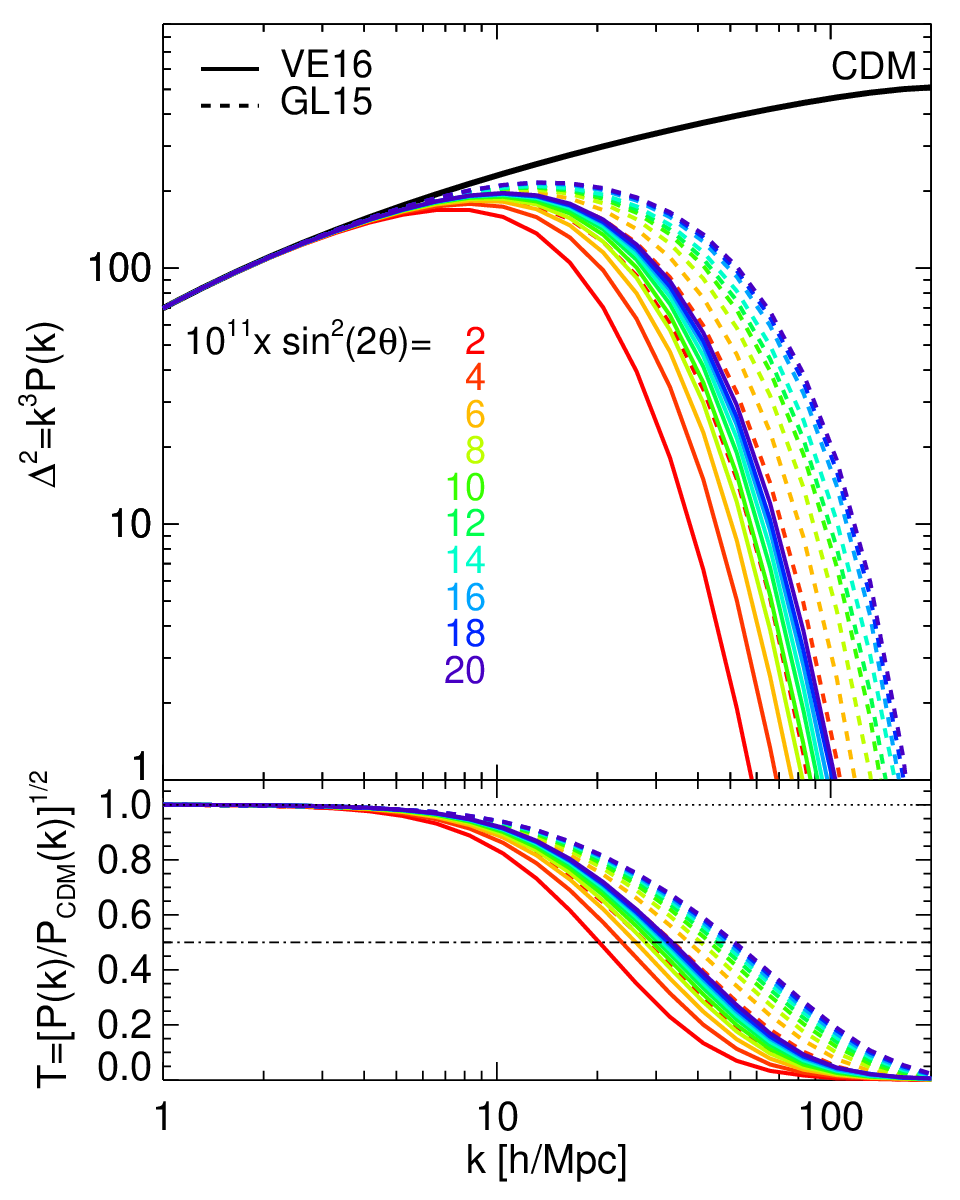
Both codes return the familiar pattern in which the matter power spectrum exhibits a cutoff, and the wavenumber of the cutoff increases with 22 2 Still larger values of would exhibit a turnaround in behaviour, where the cutoff shifts back to smaller wavenumbers as discussed in the previous section. However, these are outside the expected 3.55 keV line constraints and therefore are not considered here.. Where the two codes differ is in the location of the cutoff at fixed : the 56 turnovers are at consistently larger than for 128. This behaviour is more clearly apparent in the ratio with respect to CDM as shown in the bottom panel of Figure 2. It is apparent from this panel that the half mode wavenumber is marginally larger for 56 than it is for 128, thus the value of will be smaller for the former.
The existence of a cutoff at scales corresponding to dwarf galaxies means that are classed as warm dark matter (Bond & Szalay 1983; Bardeen et al. 1986; Bode et al. 2001, WDM; ). Given the desire to have constraints on dark matter cutoffs that are not dependent on any single particle physics candidate, it is common to generate constraints for the thermal relic toy model discussed above. In practice, this is typically achieved through the fit to thermal relic spectra computed in Viel et al. 2005, which links the thermal relic mass to as outlined in Bose et al. 2016a.33 3 Subsequent work by Vogel & Abazajian 2022 has improved upon this fit; however, in cosmology and astrophysics studies it is the Viel et al. 2005 fit that has been used to compute generic WDM limits and therefore we retain their equations in our work.. The Viel et al. 2005 relation in principle does not need to have the same shape as the spectra. Therefore, for each of our curves we compute the half-mode mass and then in turn compute the Viel et al. 2005 power spectrum that has the same . We compute the ratio of each power spectrum to its same- thermal relic counterpart and present the results in Fig. 3. We divide the wavenumber by each models’ half-mode wavenumber, therefore the value of the ratio at equals 1 by construction.

The shallow cutoffs associated with both models significantly reduce the power with respect to the thermal relic approximation for and exhibit more power than the thermal relic at larger wavenumbers. The difference between and the approximation is strongly dependent on , with stronger deviations for larger values of . The 56 model power is suppressed by 20 per cent compared to the thermal relic equivalent compared to 12 per cent for the same code with . The difference is smaller for 128, at 10 per cent for and smaller suppressions for lower values. We therefore expect that the Viel et al. 2005 thermal relic approximation overestimates the power associated with models, especially for the 56 momentum computations.
3.2 Parameter values: lepton asymmetry and the half-mode mass
We have demonstrated that the momentum distribution computation algorithm and parameter choices have a significant impact on the position of the cutoff for fixed and , and will therefore have an impact on . We also stated in Section 2 that the value of required to obtain the correct abundance will also differ substantially. We illustrate the scale of these differences explicitly by computing and as a function of for both codes, and then presenting the results in Fig. 4. We also include the results of previously unpublished computations for the keV using the machinery behind Lovell et al. 2016 and subsequent papers that build on that paper, which itself used an earlier version of the 56 code. We include these results to facilitate comparisons to earlier work; understanding the origins of these differences is beyond the scope of this paper.


The values of differ significantly between the three computational implementations. All three follow the familiar track wherein smaller mixing angles require larger lepton asymmetries to obtain the correct abundance, but the amplitudes of the relations differ considerably. 128 prefers at down to at , whereas the chosen implementation of 56 prefers to over the same range. We stress that this result applies to one specific implementation of 56: alternative choices for the initial asymmetries of separate lepton species can generate overall asymmetries at that are as high as or as low as , as discussed in 56 table 1. This lower value is somewhat closer to the Lovell et al. 2016 implementation, which otherwise requires values much lower than either 128 or our adopted 56 implementation. Therefore, there remains work to be done to estimate the initial lepton asymmetry precisely and accurately.
While the value of is inaccessible to current experiments, is regularly subject to constraints. Both momentum codes return the familiar anticorrelation between and , such that attempts to evade X-ray constraints on lead to stronger structure formation constraints on and vice versa. The amplitude of the relations is significantly different, with the smaller scale power spectrum cutoffs of 56 discussed in 2 leading to smaller by a factor of - than for 128 at fixed . The Lovell et al. 2016 implementation generates a somewhat steeper relation, with some 50 per cent larger than 56 at but approaches the 56 values towards higher . Finally, we generate fits to both implementations of the form
| (4) |
4 Comparison to observations
In this section we assess the current status of X-ray detections and constraints on , and of structure formation constraints on . We then compare some of these constraints to our fits for 128 and 56.
4.1 X-ray detections and constraints
The first reported detections of an X-ray line at 3.55 keV consistent with dark matter decay were made by Bulbul et al. 2014 in clusters of galaxies with the XMM-Newton (‘XMM’) observatory and Boyarsky et al. 2014 in the M31 galaxy and the Perseus galaxy cluster, also with XMM. The values of were estimated as ( errors) for the cluster stack and for M31 on flux statistical uncertainties alone; including M31 mass uncertainties gives . The detection in the centre of Perseus was anomalously high compared to the other results and subsequently ruled out by Aharonian et al. 2017. Further detections have been reported in the MW Galactic bulge at from the Galactic Centre with Chandra (Hofmann & Wegg 2019, ,) and the MW halo contribution to the COSMOS Legacy and Extended Chandra Deep Field South survey fields, also with Chandra (Cappelluti et al. 2018, ,). Other studies have reported constraints that are in strong tension with the claimed detections, including in alternative studies of the Galactic Centre (Jeltema & Profumo 2015), the broader MW halo (Dessert et al. 2020b, see also Boyarsky et al. 2020; Abazajian 2020; Dessert et al. 2020a) and still further studies allow for only a small region of the parameter space of interest to remain (Sicilian et al. 2022; Roach et al. 2023). A stack of galaxies returned strong constraints (Anderson et al. 2015), which motivated exotic dark matter models in which the line was only generated in clusters (Conlon & Powell 2015). Arguably the most promising target for a detection is the Draco dwarf spheroidal galaxy (Lovell et al. 2015), yet 1.4 Ms observation with XMM was insufficient to obtain a detection, and two different groups returned different results (Jeltema & Profumo 2016; Ruchayskiy et al. 2016).
Much of the above uncertainty reflects different approaches to modelling the astrophysical background. An alternative source for the line is charge exchange, in which electrons are accreted from the neutral medium onto sulphur atoms and then generate 3.55 keV photons through the subsequent cascade of atomic transitions (Gu et al. 2015; Shah et al. 2016), resulting in an astrophysical line. One key discriminator between a dark matter decay line and an astrophysical line is its velocity dispersion. Astrophysical line velocity dispersions are typically , while Lovell et al. 2019b showed that for nearby clusters the velocity dispersion is instead - depending on the cluster. This measurement requires a high resolution X-ray calorimeter not available to the galaxy cluster studies discussed above. It had been hoped that the Hitomi mission would make the required measurement with its state-of-the-art calorimeter, but the mission was lost after a month and the data obtained prior to the failure were not sufficient to detect the line feature (Aharonian et al. 2017). The next opportunity to test the line velocity dispersion will come with the XRISM mission (Terada et al. 2021).
4.2 Structure formation and cosmological constraints
Cosmological and structure formation constraints have been derived in a wide variety of astronomical observables, including the CMB, BBN, the Lyman- forest, gravitational lensing, stellar streams around the MW, reionization studies and MW satellite counts. We summarize the status of each of these fields below. Many of the cosmological constraints are defined for a generic thermal relic WDM model. They typically assume the WDM thermal relic power spectrum using the parameter; recall that this reflects an approximation to the power spectrum and is not the same as the mass. Throughout this section we will refer to constraints on the WDM model rather than , except where noted otherwise.
Part of the challenge in setting limits through these studies is the difficulty in selecting a lower effective prior on the parameters. of viable true thermal relic models is MeV (Depta et al. 2019; Sabti et al. 2020) and is CDM, whereas the effective for a classical axion model may well be much larger than this, and all at much larger values than the 1-10 keV expected for WDM. One approach is to instead constraint , which for CDM . This option evades the infinity but still creates a problem in logarithmic limits, a problem that is shared by . Most studies typically quote a limit on each parameter at 95 per cent confidence level (95 C. L.), based on the probability distribution of a posterior likelihood. Some studies also quote the highest (lowest ) for which the likelihood is 5 per cent of the maximum likelihood amplitude (5 M. L.). The latter measure is more conservative and evades the issue of how to determine the lower end of the prior. Therefore, we will set a preference to use this option in what follows, including inferring this result from paper results where possible.
4.2.1 Early Universe constraints
If and are sufficiently long-lived, with lifetime s, they will interfere significantly with BBN, it is thus possible to show that (Serpico & Raffelt 2005). Moreover, it is conceivable that if a sufficient fraction of the sterile neutrinos remain relativistic to late times, they may add a contribution to the number of relativistic degrees of freedom, . Our class calculations return for all 128 and 56 models, which is significantly smaller than the figure (95 C. L.) of Planck Collaboration et al. 2020. We present these results in more detail in Appendix A.
4.2.2 The Lyman- forest
Lyman- constraints take advantage of the suppression of structure at redshifts . They examine fine hydrogen absorption features in the spectra of high redshift quasars – the Lyman- forest – to infer the amount of structure present in the gas, and convolve these results with expectations for the properties of gas physics to obtain the underlying dark matter distribution. Progressively stronger constraints have been reported, from keV (Viel et al. 2005) at 95 C. L. through to keV (95 C. L.) (Iršič et al. 2017) (see also Murgia et al. 2017); we infer keV 5 M. L. for these data. Arguably the primary source of uncertainty is the thermal history, which may either mimic or obscure a dark matter power spectrum cutoff (Garzilli et al. 2017). A recent analysis by Villasenor et al. 2023 used new data sets and a different approach to the thermal history. They set a limit of keV (95 C. L.; we infer keV for 5 M. L.) and reported a weak preference for keV over the CDM model.
4.2.3 Gravitation lensing
While the Lyman forest studies use a background light source to detect a power spectrum cutoff through absorption, gravitational lensing experiments instead infer dark matter properties from how the background source is either distorted or magnified. The background light is lensed by a foreground dark matter halo – typically an isolated elliptical galaxy – and the degree of dark matter substructure is determined by the degree to which the lensing signal deviates from that expected for a smooth lens. This method has the potential to detect dark matter haloes down to , where haloes are expected to contain no gas and thus remain dark. The two subbranches of lensing relevant for linear matter power spectrum studies are flux anomalies, in which the background source is a multiply imaged quasar, and gravitational imaging, which instead analyses lensed images of extended galaxies.
The gravitational lensing method has successfully detected several massive ( ) haloes (Vegetti et al. 2010; Hezaveh et al. 2016), but not to a degree sufficient to compute strong constraints on the WDM model (Vegetti et al. 2018; Ritondale et al. 2019), and Euclid and the Vera C. Rubin Observatory (VCRO) will not have enough angular resolution to improve the constraints (O’Riordan et al. 2023). It is expected that high resolution imaging from the European Extremely Large Telescope (E-ELT) or very large baseline interferometry coupled to the square kilometre-array (McKean et al. 2015; Powell et al. 2023) will be required to obtain sufficient statistics. Recent work in the flux anomalies side has claimed stronger constraints: Gilman et al. 2020 reports keV 95 C. L. ( keV at 5 M. L., see Zelko et al. 2022 for an application of this result to sterile neutrino models), and Hsueh et al. 2020 find keV 95 C. L.,44 4 We do not infer a 5 M. L. limit for this result because the joint posterior amplitude is higher than 5 per cent of its maximum at all quoted masses. although the latter also reports the role of systematic uncertainties that require further study to refine this constraint. The Euclid mission may detect enough flux anomalies systems to discern whether the flux anomaly distribution is better described by CDM or WDM (Harvey et al. 2020).
4.2.4 Stellar stream gaps
An alternative method for detecting dark subhaloes is to search for their impact on gaps in stellar streams up to kpc from the MW centre. Stellar streams are generated through the tidal stripping of globular clusters and satellite galaxies by the MW, and are expected to be very smooth in their light profile. The detection of kinks or gaps in a stream is then evidence for a past interaction with a perturber, including dark matter subhaloes. One reported detection of such a perturbation was made by Bonaca et al. 2019. Banik et al. 2021 reported keV (95 C. L.) based on expectations for the MW subhalo mass function in WDM. However, the subhalo mass function in the central kpc differs less from CDM than is the case for the halo as a whole (Lovell et al. 2021); taking this factor into account weakens the constraint to keV (95 C. L.).
4.2.5 High redshift constraints
The previous three types of studies looked for gravitationally induced distortions on observables. One further approach is to detect light from dwarf galaxies, whose number density is suppressed in WDM models. One such source of light is low mass galaxies in the early Universe, the presence or absence of which impacts the rate of reionization and thus determines when the Universe becomes transparent to visible light/mildly opaque to CMB photons. Various studies have considered the possibility of detecting these galaxies directly or instead comparing to reionization constraints. This possibility has been considered using a variety of simulation- and semi-analytic model-based approaches (Schultz et al. 2014; Bose et al. 2016b; Menci et al. 2016; Rudakovskyi & Iakubovskyi 2016; Lovell et al. 2019a; Rudakovskyi et al. 2021; Kurmus et al. 2022; Maio & Viel 2023). These papers reveal that the impact of the cutoff is highly degenerate with gas physics processes such as the escape fraction of photons, and are therefore results in constraints weaker than those of the other observables listed above. The reported limits include keV (Menci et al. 2016, 95 C. L., ), and keV (Rudakovskyi & Iakubovskyi 2016; Maio & Viel 2023).
4.2.6 MW satellite counts
The final method that we will consider here for generating constraints is the detection of MW satellite galaxies. The MW satellites are the faintest observable galaxies, and therefore probe the edge of reionization as well as the subhalo mass function at . Constraints rely on estimating the true number of MW satellites: approximately 50 are known (Bechtol et al. 2015; Drlica-Wagner et al. 2015; Torrealba et al. 2016; Koposov et al. 2018, e.g.) and the number of undetected satellites are inferred from completeness limits due to depth and sky coverage. Very conservative limits can be obtained for values of keV where the number of satellites generated is even smaller than the number of known MW satellites (Lovell et al. 2014) and marginally less conservative limits return keV (Polisensky & Ricotti 2011).
Stronger limits require an understanding of the sky coverage selection function discussed above as well as physical processes such as the evacuation of gas from low mass haloes during reionization, the disruption of satellites by the MW disc, uncertainties in the MW halo mass, stochastic variations in halo assembly and the role of the Large Magellanic Cloud (LMC). Different assumptions in these areas can lead to dramatic differences in the number of predicted satellites: Cherry & Horiuchi 2017 estimated satellites, the compilation by Kim et al. 2018 reports 120-150 satellites, the analysis by Newton et al. 2018 expects satellites, and Nadler et al. 2020 instead predicts of order 220. These results are key inputs for further studies of both WDM generally (Enzi et al. 2021; Nadler et al. 2021; Newton et al. 2021) and (Dekker et al. 2022; Zelko et al. 2022), and we discuss these at the end of this subsection.
4.2.7 MW satellite structure
We end this review on the interplay between the WDM model and astrophysical observations with a discussion of the structure of MW satellites. The density of haloes with masses around the cutoff scale is suppressed in WDM relative to CDM (Colín et al. 2000; Lovell et al. 2012), and the degree of suppression is sufficient to explain a claimed discrepancy in the masses of subhaloes in CDM simulations versus observed satellites known as the ‘Too Big To Fail’ problem (Boylan-Kolchin et al. 2011; Boylan-Kolchin et al. 2012; Lovell et al. 2012; Horiuchi et al. 2016; Lovell et al. 2017a; Lovell et al. 2017b; Bozek et al. 2019; Lovell & Zavala 2023). In principle, the density profiles of these satellites are the single most informative source for discriminating between different dark matter models: from high concentration cusps in CDM (Navarro et al. 1996b; Navarro et al. 1997) to lower concentration cusps in WDM (Lovell et al. 2014); from self-interacting dark matter (SIDM) cores (Vogelsberger et al. 2012) to the very steep gravothermally collapsed cusps in extreme SIDM models (Zavala et al. 2019) and even the solitons of fuzzy dark matter (Nori et al. 2023). However, in the faintest systems it is very challenging to obtain enough stars to compute a density profile, and in brighter galaxies supernova feedback may play a confounding role (Navarro et al. 1996a; Pontzen & Governato 2012). Therefore, we do not attempt to provide WDM parameter constraints using satellite densities but highlight the importance of this observable for future dark matter studies.
4.2.8 Combined constraints
Several of the studies discussed above have reported combined constraints that convolve posterior distributions from a number of different observations. These include Enzi et al. 2021, Nadler et al. 2021 and Zelko et al. 2022. In all cases the strongest limits are provided by the satellite count component: therefore, as stated above for the two studies that constrain the Viel et al. 2005 thermal relic model, (5 M. L.) for Enzi et al. 2021 and (5 M. L.) for Nadler et al. 2021. As we will demonstrate below, the difference between these results brackets the allowed range for 3.55 keV line-compliant .
4.3 Comparison to sterile neutrino parameter relations
In the previous two subsections we have presented limits from observations on /WDM parameters. X-ray non-detections enforce lower values of , and WDM structure formation arguments decrease the allowed . Given that and are anticorrelated, it is therefore possible to compare these in tension to estimate the optimal parameters, if any, that are permitted by the observations or even preferred by reported detections.
In Fig. 5, we compare some of the X-ray and structure formation constraints listed above to the equation 4 fits to 128 and 56. Upper limits on are shown as horizontal lines with down-facing arrows, and upper limits on from X-ray studies are shown vertical lines with left-facing arrows; X-ray detections are shown as error bars. Each constraint only applies to either or , and therefore its line applies across all of the presented parameter space; we draw short lines for the sake of clarity. We include four reported detections that span a range of targets: the M31 detection of Boyarsky et al. 2014, the galaxy cluster stack of Bulbul et al. 2014, the Galactic bulge detection by Hofmann & Wegg 2019, and the outer MW halo detection of Cappelluti et al. 2018 when adopting the high-mass MW halo parameters. We represent non-detections with two of the most stringent available: the galaxy stack of Anderson et al. 2015 and the MW halo work of Sicilian et al. 2022 (Dessert et al. 2020b; Boyarsky et al. 2020; Dessert et al. 2020a, for further analysis of the MW halo see). Finally, for constraints we include five studies that quote, or from which we can obtain, 5 M. L. limits: two Lyman- results (Iršič et al. 2017; Villasenor et al. 2023), one gravitational lensing study (Gilman et al. 2020) and two combined-observation analyses that are in practice dominated by MW satellite counts (Enzi et al. 2021; Nadler et al. 2021)55 5 Strong constraints have also been presented by Kim et al. 2018 ( keV, MW satellite counts) and Hsueh et al. 2020 (, 95 C. L., gravitational lensing); it is not possible to obtain 5 M. L. limits from these studies..

In both the X-ray observations and the structure formation analyses, there is a wide variety of inconsistent constraints, some of which are in strong tension with both model predictions. The satellite counts in Nadler et al. 2021 are incompatible with any part of the suggested parameter space, with whereas the alternative analysis by Enzi et al. 2021 is consistent with all models but for the 128 model with . These studies are strongly dependent on the modelling of the LMC satellite contribution, the disruption of satellites by the disc, and the mass of MW halo, each of which leads to the differences in these results. There is similar disagreement within the Lyman- bounds, where the Iršič et al. 2017 limit rules out all models while Villasenor et al. 2023 is consistent with 56 for . The Gilman et al. 2020 limit is consistent with 56 for and rules out all of the 128 options.
The X-ray results are similarly inconsistent. We quote two non-detection studies, Sicilian et al. 2022 and Anderson et al. 2015, that are strongly constraining. The Sicilian et al. 2022 result permits , which is consistent with the Hofmann & Wegg 2019 detection but in some tension with the other. It would also require for 56. The Anderson et al. 2015 analysis is instead inconsistent with all of the allowed range. As for the reported detections, there is no one value of that is consistent with the ranges of all four. Adopting the value of would represent a median between the four observations; if one instead posited that there is an undetected systematic uncertainty in the MW halo-derived results – both for the Hofmann & Wegg 2019 detection and for the limits by Dessert et al. 2020b; Dessert et al. 2020a and Sicilian et al. 2022 – that underestimates then one can make a case for .
The question then becomes how to process these data into a coherent picture. The simplest approach is to take the most stringent constraints at face value, in which case both of the implementations discussed here are ruled out through a combination of the Anderson et al. 2015 galaxy stack and the Nadler et al. 2021 satellite counts. One then has to consider either that further iterations of the momentum distribution calculation will return values of that are lower by at least a factor of 20 compared to 56, in order to obtain at , or that resonantly produced keV s as a whole are not viable and should be discarded as a dark matter candidate. If one were to be more optimistic, one could attempt to determine a provisional value of , first by comparing the detections and then factoring in those X-ray and structure formation constraints that do result in a coherent – pair. The rough mid-point of the reported detections would return ; relaxing the contribution of the MW halo could instead lead to and then using 56. This choice still gives the Sicilian et al. 2022 constraint and higher than the Iršič et al. 2017 constraint. Given that privileging one constraint will lead to greater tension with the other, we will argue that the single best value of for future study is , with – and by extension keV – as calculated with 56. This value is also well within the preferred region for determined by Villasenor et al. 2023. We focus on this model for future study and for a comprehensive evaluation together with the strongest reported constraints.
5 Conclusions
The resonantly produced sterile neutrino () constitutes a compelling dark matter candidate for several reasons. It is part of a larger theory that may also explain neutrino oscillations and baryogenesis (Dodelson & Widrow 1994; Dolgov & Hansen 2002; Asaka & Shaposhnikov 2005; Laine & Shaposhnikov 2008; Boyarsky et al. 2009a), as well as adding right-handed neutrinos to the standard model. It is also accessible to astronomical experiments, through its decay into X-rays for large mixing angles (Pal & Wolfenstein 1982; Abazajian et al. 2001a; Abazajian et al. 2001b) and its erasure of structure at small mixing angles (Dodelson & Widrow 1994; Shi & Fuller 1999; Laine & Shaposhnikov 2008; Lovell et al. 2016). Detections of an X-ray signal claimed to be compatible with the decay of a with mass keV and mixing angle add extra motivation. In this paper we revisit the physics behind production and its role in neutrino oscillations and baryons, present how different computational methods reach different conclusions for the linear matter power spectrum, and compare the results to observational constraints.
The MSM proposes the addition of three sterile neutrinos to the standard model. If two of these sterile neutrinos have masses at the GeV scale ( and ) and is at the keV scale, and can facilitate baryogenesis and neutrino oscillations while is a dark matter candidate. The same process that leads and to generate the baryon asymmetry of the Universe may also lead to a lepton asymmetry at later times, which then enables the resonant production of . This resonant production leads to a momentum distribution that is skewed towards lower momenta than is the case for non-resonant production. The result is that the model behaves as WDM.
Two different publicly available codes – published in 128 and 56 – compute the momentum distributions for , determining the correct value of the lepton asymmetry, , to obtain the required dark matter abundance. We echo the result of 128 in demonstrating that their code generates a warmer matter power spectrum than does 56 (Fig. 2). Sterile neutrino models are often approximated by thermal relic power spectra: we show that the thermal relic model overestimates the power in sterile neutrino models for by up to 20 per cent, especially for larger (Fig. 3). The value of for 128 and the chosen implementation of 56 varies by 26 per cent (Fig. 4), but further implementations will differ by a factor of 10 (56). We also compute the half-mode mass as a function of , and show this variable can vary by up to a factor of 5 between the two implementations.
We discuss the current status of constraints of dark matter decay from X-rays and the limits on the WDM cutoff scale from structure formation measurements. We present four detections of the 3.55 keV line centred on and several non-detections that prefer . We also discuss structure formation constraints on from the Lyman- forest, gravitational lensing, stream gaps, and MW satellite counts. We show that the satellite counts currently offer the strongest constraints, and competing analyses offer limits that bracket the range: at 5 M. L. for Enzi et al. 2021 and at 5 M. L. for Nadler et al. 2021 (Fig. 5). If we adopt the most stringent published constraints, then dark matter is ruled out; if we instead take an optimistic approach then the combination of and constraints suggests the average detection of is most likely.
The clearest test of this result in the near future is the launch of the XRISM mission. This facility features a high resolution calorimeter that will measure the widths of X-ray lines, which in clusters of galaxies are characteristically larger for dark matter decay ( ) than for astrophysical lines ( ). The performance verification (PV) phase for XRISM will include the following guaranteed observation time: 280 ks for the Perseus cluster – comparable to the 230 ks obtained by Hitomi before that mission was lost – plus 500 ks of the Virgo cluster, 150 ks of the Centaurus cluster and 200 ks of the Coma cluster, with an additional 200 ks for Perseus and 100 ks for Coma if conditions allow (https://heasarc.gsfc.nasa.gov/docs/xrism/timelines/pvtargets.html).
The Perseus, Virgo, and Centaurus decay line parameters were estimated for the XRISM field of view in Lovell et al. 2019b, with on-centre line-of-sight velocity dispersions , and respectively. The Coma cluster mass and distance parameters are approximately the same as Perseus and therefore this cluster should also have . Lovell et al. 2019b also estimated that the expected flux from Virgo should be twice that of Perseus, thus when combined with the PV time allocations suggests that Virgo may present the first opportunity to detect the line, prior to the consideration of other observational effects. Bulbul et al. 2014 estimated that a Perseus line of – the velocity dispersion of the Perseus member galaxies rather than the dark matter – could be detected with 1 Ms of exposure, which is the maximum Perseus PV allocation but to first order returns the same number of photons as the 500 ks Virgo allocation, given that the expected Virgo flux is twice that of Perseus and also that the line width in Virgo is half that of the Bulbul et al. 2014-Perseus estimate. The tentative detection of a line in Virgo would then motivate dedicated, post-PV campaigns to measure the line width in other nearby clusters and ascertain whether or not its properties strictly adhere to the dark matter content.
In the event that such a detection is made, two questions will arise: (i) whether the line is indeed dark matter decay, and (ii) whether this candidate is dark matter. First, the following steps will need to be taken to ascertain that the line is dark matter decay:
- •
Obtain careful estimates of the astrophysical background signal in galaxies and galaxy clusters, empirically from observations and also from mock observations of simulations.
- •
Perform observations of targets where the amount of hot gas is minimized, such as the Bullet cluster (Boyarsky et al. 2008) and the Draco dSph (Lovell et al. 2015).
- •
Develop sophisticated models of the MW halo mass distribution, including adiabatic contraction, to compare to blank sky X-ray observations.
Second, we set out the issues to be addressed in ascertaining whether this decaying dark matter is rather than a still more exotic candidate:
- •
Refine the computations of early Universe physics to ascertain as accurately as possible the initial lepton asymmetry and the momentum distribution.
- •
Identify whether differences between the full matter power spectra calculations and the thermal relic approximation are significant for structure formation constraints.
- •
Ascertain the source of the current incompatibility in MW satellite counts, and then resolve the discrepancy, including through new observations by the upcoming VCRO-LSST facility (Ivezić et al. 2019).
- •
Perform high-resolution gravitational imaging studies with the E-ELT to measure the halo mass function (Vegetti et al. 2018).
- •
Continue to develop models of galaxy formation that accurately follow processes as diverse as star formation, supernova feedback, magnetic fields, and stripping by host galaxies in order to predict halo density profiles and luminosity fractions, particularly in dSphs (Gutcke et al. 2022).
- •
Pursue efforts to detect other candidates, such as low-reheating temperature models where the signal is explained by a particle that is only a small fraction of the dark matter (Abazajian 2017) and could be experimentally detected by the proposed HUNTER experiment (Martoff et al. 2021).
One final consideration is the contribution from particle physics experiments. Generating measurable amount of in an experiment is a formidable challenge, where even the anticipated upgrades to the KATRIN experiment are limited to probing (Aker et al. 2022), some two orders of magnitude higher than the lowest 3.55 keV line-compatible models. Other experiments are instead searching for and . The DUNE experiment will probe neutrino physics to ascertain the neutrino mass hierarchy and measure the charge-parity-violating phase, and has some potential to constrain the parameter space of and (DUNE Collaboration et al. 2015; DUNE Collaboration et al. 2020); it will come online in the second half of this decade. Two proposed CERN experiments, SHiP (Ahdida et al. 2019) and MATHUSLA (Curtin et al. 2019), would probe rare events in which and are produced and then decay into products that are subsequently detected. The combination of experiment, X-ray observations, and structure formation constraints will then have played a key role in identifying whether is indeed the dark matter.
Acknowledgements
MRL would like to thank Jesús Zavala, Tamar Meshveliani, Esra Bulbul, Michael Boylan-Kolchin, Francis-Yan Cyr-Racine, Simona Vegetti and the anonymous referee for useful comments.
Data Availability
The original codes for 128 and 56 are available at https://github.com/ntveem/sterile-dm and http://www.laine.itp.unibe.ch/dmpheno/ respectively.
References
- Abazajian (2014) Abazajian K. N., 2014, Physical Review Letters, 112, 161303
- Abazajian (2017) Abazajian K. N., 2017, Phys. Rep., 711, 1
- Abazajian (2020) Abazajian K. N., 2020, arXiv e-prints, p. arXiv:2004.06170
- Abazajian & Kusenko (2019) Abazajian K. N., Kusenko A., 2019, Phys. Rev. D, 100, 103513
- Abazajian et al. (2001a) Abazajian K., Fuller G. M., Patel M., 2001a, Phys. Rev. D, 64, 023501
- Abazajian et al. (2001b) Abazajian K., Fuller G. M., Tucker W. H., 2001b, ApJ, 562, 593
- Abratenko et al. (2023) Abratenko P., et al., 2023, Phys. Rev. Lett., 130, 011801
- Adhikari et al. (2017) Adhikari R., et al., 2017, J. Cosmology Astropart. Phys., 2017, 025
- Agafonova et al. (2023) Agafonova N., et al., 2023, Progress of Theoretical and Experimental Physics, 2023, 033C01
- Aharonian et al. (2017) Aharonian F. A., et al., 2017, ApJ, 837, L15
- Ahdida et al. (2019) Ahdida C., et al., 2019, Journal of High Energy Physics, 2019, 77
- Aker et al. (2022) Aker M., et al., 2022, Journal of Physics G Nuclear Physics, 49, 100501
- An et al. (2022) An R., Gluscevic V., Calabrese E., Hill J. C., 2022, J. Cosmology Astropart. Phys., 2022, 002
- An et al. (2023) An R., Gluscevic V., Nadler E. O., Zhang Y., 2023, arXiv e-prints, p. arXiv:2301.08299
- Anderson et al. (2015) Anderson M. E., Churazov E., Bregman J. N., 2015, MNRAS, 452, 3905
- Asaka & Shaposhnikov (2005) Asaka T., Shaposhnikov M., 2005, Physics Letters B, 620, 17
- Athanassopoulos et al. (1996) Athanassopoulos C., et al., 1996, Phys. Rev. Lett., 77, 3082
- Banik et al. (2021) Banik N., Bovy J., Bertone G., Erkal D., de Boer T. J. L., 2021, J. Cosmology Astropart. Phys., 2021, 043
- Bardeen et al. (1986) Bardeen J. M., Bond J. R., Kaiser N., Szalay A. S., 1986, ApJ, 304, 15
- Barger et al. (1995) Barger V., Phillips R. J. N., Sarkar S., 1995, Physics Letters B, 352, 365
- Bechtol et al. (2015) Bechtol K., et al., 2015, ApJ, 807, 50
- Bode et al. (2001) Bode P., Ostriker J. P., Turok N., 2001, ApJ, 556, 93
- Bonaca et al. (2019) Bonaca A., Hogg D. W., Price-Whelan A. M., Conroy C., 2019, ApJ, 880, 38
- Bond & Szalay (1983) Bond J. R., Szalay A. S., 1983, ApJ, 274, 443
- Bose et al. (2016a) Bose S., Hellwing W. A., Frenk C. S., Jenkins A., Lovell M. R., Helly J. C., Li B., 2016a, MNRAS, 455, 318
- Bose et al. (2016b) Bose S., Frenk C. S., Hou J., Lacey C. G., Lovell M. R., 2016b, MNRAS, 463, 3848
- Boyarsky et al. (2008) Boyarsky A., Ruchayskiy O., Markevitch M., 2008, ApJ, 673, 752
- Boyarsky et al. (2009a) Boyarsky A., Ruchayskiy O., Shaposhnikov M., 2009a, Annual Review of Nuclear and Particle Science, 59, 191
- Boyarsky et al. (2009b) Boyarsky A., Lesgourgues J., Ruchayskiy O., Viel M., 2009b, Physical Review Letters, 102, 201304
- Boyarsky et al. (2014) Boyarsky A., Ruchayskiy O., Iakubovskyi D., Franse J., 2014, Physical Review Letters, 113, 251301
- Boyarsky et al. (2020) Boyarsky A., Malyshev D., Ruchayskiy O., Savchenko D., 2020, arXiv e-prints, p. arXiv:2004.06601
- Boylan-Kolchin et al. (2011) Boylan-Kolchin M., Bullock J. S., Kaplinghat M., 2011, MNRAS, 415, L40
- Boylan-Kolchin et al. (2012) Boylan-Kolchin M., Bullock J. S., Kaplinghat M., 2012, MNRAS, 422, 1203
- Bozek et al. (2016) Bozek B., Boylan-Kolchin M., Horiuchi S., Garrison-Kimmel S., Abazajian K., Bullock J. S., 2016, MNRAS, 459, 1489
- Bozek et al. (2019) Bozek B., et al., 2019, MNRAS, 483, 4086
- Bulbul et al. (2014) Bulbul E., Markevitch M., Foster A., Smith R. K., Loewenstein M., Randall S. W., 2014, ApJ, 789, 13
- Canetti et al. (2013a) Canetti L., Drewes M., Frossard T., Shaposhnikov M., 2013a, Phys. Rev. D, 87, 093006
- Canetti et al. (2013b) Canetti L., Drewes M., Shaposhnikov M., 2013b, Phys. Rev. Lett., 110, 061801
- Cappelluti et al. (2018) Cappelluti N., et al., 2018, ApJ, 854, 179
- Cherry & Horiuchi (2017) Cherry J. F., Horiuchi S., 2017, Phys. Rev. D, 95, 083015
- Colín et al. (2000) Colín P., Avila-Reese V., Valenzuela O., 2000, ApJ, 542, 622
- Conlon & Powell (2015) Conlon J. P., Powell A. J., 2015, J. Cosmology Astropart. Phys., 2015, 019
- Curtin et al. (2019) Curtin D., et al., 2019, Reports on Progress in Physics, 82, 116201
- DUNE Collaboration et al. (2015) DUNE Collaboration et al., 2015, arXiv e-prints, p. arXiv:1512.06148
- DUNE Collaboration et al. (2020) DUNE Collaboration et al., 2020, arXiv e-prints, p. arXiv:2008.12769
- Dekker et al. (2022) Dekker A., Ando S., Correa C. A., Ng K. C. Y., 2022, Phys. Rev. D, 106, 123026
- Depta et al. (2019) Depta P. F., Hufnagel M., Schmidt-Hoberg K., Wild S., 2019, J. Cosmology Astropart. Phys., 2019, 029
- Dessert et al. (2020a) Dessert C., Rodd N. L., Safdi B. R., 2020a, Physics of the Dark Universe, 30, 100656
- Dessert et al. (2020b) Dessert C., Rodd N. L., Safdi B. R., 2020b, Science, 367, 1465
- Dodelson & Widrow (1994) Dodelson S., Widrow L. M., 1994, Physical Review Letters, 72, 17
- Dolgov & Hansen (2002) Dolgov A. D., Hansen S. H., 2002, Astroparticle Physics, 16, 339
- Drlica-Wagner et al. (2015) Drlica-Wagner A., et al., 2015, ApJ, 813, 109
- Enzi et al. (2021) Enzi W., et al., 2021, MNRAS, 506, 5848
- Garzilli et al. (2017) Garzilli A., Boyarsky A., Ruchayskiy O., 2017, Physics Letters B, 773, 258
- Gaskins (2016) Gaskins J. M., 2016, Contemporary Physics, 57, 496
- Ghiglieri & Laine (2015) Ghiglieri J., Laine M., 2015, Journal of High Energy Physics, 2015, 171
- Gilman et al. (2020) Gilman D., Birrer S., Nierenberg A., Treu T., Du X., Benson A., 2020, MNRAS, 491, 6077
- Gu et al. (2015) Gu L., Kaastra J., Raassen A. J. J., Mullen P. D., Cumbee R. S., Lyons D., Stancil P. C., 2015, A&A, 584, L11
- Gutcke et al. (2022) Gutcke T. A., Pfrommer C., Bryan G. L., Pakmor R., Springel V., Naab T., 2022, ApJ, 941, 120
- Harvey et al. (2020) Harvey D., Valkenburg W., Tamone A., Boyarsky A., Courbin F., Lovell M., 2020, MNRAS, 491, 4247
- Hezaveh et al. (2016) Hezaveh Y. D., et al., 2016, ApJ, 823, 37
- Hofmann & Wegg (2019) Hofmann F., Wegg C., 2019, A&A, 625, L7
- Horiuchi et al. (2016) Horiuchi S., Bozek B., Abazajian K. N., Boylan-Kolchin M., Bullock J. S., Garrison-Kimmel S., Onorbe J., 2016, MNRAS, 456, 4346
- Hsueh et al. (2020) Hsueh J. W., Enzi W., Vegetti S., Auger M. W., Fassnacht C. D., Despali G., Koopmans L. V. E., McKean J. P., 2020, MNRAS, 492, 3047
- Humbert et al. (2015) Humbert P., Lindner M., Smirnov J., 2015, Journal of High Energy Physics, 2015, 35
- Ibata et al. (2020) Ibata R., Thomas G., Famaey B., Malhan K., Martin N., Monari G., 2020, ApJ, 891, 161
- Iršič et al. (2017) Iršič V., et al., 2017, Phys. Rev. D, 96, 023522
- Ivezić et al. (2019) Ivezić Ž., et al., 2019, ApJ, 873, 111
- Jeltema & Profumo (2015) Jeltema T., Profumo S., 2015, MNRAS, 450, 2143
- Jeltema & Profumo (2016) Jeltema T., Profumo S., 2016, MNRAS, 458, 3592
- Kim et al. (2018) Kim S. Y., Peter A. H. G., Hargis J. R., 2018, Phys. Rev. Lett., 121, 211302
- Koposov et al. (2018) Koposov S. E., et al., 2018, MNRAS, 479, 5343
- Kurmus et al. (2022) Kurmus A., Bose S., Lovell M., Cyr-Racine F.-Y., Vogelsberger M., Pfrommer C., Zavala J., 2022, MNRAS, 516, 1524
- Kusenko (2006) Kusenko A., 2006, Phys. Rev. Lett., 97, 241301
- Laine & Shaposhnikov (2008) Laine M., Shaposhnikov M., 2008, J. Cosmology Astropart. Phys., 6, 31
- Lesgourgues & Tram (2011) Lesgourgues J., Tram T., 2011, J. Cosmology Astropart. Phys., 2011, 032
- Lewis et al. (2000) Lewis A., Challinor A., Lasenby A., 2000, ApJ, 538, 473
- Lovell & Zavala (2023) Lovell M. R., Zavala J., 2023, MNRAS, 520, 1567
- Lovell et al. (2012) Lovell M. R., et al., 2012, MNRAS, 420, 2318
- Lovell et al. (2014) Lovell M. R., Frenk C. S., Eke V. R., Jenkins A., Gao L., Theuns T., 2014, MNRAS, 439, 300
- Lovell et al. (2015) Lovell M. R., Bertone G., Boyarsky A., Jenkins A., Ruchayskiy O., 2015, MNRAS, 451, 1573
- Lovell et al. (2016) Lovell M. R., et al., 2016, MNRAS, 461, 60
- Lovell et al. (2017a) Lovell M. R., Gonzalez-Perez V., Bose S., Boyarsky A., Cole S., Frenk C. S., Ruchayskiy O., 2017a, MNRAS, 468, 2836
- Lovell et al. (2017b) Lovell M. R., et al., 2017b, MNRAS, 468, 4285
- Lovell et al. (2019a) Lovell M. R., Zavala J., Vogelsberger M., 2019a, MNRAS, 485, 5474
- Lovell et al. (2019b) Lovell M. R., Iakubovskyi D., Barnes D., Bose S., Frenk C. S., Theuns T., Hellwing W. A., 2019b, ApJ, 875, L24
- Lovell et al. (2021) Lovell M. R., Cautun M., Frenk C. S., Hellwing W. A., Newton O., 2021, MNRAS, 507, 4826
- Maio & Viel (2023) Maio U., Viel M., 2023, A&A, 672, A71
- Martoff et al. (2021) Martoff C. J., et al., 2021, Quantum Science and Technology, 6, 024008
- McKean et al. (2015) McKean J., et al., 2015, in Advancing Astrophysics with the Square Kilometre Array (AASKA14). p. 84 (arXiv:1502.03362), doi:10.22323/1.215.0084
- Menci et al. (2016) Menci N., Grazian A., Castellano M., Sanchez N. G., 2016, ApJ, 825, L1
- Mention et al. (2011) Mention G., Fechner M., Lasserre T., Mueller T. A., Lhuillier D., Cribier M., Letourneau A., 2011, Phys. Rev. D, 83, 073006
- Merle et al. (2016) Merle A., Schneider A., Totzauer M., 2016, J. Cosmology Astropart. Phys., 2016, 003
- Mikheev & Smirnov (1986) Mikheev S. P., Smirnov A. I., 1986, Nuovo Cimento C Geophysics Space Physics C, 9, 17
- Murgia et al. (2017) Murgia R., Merle A., Viel M., Totzauer M., Schneider A., 2017, J. Cosmology Astropart. Phys., 2017, 046
- Nadler et al. (2020) Nadler E. O., et al., 2020, ApJ, 893, 48
- Nadler et al. (2021) Nadler E. O., Birrer S., Gilman D., Wechsler R. H., Du X., Benson A., Nierenberg A. M., Treu T., 2021, ApJ, 917, 7
- Navarro et al. (1996a) Navarro J. F., Eke V. R., Frenk C. S., 1996a, MNRAS, 283, L72
- Navarro et al. (1996b) Navarro J. F., Frenk C. S., White S. D. M., 1996b, ApJ, 462, 563
- Navarro et al. (1997) Navarro J. F., Frenk C. S., White S. D. M., 1997, ApJ, 490, 493
- Newton et al. (2018) Newton O., Cautun M., Jenkins A., Frenk C. S., Helly J. C., 2018, MNRAS, 479, 2853
- Newton et al. (2021) Newton O., et al., 2021, J. Cosmology Astropart. Phys., 2021, 062
- Nori et al. (2023) Nori M., Macciò A. V., Baldi M., 2023, MNRAS, 522, 1451
- O’Riordan et al. (2023) O’Riordan C. M., Despali G., Vegetti S., Lovell M. R., Moliné Á., 2023, MNRAS, 521, 2342
- Pal & Wolfenstein (1982) Pal P. B., Wolfenstein L., 1982, Phys. Rev. D, 25, 766
- Petreczky (2012) Petreczky P., 2012, Journal of Physics G Nuclear Physics, 39, 093002
- Planck Collaboration et al. (2016) Planck Collaboration et al., 2016, A&A, 594, A13
- Planck Collaboration et al. (2020) Planck Collaboration et al., 2020, A&A, 641, A6
- Polisensky & Ricotti (2011) Polisensky E., Ricotti M., 2011, Phys. Rev. D, 83, 043506
- Pontzen & Governato (2012) Pontzen A., Governato F., 2012, MNRAS, 421, 3464
- Powell et al. (2023) Powell D. M., Vegetti S., McKean J. P., White S. D. M., Ferreira E. G. M., May S., Spingola C., 2023, MNRAS, 524, L84
- Ritondale et al. (2019) Ritondale E., Vegetti S., Despali G., Auger M. W., Koopmans L. V. E., McKean J. P., 2019, MNRAS, 485, 2179
- Roach et al. (2023) Roach B. M., et al., 2023, Phys. Rev. D, 107, 023009
- Ruchayskiy et al. (2016) Ruchayskiy O., et al., 2016, MNRAS, 460, 1390
- Rudakovskyi & Iakubovskyi (2016) Rudakovskyi A., Iakubovskyi D., 2016, J. Cosmology Astropart. Phys., 6, 017
- Rudakovskyi et al. (2021) Rudakovskyi A., Mesinger A., Savchenko D., Gillet N., 2021, MNRAS, 507, 3046
- Sabti et al. (2020) Sabti N., Alvey J., Escudero M., Fairbairn M., Blas D., 2020, J. Cosmology Astropart. Phys., 2020, 004
- Schultz et al. (2014) Schultz C., Oñorbe J., Abazajian K. N., Bullock J. S., 2014, MNRAS, 442, 1597
- Serpico & Raffelt (2005) Serpico P. D., Raffelt G. G., 2005, Phys. Rev. D, 71, 127301
- Shah et al. (2016) Shah C., Dobrodey S., Bernitt S., Steinbrügge R., Crespo López-Urrutia J. R., Gu L., Kaastra J., 2016, ApJ, 833, 52
- Shi & Fuller (1999) Shi X., Fuller G. M., 1999, Physical Review Letters, 82, 2832
- Shrock (1974) Shrock R., 1974, Phys. Rev. D, 9, 743
- Sicilian et al. (2022) Sicilian D., Lopez D., Moscetti M., Bulbul E., Cappelluti N., 2022, ApJ, 941, 2
- Terada et al. (2021) Terada Y., et al., 2021, Journal of Astronomical Telescopes, Instruments, and Systems, 7, 037001
- Torrealba et al. (2016) Torrealba G., Koposov S. E., Belokurov V., Irwin M., 2016, MNRAS, 459, 2370
- Vegetti et al. (2010) Vegetti S., Koopmans L. V. E., Bolton A., Treu T., Gavazzi R., 2010, MNRAS, 408, 1969
- Vegetti et al. (2018) Vegetti S., Despali G., Lovell M. R., Enzi W., 2018, MNRAS, 481, 3661
- Venumadhav et al. (2016) Venumadhav T., Cyr-Racine F.-Y., Abazajian K. N., Hirata C. M., 2016, Phys. Rev. D, 94, 043515
- Viel et al. (2005) Viel M., Lesgourgues J., Haehnelt M. G., Matarrese S., Riotto A., 2005, Phys. Rev. D, 71, 063534
- Viel et al. (2013) Viel M., Becker G. D., Bolton J. S., Haehnelt M. G., 2013, Phys. Rev. D, 88, 043502
- Villasenor et al. (2023) Villasenor B., Robertson B., Madau P., Schneider E., 2023, Phys. Rev. D, 108, 023502
- Vogel & Abazajian (2022) Vogel C. M., Abazajian K. N., 2022, arXiv e-prints, p. arXiv:2210.10753
- Vogelsberger et al. (2012) Vogelsberger M., Zavala J., Loeb A., 2012, MNRAS, 423, 3740
- Wolfenstein (1978) Wolfenstein L., 1978, Phys.Rev., D17, 2369
- Zavala et al. (2019) Zavala J., Lovell M. R., Vogelsberger M., Burger J. D., 2019, Phys. Rev. D, 100, 063007
- Zelko et al. (2022) Zelko I. A., Treu T., Abazajian K. N., Gilman D., Benson A. J., Birrer S., Nierenberg A. M., Kusenko A., 2022, Phys. Rev. Lett., 129, 191301
- de Gouvêa (2005) de Gouvêa A., 2005, Phys. Rev. D, 72, 033005
Appendix A The effective number of relativistic degrees of freedom
An interesting corollary of the late transition from relativistic to non-relativistic properties for is the impact on , and whether this value is high enough to be measurable with current or future cosmological observations. We therefore compute values of the excess degrees of freedom due to , labelled for the 128 and 56 models as a function of ; we apply the class code for this task. We present the results in Fig. 6.

The value of is inversely correlated with , in line with the initial temperature distribution and the subsequent matter power spectrum cutoff. The highest value of for 128 is , at and smoothly drops to at . The same relation shape occurs for 56, albeit with a lower normalization such that the highest value is . These results are lower than the uncertainty in derived in Planck Collaboration et al. 2020, and therefore it is unlikely than any experiment can probe this result in the near future.