跳到论文正文
W Papers独立论文阅读器 arXiv:2303.15455 论文正文 计算阅读时间 · 0%
引用这篇论文根据当前论文元数据生成,正式投稿前建议核对。


License: CC Zero
arXiv:2303.15455v1 [math.NA] 28 Feb 2023

August 11, 2026

A new regularisation for time-fractional backward heat conduction problem

M.Thamban Nair and P. Danumjaya Address: Department of Mathematics, BITS Pilani, K.K. Birla Goa Campus, Zuarinagar, Goa 403726, INDIA Email address: mtnair@goa.bits-pilani.ac.in; danu@goa.bits-pilani.ac.in
Abstract.

It is well-known that the backward heat conduction problem of recovering the temperature u⁡(⋅,t)u(\cdot,t) at a time t≥0t\geq 0 from the knowledge of the temperature at a later time, namely g:=u⁡(⋅,τ)g:=u(\cdot,\tau) for τ>t\tau>t, is ill-posed, in the sense that small error in gg can lead to large deviation in u⁡(⋅,t)u(\cdot,t). However, in the case of a time fractional backward heat conduction problem (TFBHCP), the above problem is well-posed for t>0t>0 and ill-posed for t=0t=0. We use this observation to obtain stable approximate solutions for the TFBHCP for t=0t=0, and derive error estimates under suitable source conditions. We shall also provide some numerical examples to illustrate the approximation properties of the regularized solutions.

1. Introduction

For 0<α<10<\alpha<1, consider the time-fractional heat equation

(1) ∂αu∂tα=∂2u∂x2,0<x<π.\frac{\partial^{\alpha}u}{\partial t^{\alpha}}=\frac{\partial^{2}u}{\partial x^{2}},\quad 0<x<\pi.

In the above, we used the α\alpha-derivative of uu with respect to tt in the Caputo sense. That is, if φ\varphi is a real valued differentiable function on an open interval of the form (0,a)(0,a) for some a>0a>0,

dα​φd​tα​(t)=1Γ⁡(1−α)​∫0tφ′​(s)(t−s)α​𝑑s,0<t<a.\frac{d^{\alpha}\varphi}{dt^{\alpha}}(t)=\frac{1}{\Gamma(1-\alpha)}\int_{0}^{t}\frac{\varphi^{\prime}(s)}{(t-s)^{\alpha}}ds,\quad 0<t<a.

It is to be observed that for α=1\alpha=1, the equation (1) reduces to the ordinary heat equation

∂u∂t=∂2u∂x2,0<x<π,\frac{\partial u}{\partial t}=\frac{\partial^{2}u}{\partial x^{2}},\quad 0<x<\pi,

and in that case, under the boundary condition

(2) u⁡(0,t)=0=u⁡(π,t),t>0,u(0,t)=0=u(\pi,t),\quad t>0,

and initial condition

(3) u⁡(0,x)=f0​(x),0<x<πu(0,x)=f_{0}(x),\quad 0<x<\pi

for f0∈L2​[0,π]f_{0}\in L^{2}[0,\pi], the solution u⁡(⋅,⋅)u(\cdot,\cdot) is given by

(4) u⁡(⋅,t)=∑n=1∞E⁡(−λn2​t)​⟨f0,φn⟩​φn,u(\cdot,t)=\sum_{n=1}^{\infty}E(-\lambda_{n}^{2}t)\langle f_{0},\varphi_{n}\rangle\varphi_{n},

where E⁡(⋅)E(\cdot) is the exponential function E⁡(s):=esE(s):=e^{s} and

λn:=n,φn​(x)=2π​sin⁡(k​x).\lambda_{n}:=n,\quad\varphi_{n}(x)=\sqrt{\frac{2}{\pi}}\sin(kx).

We know that {φn:n∈ℕ}\{\varphi_{n}:n\in{\mathbb{N}}\} is an orthonormal basis of L2​[0,π]L^{2}[0,\pi].

It is known (cf. [3]) that, for the time-fractional heat equation (1) along with the boundary and initial conditions (2)-(3), similar representation for its solution is possible by replacing E⁡(−λn2​t)E(-\lambda_{n}^{2}t) in (4) by Eα​(−λn2​tα)E_{\alpha}(-\lambda_{n}^{2}t^{\alpha}), where Eα​(⋅)E_{\alpha}(\cdot) is the Mittag-Leffler function defined by

(5) Eα​(z)=∑k=0∞zkΓ⁡(k​α+1),z∈ℂ,E_{\alpha}(z)=\sum_{k=0}^{\infty}\frac{z^{k}}{\Gamma(k\alpha+1)},\quad z\in{\mathbb{C}},

with Γ⁡(⋅)\Gamma(\cdot) being the gamma function

Γ⁡(s):=∫0∞e−t​ts−1​𝑑t,s>0.\Gamma(s):=\int_{0}^{\infty}e^{-t}t^{s-1}dt,\quad s>0.

Clearly, E1​(z)=E​(z)E_{1}(z)=E(z) for z∈ℂz\in{\mathbb{C}}. In fact, for any f0∈L2​[0,π]f_{0}\in L^{2}[0,\pi], the solution uα​(⋅,⋅)u_{\alpha}(\cdot,\cdot) of (1) along with the boundary and initial conditions (2)-(3), is given by

(6) uα​(⋅,t)=∑n=1∞Eα​(−λn2​tα)​⟨f0,φn⟩​φnu_{\alpha}(\cdot,t)=\sum_{n=1}^{\infty}E_{\alpha}(-\lambda_{n}^{2}t^{\alpha})\langle f_{0},\varphi_{n}\rangle\varphi_{n}

with ⟨⋅,⋅⟩\langle\cdot,\cdot\rangle being the L2L^{2}-inner product (cf. [3, 11]). Throughout, by ∥⋅∥\|\cdot\| we shall mean the norm induced by the L2L^{2}-inner product.

With regard to the Mittag-Leffler function defined in (5), we have the following result which we shall make use of throughout the paper.

Lemma 1.1.

(cf. [6, 9]) Given real numbers α0,α1\alpha_{0},\alpha_{1} such that 0<α0<α1<10<\alpha_{0}<\alpha_{1}<1, there exist C1>0C_{1}>0 and C2>0C_{2}>0 such that

C1Γ​(1−α)​(1+x)≤Eα​(−x)≤C2Γ​(1−α)​(1+x)\frac{C_{1}}{\Gamma(1-\alpha)(1+x)}\leq E_{\alpha}(-x)\leq\frac{C_{2}}{\Gamma(1-\alpha)(1+x)}

for all x>0x>0 and for all α∈[α0,α1]\alpha\in[\alpha_{0},\alpha_{1}].

In view of the above lemma, it can be seen that uα​(⋅,t)u_{\alpha}(\cdot,t) in (6 ) is a C∞C^{\infty}-function for each t>0t>0.

Analogous to the well-studied ordinary backward heat conduction problem, let us consider the following inverse problem, the time-fractional backward heat conduction problem (TFBHCP) associated with (1) and (2):

Problem (PtP_{t}): Knowing g:=uα​(⋅,τ)g:=u_{\alpha}(\cdot,\tau) for some τ>0\tau>0, find uα​(⋅,t)u_{\alpha}(\cdot,t) for 0≤t<τ0\leq t<\tau.

Many studies have shown that fractional diffusion equation model is appropriate for investigating problems arising in the areas of spatially disordered systems, porous media, fractal media, turbulent fluids and plasmas, biological media with traps, and stock price movements and so on (see [9, 11], and the references therein). The regularization theory for the inverse problems associated with fractional-order PDEs is still in its infancy.

We shall see that the inverse problem PtP_{t} is well-posed if 0<t<τ0<t<\tau and ill-posed if t=0t=0. This observation and the subsequent analysis lead us to the conclusion that {Pt:0<t<τ}\{P_{t}:0<t<\tau\} gives a regularization family for obtaining stable approximate solutions for the ill-posed inverse problem (P0)(P_{0}). To our knowledge, no study is carried out using the above observation, though various regularization methods are discussed recently (see, e.g. [11, 1, 3, 5], and the references there in). We shall also provide estimates for the error ‖uα​(t,⋅)−uα​(0,⋅)‖2\|u_{\alpha}(t,\cdot)-u_{\alpha}(0,\cdot)\|_{2} under certain a priori source condition.

An outline of this paper is as follows. In section 2, we discuss the ill-posedness of the time fractional backward heat conduction problem (TFBHCP). Section 3 deals an operator theoretic formulation of the inverse problems. The new regularization family for the ill-posed inverse problem P0P_{0} is introduced and its convergence is proved in Section 4. In Section 5 and 6, we derive the error estimates for the noisy data and source conditions, respectively. Finally, we perform some numerical experiments to validate the theoretical results in Section 7.

2. Ill-Posednss of the Inverse Problem

Let g=uα​(⋅,τ)g=u_{\alpha}(\cdot,\tau). Then, from equation (6), we have

(7) g=∑n=1∞Eα​(−λn2​τα)​⟨f0,φn⟩​φn.g=\sum_{n=1}^{\infty}E_{\alpha}(-\lambda_{n}^{2}\tau^{\alpha})\langle f_{0},\varphi_{n}\rangle\varphi_{n}.

Hence,

(8) ⟨f0,φn⟩=⟨g,φn⟩Eα​(−λn2​τα)∀n∈ℕ.\langle f_{0},\varphi_{n}\rangle=\frac{\langle g,\varphi_{n}\rangle}{E_{\alpha}(-\lambda_{n}^{2}\tau^{\alpha})}\quad\forall\,n\in{\mathbb{N}}.

This shows that g:=uα​(⋅,τ)g:=u_{\alpha}(\cdot,\tau) must satisfy the Picard condition:

(9) ∑n=1∞|⟨g,φn⟩|2Eα​(−λn2​τα)2<∞.\sum_{n=1}^{\infty}\frac{|\langle g,\varphi_{n}\rangle|^{2}}{E_{\alpha}(-\lambda_{n}^{2}\tau^{\alpha})^{2}}<\infty.

By Lemma 1.1, it is to be observed that

1C2​Γ​(1−α)​(1+λn2​τα)≤1Eα​(−λn2​τα)2≤1C1​Γ​(1−α)​(1+λn2​τα).\frac{1}{C_{2}}\Gamma(1-\alpha)(1+\lambda_{n}^{2}\tau^{\alpha})\leq\frac{1}{E_{\alpha}(-\lambda_{n}^{2}\tau^{\alpha})^{2}}\leq\frac{1}{C_{1}}\Gamma(1-\alpha)(1+\lambda_{n}^{2}\tau^{\alpha}).

Therefore, Picard condition (9) on gg is equivalent to the requirement

(10) ∑n=1∞(1+λn2​τα)​|⟨g,φn⟩|2<∞\sum_{n=1}^{\infty}(1+\lambda_{n}^{2}\tau^{\alpha})|\langle g,\varphi_{n}\rangle|^{2}<\infty

which is again equivalent to

∑n=1∞n2​|⟨g,φn⟩|2<∞.\sum_{n=1}^{\infty}n^{2}|\langle g,\varphi_{n}\rangle|^{2}<\infty.

Using (8), the representation of uα​(⋅,t)u_{\alpha}(\cdot,t) in (6) takes the form

(11) uα​(⋅,t)=∑n=1∞Eα​(−λn2​tα)Eα​(−λn2​τα)​⟨g,φn⟩​φnu_{\alpha}(\cdot,t)=\sum_{n=1}^{\infty}\frac{E_{\alpha}(-\lambda_{n}^{2}t^{\alpha})}{E_{\alpha}(-\lambda_{n}^{2}\tau^{\alpha})}\langle g,\varphi_{n}\rangle\varphi_{n}

so that

(12) ‖uα​(⋅,t)‖2=∑n=1∞|Eα​(−λn2​tα)Eα​(−λn2​τα)|2​|⟨g,φn⟩|2.\|u_{\alpha}(\cdot,t)\|^{2}=\sum_{n=1}^{\infty}\Big|\frac{E_{\alpha}(-\lambda_{n}^{2}t^{\alpha})}{E_{\alpha}(-\lambda_{n}^{2}\tau^{\alpha})}\Big|^{2}|\langle g,\varphi_{n}\rangle|^{2}.

Again, using Lemma 1.1, we have

(13) C1C2​(1+λn2​τα)(1+λn2​tα)≤Eα​(−λn2​tα)Eα​(−λn2​τα)≤C2C1​(1+λn2​τα)(1+λn2​tα)\frac{C_{1}}{C_{2}}\frac{(1+\lambda_{n}^{2}\tau^{\alpha})}{(1+\lambda_{n}^{2}t^{\alpha})}\leq\frac{E_{\alpha}(-\lambda_{n}^{2}t^{\alpha})}{E_{\alpha}(-\lambda_{n}^{2}\tau^{\alpha})}\leq\frac{C_{2}}{C_{1}}\frac{(1+\lambda_{n}^{2}\tau^{\alpha})}{(1+\lambda_{n}^{2}t^{\alpha})}

Note that,

(1+λn2​τα)(1+λn2​tα)≥λn2​τα(λn2+λn2​tα)=τα(1+tα),\frac{(1+\lambda_{n}^{2}\tau^{\alpha})}{(1+\lambda_{n}^{2}t^{\alpha})}\geq\frac{\lambda_{n}^{2}\tau^{\alpha}}{(\lambda_{n}^{2}+\lambda_{n}^{2}t^{\alpha})}=\frac{\tau^{\alpha}}{(1+t^{\alpha})},

and for 0<t≤τ0<t\leq\tau,

(1+λn2​τα)(1+λn2​tα)≤(λn2+λn2​τα)λn2​tα=(1+τα)tα.\frac{(1+\lambda_{n}^{2}\tau^{\alpha})}{(1+\lambda_{n}^{2}t^{\alpha})}\leq\frac{(\lambda_{n}^{2}+\lambda_{n}^{2}\tau^{\alpha})}{\lambda_{n}^{2}t^{\alpha}}=\frac{(1+\tau^{\alpha})}{t^{\alpha}}.

Hence, for 0<t≤τ0<t\leq\tau,

(14) C1C2​τα(1+tα)≤Eα​(−λn2​tα)Eα​(−λn2​τα)≤C2C1​(1+τα)tα.\frac{C_{1}}{C_{2}}\frac{\tau^{\alpha}}{(1+t^{\alpha})}\leq\frac{E_{\alpha}(-\lambda_{n}^{2}t^{\alpha})}{E_{\alpha}(-\lambda_{n}^{2}\tau^{\alpha})}\leq\frac{C_{2}}{C_{1}}\frac{(1+\tau^{\alpha})}{t^{\alpha}}.

Hence, the representation (12) together with (14) imply that if 0<t≤τ0<t\leq\tau, then

(15) C1C2​τα(1+tα)​‖g‖≤‖uα​(⋅,t)‖≤C2C1​(1+τα)tα​‖g‖\frac{C_{1}}{C_{2}}\frac{\tau^{\alpha}}{(1+t^{\alpha})}\|g\|\leq\|u_{\alpha}(\cdot,t)\|\leq\frac{C_{2}}{C_{1}}\frac{(1+\tau^{\alpha})}{t^{\alpha}}\|g\|

and if t=0t=0, then (12) and (13) imply

(16) ‖uα​(⋅,0)‖2≥(C1C2)2​∑n=1∞(1+λn2​τα)2​|⟨g,φn⟩|2.\|u_{\alpha}(\cdot,0)\|^{2}\geq\Big(\frac{C_{1}}{C_{2}}\Big)^{2}\sum_{n=1}^{\infty}(1+\lambda_{n}^{2}\tau^{\alpha})^{2}|\langle g,\varphi_{n}\rangle|^{2}.

Note that, by (10) the series on the right hand side of the above inequality converges. However, corresponding to an initial temperature u~α​(⋅,0)\tilde{u}_{\alpha}(\cdot,0), if the temperature at time τ\tau is g~\tilde{g}, then the above arguments lead to

‖uα​(⋅,0)−u~α​(⋅,0)‖2≥(C1C2)2​∑n=1∞(1+λn2​τα)2​|⟨g−g~,φn⟩|2.\|u_{\alpha}(\cdot,0)-\tilde{u}_{\alpha}(\cdot,0)\|^{2}\geq\Big(\frac{C_{1}}{C_{2}}\Big)^{2}\sum_{n=1}^{\infty}(1+\lambda_{n}^{2}\tau^{\alpha})^{2}|\langle g-\tilde{g},\varphi_{n}\rangle|^{2}.

From this we obtain

(17) ‖uα​(⋅,0)−u~α​(⋅,0)‖≥(1+λn2​τα)​(C1C2)​‖g−g~‖∀n∈ℕ.\|u_{\alpha}(\cdot,0)-\tilde{u}_{\alpha}(\cdot,0)\|\geq(1+\lambda_{n}^{2}\tau^{\alpha})\Big(\frac{C_{1}}{C_{2}}\Big)\|g-\tilde{g}\|\quad\forall\,n\in{\mathbb{N}}.

This shows that small error in gg can lead to large deviation in the solution uα​(⋅,0)u_{\alpha}(\cdot,0), even when the the data satisfy the Picard condition as in (9). Thus, from the inequalities in (15) and (17), we can infer the following.

Theorem 2.1.

Let C1,C2C_{1},C_{2} and α\alpha be as in Lemma 1.1. Then the TFBHCP (Pt)(P_{t}) is well-posed for 0<t<τ0<t<\tau and the problem (P0)(P_{0}) is ill-posed.

What we are interested in is to find stable approximate solutions for the ill-posed inverse problem (P0)(P_{0}).

3. Operator Theoretic formulation of the inverse problems

For a few observations on operators that appear in this section, we shall make use of the following proposition based on basic results from functional analysis. For the sake of completeness of the exposition, we provide its proof as well.

Proposition 3.1.

Let ℋ{\mathcal{H}} be an infinite dimensional separable Hilbert space and let {vn:n∈ℕ}\{v_{n}:n\in{\mathbb{N}}\} be an orthonormal basis of ℋ{\mathcal{H}}. Let (μn)(\mu_{n}) be a bounded sequence of real numbers and A:ℋ→ℋA:{\mathcal{H}}\to{\mathcal{H}} be defined by

A​v=∑n=1∞μn​⟨v,vn⟩ℋ​vn,v∈ℋ,Av=\sum_{n=1}^{\infty}\mu_{n}\langle v,v_{n}\rangle_{\mathcal{H}}v_{n},\quad v\in\mathcal{H},

where ⟨⋅,⋅⟩ℋ\langle\cdot,\cdot\rangle_{\mathcal{H}} denotes the inner product on ℋ{\mathcal{H}}. Then AA is a self-adjoint, bounded linear operator. Further, we have the following:

  1. (i)

    If μn→0\mu_{n}\to 0, then AA is a compact operator.

  2. (ii)

    If μn≠0\mu_{n}\not=0 for all n∈ℕn\in{\mathbb{N}}, then AA is injective and range of AA is dense.

  3. (iii)

    If there exists c0>0c_{0}>0 such that |μn|≥c0|\mu_{n}|\geq c_{0} for all n∈ℕn\in{\mathbb{N}}, then AA is injective, range of AA is closed, and its inverse from the range is continuous.

In particular, if assumptions in (ii) and (iii) are satisfied, then AA is bijective and its inverse is continuous.

Proof.

Using the boundedness of (μn)(\mu_{n}) it follows from Riesz-Fischer theorem (cf. [7]) that AA bounded linear operator on ℋ{\mathcal{H}} with ‖A‖≤sup{|μn|:n∈ℕ}\|A\|\leq\sup\{|\mu_{n}|:n\in{\mathbb{N}}\}. Also, since μn∈ℝ\mu_{n}\in{\mathbb{R}}, we that AA is a self-adjoint operator.

(i) Suppose μn→0\mu_{n}\to 0. For n∈ℕn\in{\mathbb{N}}, let An:ℋ→ℋA_{n}:{\mathcal{H}}\to{\mathcal{H}} be defined by

An​v=∑j=1nμj​⟨v,vj⟩ℋ​vj,v∈ℋ.A_{n}v=\sum_{j=1}^{n}\mu_{j}\langle v,v_{j}\rangle_{\mathcal{H}}v_{j},\quad v\in\mathcal{H}.

Then we see that

‖A−An‖≤sup{|μj|:j>n}→0.\|A-A_{n}\|\leq\sup\{|\mu_{j}|:j>n\}\to 0.

Since each AnA_{n} is a finite rank operator, it follows that (cf. Theorem 9.- in [7]) AA is a compact operator .

(ii) Suppose μn≠0\mu_{n}\not=0 for all n∈ℕn\in{\mathbb{N}}. Then for v∈ℋv\in\mathcal{H}, we have

A​v=0⇔μn​⟨v,vn⟩ℋ=0​∀n∈ℕ⇔⟨v,vn⟩ℋ=0​∀n∈ℕ⇔v=0.Av=0\iff\mu_{n}\langle v,v_{n}\rangle_{\mathcal{H}}=0\,\,\forall\,n\in{\mathbb{N}}\iff\langle v,v_{n}\rangle_{\mathcal{H}}=0\,\,\forall\,n\in{\mathbb{N}}\iff v=0.

Hence, AA is injective. Now, to see that R⁡(A)R(A), the range of AA, is dense in ℋ{\mathcal{H}}, let w∈ℋw\in{\mathcal{H}} be such that ⟨A​v,w⟩=0\langle Av,w\rangle=0 for all v∈ℋv\in{\mathcal{H}}. Then, in particular, we have

μn​⟨φn,w⟩=⟨A​φn,w⟩=0∀n∈ℕ.\mu_{n}\langle\varphi_{n},w\rangle=\langle A\varphi_{n},w\rangle=0\quad\forall n\in{\mathbb{N}}.

From this, using again the fact that μn≠0\mu_{n}\not=0 for all n∈ℕn\in{\mathbb{N}}, we have w=0w=0. Thus, we have proved that R​(A)⟂={0}R(A)^{\perp}=\{0\}, which implies, by projection theorem, that R⁡(A)R(A) is dense.

(iii) Suppose there exists c0>0c_{0}>0 such that |μn|≥c0|\mu_{n}|\geq c_{0} for all n∈ℕn\in{\mathbb{N}}. Then we have

‖A​v‖ℋ≥c0​‖v‖ℋ∀v∈ℋ.\|Av\|_{\mathcal{H}}\geq c_{0}\|v\|_{\mathcal{H}}\quad\forall\,v\in\mathcal{H}.

From this, the conclusions follow.

The last part of the theorem is obvious. ∎

Now, consider the operator Aα:L2​[0,π]→L2​[0,π]A_{\alpha}:L^{2}[0,\pi]\to L^{2}[0,\pi] defined by

Aα​f=∑n=1∞Eα​(−λn2​τα)​⟨f,φn⟩​φn,f∈L2​[0,π].A_{\alpha}f=\sum_{n=1}^{\infty}E_{\alpha}(-\lambda_{n}^{2}\tau^{\alpha})\langle f,\varphi_{n}\rangle\varphi_{n},\ f\in L^{2}[0,\pi].

Using Lemma 1.1, we see that

Eα​(−λn2​τα)→0asn→∞.E_{\alpha}(-\lambda_{n}^{2}\tau^{\alpha})\to 0\quad\hbox{as}\quad n\to\infty.

Hence, by Proposition 3.1, AαA_{\alpha} is a compact operator of infinite rank. Hence, in view of equation (7), the fact that the problem (P0)(P_{0}) is ill-posed also follows from the observation that (7) is same as solving the compact operator equation

(18) Aα​f=g,A_{\alpha}f=g,

which is an ill-posed problem.

Again, by Proposition 3.1, AαA_{\alpha} is one-one and its range is dense in L2​[0,π]L^{2}[0,\pi]. Hence, if g∈L2​[0,π]g\in L^{2}[0,\pi] satisfies the the Picard condition (9), then it is in the range of AαA_{\alpha} and f0:=uα​(⋅,0)f_{0}:=u_{\alpha}(\cdot,0) is the the generalized solution of the operator equation (18), that is,

f0=Aα†​g,f_{0}=A_{\alpha}^{\dagger}g,

where Aα†A_{\alpha}^{\dagger} denotes the Moore-Penrose inverse of AαA_{\alpha} (cf. [8]).

Next, we observe from (6) that

⟨f0,φn⟩=⟨uα​(⋅,t),φn⟩Eα​(λn2​tα)∀n∈ℕ,\langle f_{0},\varphi_{n}\rangle=\frac{\langle u_{\alpha}(\cdot,t),\varphi_{n}\rangle}{E_{\alpha}(\lambda_{n}^{2}t^{\alpha})}\quad\forall\,n\in{\mathbb{N}},

so that equation (7) leads to

(19) g=∑n=1∞Eα​(−λn2​τα)Eα​(−λn2​tα)​⟨uα​(⋅,t),φn⟩​φn.g=\sum_{n=1}^{\infty}\frac{E_{\alpha}(-\lambda_{n}^{2}\tau^{\alpha})}{E_{\alpha}(-\lambda_{n}^{2}t^{\alpha})}\langle u_{\alpha}(\cdot,t),\varphi_{n}\rangle\varphi_{n}.

Interchanging tt and τ\tau in (14), we obtain

C1C2​tα(1+τα)≤Eα​(−λn2​τα)Eα​(−λn2​tα)≤C2C1​(1+tα)τα.\frac{C_{1}}{C_{2}}\frac{t^{\alpha}}{(1+\tau^{\alpha})}\leq\frac{E_{\alpha}(-\lambda_{n}^{2}\tau^{\alpha})}{E_{\alpha}(-\lambda_{n}^{2}t^{\alpha})}\leq\frac{C_{2}}{C_{1}}\frac{(1+t^{\alpha})}{\tau^{\alpha}}.

Hence, by Proposition 3.1, it follows that for 0<t<τ0<t<\tau, Bα,t:L2​[0,π]→L2​[0,π]B_{\alpha,t}:L^{2}[0,\pi]\to L^{2}[0,\pi] defined by

Bα,t​f=∑n=1∞Eα​(−λn2​τα)Eα​(−λn2​tα)​⟨f,φn⟩​φn,f∈L2​[0,π],B_{\alpha,t}f=\sum_{n=1}^{\infty}\frac{E_{\alpha}(-\lambda_{n}^{2}\tau^{\alpha})}{E_{\alpha}(-\lambda_{n}^{2}t^{\alpha})}\langle f,\varphi_{n}\rangle\varphi_{n},\quad f\in L^{2}[0,\pi],

is a bijective bounded linear operator with continuous inverse. Thus, the problem (Pt)(P_{t}) of recovering uα​(⋅,t)u_{\alpha}(\cdot,t) from gg, which corresponds to the equation (19) is same as the problem of solving the operator equation

Bα,t​f=g,B_{\alpha,t}f=g,

which is a well-posed problem.

4. The Regularization

In view of the expression (11), for each α∈(0,1)\alpha\in(0,1) and t∈(0,τ)t\in(0,\tau), we define the map Rt,α:L2​[0,π]→L2​[0,π]R_{t,\alpha}:L^{2}[0,\pi]\to L^{2}[0,\pi] as

(20) Rt,α​ψ=∑n=1∞Eα​(−λn2​tα)Eα​(−λn2​τα)​⟨ψ,φn⟩​φn,ψ∈L2​[0,π].R_{t,\alpha}\psi=\sum_{n=1}^{\infty}\frac{E_{\alpha}(-\lambda_{n}^{2}t^{\alpha})}{E_{\alpha}(-\lambda_{n}^{2}\tau^{\alpha})}\langle\psi,\varphi_{n}\rangle\varphi_{n},\quad\psi\in L^{2}[0,\pi].

In view of (14), we see that Rt,α:L2​[0,π]→L2​[0,π]R_{t,\alpha}:L^{2}[0,\pi]\to L^{2}[0,\pi] is a well-defined bounded linear operator with

‖Rt,α‖≤C2C1​(1+τ​αtα).\|R_{t,\alpha}\|\leq\frac{C_{2}}{C_{1}}\Big(\frac{1+\tau\alpha}{t^{\alpha}}\Big).

Note that if g=uα​(⋅,τ)g=u_{\alpha}(\cdot,\tau), then by (11),

Rt,α​g=uα​(⋅,t),0<t<τ.R_{t,\alpha}g=u_{\alpha}(\cdot,t),\quad 0<t<\tau.

The following theorem shows that, for each α∈(0,1)\alpha\in(0,1), the family {Rt,α:0<t<τ}\{R_{t,\alpha}:0<t<\tau\} of operators defined above is a regularization family for the ill-posed inverse problem P0P_{0}.

Theorem 4.1.

If g=uα​(⋅,τ)g=u_{\alpha}(\cdot,\tau), then

‖uα​(⋅,0)−uα​(⋅,t)‖→0ast→0.\|u_{\alpha}(\cdot,0)-u_{\alpha}(\cdot,t)\|\to 0\quad\hbox{as}\quad t\to 0.
Proof.

By the representation of uα​(⋅,t)u_{\alpha}(\cdot,t) in (6), we have

uα​(⋅,t)−uα​(⋅,0)=∑n=1∞[Eα​(−λn2​tα)−1]​⟨f0,φn⟩​φn.u_{\alpha}(\cdot,t)-u_{\alpha}(\cdot,0)=\sum_{n=1}^{\infty}[E_{\alpha}(-\lambda_{n}^{2}t^{\alpha})-1]\langle f_{0},\varphi_{n}\rangle\varphi_{n}.

so that

(21) ‖uα​(⋅,t)−uα​(⋅,0)‖2=∑n=1∞|Eα​(−λn2​tα)−1|2​|⟨f0,φn⟩|2.\|u_{\alpha}(\cdot,t)-u_{\alpha}(\cdot,0)\|^{2}=\sum_{n=1}^{\infty}|E_{\alpha}(-\lambda_{n}^{2}t^{\alpha})-1|^{2}|\langle f_{0},\varphi_{n}\rangle|^{2}.

From the definition of Eα​(⋅)E_{\alpha}(\cdot), we have

E⁡(z)−1\displaystyle E(z)-1 =\displaystyle= ∑k=1∞zkΓ⁡(α​k+1)=z​∑k=1∞zk−1Γ⁡(α​k+1)\displaystyle\sum_{k=1}^{\infty}\frac{z^{k}}{\Gamma(\alpha k+1)}=z\sum_{k=1}^{\infty}\frac{z^{k-1}}{\Gamma(\alpha k+1)}
=\displaystyle= z​∑k=0∞zkΓ⁡(α​k+α+1)=z​Eα,α+1​(z),\displaystyle z\sum_{k=0}^{\infty}\frac{z^{k}}{\Gamma(\alpha k+\alpha+1)}=zE_{\alpha,\alpha+1}(z),

where for α,β>0\alpha,\beta>0, Eα,β​(⋅)E_{\alpha,\beta}(\cdot) is the generalized Mittag-Leffler function defined by

Eα,β​(z)=∑k=0∞zkΓ⁡(α​k+β).E_{\alpha,\beta}(z)=\sum_{k=0}^{\infty}\frac{z^{k}}{\Gamma(\alpha k+\beta)}.

Hence, we have

(22) Eα​(−λn2​tα)−1=(−λn2​tα)​Eα,α+1​(−λn2​tα).E_{\alpha}(-\lambda_{n}^{2}t^{\alpha})-1=(-\lambda_{n}^{2}t^{\alpha})E_{\alpha,\alpha+1}(-\lambda_{n}^{2}t^{\alpha}).

It is known that (cf. [10]) that if there exists C>0C>0 such that for 0<α<20<\alpha<2 and β∈ℝ\beta\in{\mathbb{R}},

|Eα,β​(z)|≤C1+|z||E_{\alpha,\beta}(z)|\leq\frac{C}{1+|z|}

for all z∈ℂz\in{\mathbb{C}} and for μ<|arg⁡(z)|≤π\mu<|\arg(z)|\leq\pi, where

π​α2<μ<min⁡{π,π​α}.\frac{\pi\alpha}{2}<\mu<\min\{\pi,\pi\alpha\}.

Now, taking z=−λn2​tαz=-\lambda_{n}^{2}t^{\alpha} and 0<α<10<\alpha<1, we have arg⁡(z)=π\arg(z)=\pi and min⁡{π,π​α}=π​α\min\{\pi,\pi\alpha\}=\pi\alpha. Hence, in this case the required conditions on arg⁡(z)\arg(z) is automatically satisfied. Thus, we have

|Eα,α+1​(−λn2​tα)|≤C1+λn2​tα.|E_{\alpha,\alpha+1}(-\lambda_{n}^{2}t^{\alpha})|\leq\frac{C}{1+\lambda_{n}^{2}t^{\alpha}}.

Hence,

(23) |Eα​(−λn2​tα)−1|=|−λn2​tα​Eα,α+1​(−λn2​tα)|≤C​λn2​tα1+λn2​tα≤C.|E_{\alpha}(-\lambda_{n}^{2}t^{\alpha})-1|=|-\lambda_{n}^{2}t^{\alpha}E_{\alpha,\alpha+1}(-\lambda_{n}^{2}t^{\alpha})|\leq\frac{C\lambda_{n}^{2}t^{\alpha}}{1+\lambda_{n}^{2}t^{\alpha}}\leq C.

In particular, |Eα​(−λn2​tα)−1|→0|E_{\alpha}(-\lambda_{n}^{2}t^{\alpha})-1|\to 0 as t→0t\to 0 for each n∈ℕn\in{\mathbb{N}}. Thus,

|Eα​(−λn2​tα)−1|2​|⟨f0,φn⟩|2→0​ as ​t→0​ for each ​n∈ℕ|E_{\alpha}(-\lambda_{n}^{2}t^{\alpha})-1|^{2}|\langle f_{0},\varphi_{n}\rangle|^{2}\to 0\hbox{ as }\,t\to 0\hbox{ for each }\,n\in{\mathbb{N}}

and

|Eα​(−λn2​tα)−1|2​|⟨f0,φn⟩|2≤C2​|⟨f0,φn⟩|2|E_{\alpha}(-\lambda_{n}^{2}t^{\alpha})-1|^{2}|\langle f_{0},\varphi_{n}\rangle|^{2}\leq C^{2}|\langle f_{0},\varphi_{n}\rangle|^{2}

with ∑n=1∞|⟨f0,φn⟩|2≤‖f0‖2\sum_{n=1}^{\infty}|\langle f_{0},\varphi_{n}\rangle|^{2}\leq\|f_{0}\|^{2}. Hence, by the dominated convergence theorem, the relation (21) implies that

‖uα​(⋅,t)−uα​(⋅,0)‖→0​ as t→0.\|u_{\alpha}(\cdot,t)-u_{\alpha}(\cdot,0)\|\to 0\hbox{ as }\quad t\to 0.

This completes the proof. ∎

5. Error Estimate under Noisy Data

If the data is noisy, say we have g~∈L2​[0,π]\tilde{g}\in L^{2}[0,\pi] in place of gg such that

‖g−g~‖≤δ\|g-\tilde{g}\|\leq\delta

for some known noise level δ>0\delta>0, then using the expression in (11), the corresponding solution at tt can be taken as

u~α​(⋅,t)=Rα,t​g~,\tilde{u}_{\alpha}(\cdot,t)=R_{\alpha,t}\tilde{g},

where Rα,tR_{\alpha,t} is defined as in (20). Thus,

(24) u~α​(⋅,t)=∑n=1∞Eα​(−λn2​tα)Eα​(−λn2​τα)​⟨g~,φn⟩​φn.\tilde{u}_{\alpha}(\cdot,t)=\sum_{n=1}^{\infty}\frac{E_{\alpha}(-\lambda_{n}^{2}t^{\alpha})}{E_{\alpha}(-\lambda_{n}^{2}\tau^{\alpha})}\langle\tilde{g},\varphi_{n}\rangle\varphi_{n}.

Hence, we obtain

‖uα​(⋅,t)−u~α​(⋅,t)‖2=∑n=1∞|Eα​(−λn2​tα)Eα​(−λn2​τα)|2​|⟨g−g~,φn⟩|2\|u_{\alpha}(\cdot,t)-\tilde{u}_{\alpha}(\cdot,t)\|^{2}=\sum_{n=1}^{\infty}\Big|\frac{E_{\alpha}(-\lambda_{n}^{2}t^{\alpha})}{E_{\alpha}(-\lambda_{n}^{2}\tau^{\alpha})}\Big|^{2}|\langle g-\tilde{g},\varphi_{n}\rangle|^{2}

so that using (14),

‖uα​(⋅,t)−u~α​(⋅,t)‖≤C2C1​(1+ταtα)​δ.\|u_{\alpha}(\cdot,t)-\tilde{u}_{\alpha}(\cdot,t)\|\leq\frac{C_{2}}{C_{1}}\Big(\frac{1+\tau^{\alpha}}{t^{\alpha}}\Big)\delta.

Thus, we have proved:

Theorem 5.1.

For 0<t<τ0<t<\tau,

‖uα​(⋅,t)−u~α​(⋅,t)‖≤C2C1​(1+ταtα)​δ.\|u_{\alpha}(\cdot,t)-\tilde{u}_{\alpha}(\cdot,t)\|\leq\frac{C_{2}}{C_{1}}\Big(\frac{1+\tau^{\alpha}}{t^{\alpha}}\Big)\delta.

Thus we have proved the following theorem.

Theorem 5.2.

For 0<t<τ0<t<\tau,

‖uα​(⋅,0)−u~α​(⋅,t)‖≤‖uα​(⋅,0)−uα​(⋅,t)‖+C2​(1+τα)C1​δtα,\|u_{\alpha}(\cdot,0)-\tilde{u}_{\alpha}(\cdot,t)\|\leq\|u_{\alpha}(\cdot,0)-u_{\alpha}(\cdot,t)\|+\frac{C_{2}(1+\tau^{\alpha})}{C_{1}}\frac{\delta}{t^{\alpha}},

where (by Theorem 4.1) ‖uα​(⋅,0)−uα​(⋅,t)‖→0\|u_{\alpha}(\cdot,0)-u_{\alpha}(\cdot,t)\|\to 0 as t→0t\to 0.

6. Error Estimates Under Source Conditions

Assumption (A): There exists an index function φ:(0,∞)→[0,∞)\varphi:(0,\infty)\to[0,\infty) such that

(25) ‖uα​(⋅,t)−f0‖≤c0​φ​(t)\|u_{\alpha}(\cdot,t)-f_{0}\|\leq c_{0}\varphi(t)

for some c0>0c_{0}>0.

Theorem 6.1.

Under the Assumption (A), let ψ⁡(t):=t​φ​(t)\psi(t):=t\varphi(t) for t>0t>0, and for δ>0\delta>0, let tδ:=ψ−1​(δ)t_{\delta}:=\psi^{-1}(\delta). Then

‖f0−u~α​(⋅,tδ)‖=O⁡(φ⁡(ψ−1​(δ))CLOSE.\|f_{0}-\tilde{u}_{\alpha}(\cdot,t_{\delta})\|=O(\varphi(\psi^{-1}(\delta)).
Proof.

By (25) and Theorem 5.1,

‖f0−u~α​(⋅,t)‖\displaystyle\|f_{0}-\tilde{u}_{\alpha}(\cdot,t)\| ≤\displaystyle\leq ‖uα​(⋅,t)−uα​(⋅,0)‖+‖uα​(⋅,t)−u~α​(⋅,t)‖\displaystyle\|u_{\alpha}(\cdot,t)-u_{\alpha}(\cdot,0)\|+\|u_{\alpha}(\cdot,t)-\tilde{u}_{\alpha}(\cdot,t)\|
≤\displaystyle\leq c0​φ​(t)+​C2​(1+τα)C1​δtα\displaystyle c_{0}\varphi(t)+\frac{}{}\frac{C_{2}(1+\tau^{\alpha})}{C_{1}}\frac{\delta}{t^{\alpha}}

Note that

φ⁡(t)=δtα⇔ψ⁡(t):=tα​φ​(t)=δ.\varphi(t)=\frac{\delta}{t^{\alpha}}\iff\psi(t):=t^{\alpha}\varphi(t)=\delta.

Hence, by choosing t=tδ:=ψ−1​(δ)t=t_{\delta}:=\psi^{-1}(\delta), we obtain

‖f0−u~α​(⋅,t)‖=O⁡(φ⁡(tδ))=O⁡(φ⁡(ψ−1​(δ))CLOSE.\|f_{0}-\tilde{u}_{\alpha}(\cdot,t)\|=O(\varphi(t_{\delta}))=O(\varphi(\psi^{-1}(\delta)).

∎

Now, we specify an index function φ\varphi and a source set MφM_{\varphi} such that (25) is satisfied whenever f0∈Mφf_{0}\in M_{\varphi}.

Let Kα:L2​[0,π]→L2​[0,π]K_{\alpha}:L^{2}[0,\pi]\to L^{2}[0,\pi] be defined by

Kα​φ=∑n=1∞Eα​(−λn2​τα)​⟨φ,φn⟩​φn,φ∈L2​[0,π].K_{\alpha}\varphi=\sum_{n=1}^{\infty}E_{\alpha}(-\lambda_{n}^{2}\tau^{\alpha})\langle\varphi,\varphi_{n}\rangle\varphi_{n},\quad\varphi\in L^{2}[0,\pi].

Since Eα​(−λn2​τα)∈ℝE_{\alpha}(-\lambda_{n}^{2}\tau^{\alpha})\in{\mathbb{R}} and Eα​(−λn2​τα)→0E_{\alpha}(-\lambda_{n}^{2}\tau^{\alpha})\to 0 as n→∞n\to\infty, it follows that (cf. [7]) KαK_{\alpha} is a compact, self-adjoint operator and

(26) Kα​φn=E⁡(−λn2​τα)​φn∀n∈ℕ.K_{\alpha}\varphi_{n}=E(-\lambda_{n}^{2}\tau^{\alpha})\varphi_{n}\quad\forall\,n\in{\mathbb{N}}.

In view of (7), we see that f0:=uα​(⋅,0)f_{0}:=u_{\alpha}(\cdot,0) is the solution of the compact operator equation

Kα​f=g.K_{\alpha}f=g.

Let

(27) ℳα,ρ:={Kα​u:‖u‖≤ρ}.{\mathcal{M}}_{\alpha,\rho}:=\{K_{\alpha}u:\|u\|\leq\rho\}.

and assume that

f0∈ℳα,ρ.f_{0}\in{\mathcal{M}}_{\alpha,\rho}.

Then f0=Kα​uf_{0}=K_{\alpha}u for some u∈L2​[0,π]u\in L^{2}[0,\pi] with ‖u‖≤ρ\|u\|\leq\rho, and hence by (26), we have

⟨f0,φn⟩=⟨Kα​u,φn⟩=⟨u,Kα​φn⟩=Eα​(−λn2​τα)​⟨u,φn⟩∀n∈ℕ.\langle f_{0},\varphi_{n}\rangle=\langle K_{\alpha}u,\varphi_{n}\rangle=\langle u,K_{\alpha}\varphi_{n}\rangle=E_{\alpha}(-\lambda_{n}^{2}\tau^{\alpha})\langle u,\varphi_{n}\rangle\quad\forall\,n\in{\mathbb{N}}.

Hence, from (21), we have

‖uα​(⋅,t)−f0‖2\displaystyle\|u_{\alpha}(\cdot,t)-f_{0}\|^{2} =\displaystyle= ∑n=1∞|Eα​(−λn2​tα)−1|2​|⟨f0,φn⟩|2\displaystyle\sum_{n=1}^{\infty}|E_{\alpha}(-\lambda_{n}^{2}t^{\alpha})-1|^{2}|\langle f_{0},\varphi_{n}\rangle|^{2}
=\displaystyle= ∑n=1∞|Eα​(−λn2​tα)−1|2​||Eα​(−λn2​τα)|2​⟨u,φn⟩|2\displaystyle\sum_{n=1}^{\infty}|E_{\alpha}(-\lambda_{n}^{2}t^{\alpha})-1|^{2}||E_{\alpha}(-\lambda_{n}^{2}\tau^{\alpha})|^{2}\langle u,\varphi_{n}\rangle|^{2}

Now, (23) and Lemma 1.1 imply that

|Eα​(−λn2​tα)−1|​|Eα​(−λn2​τα)|≤Cα​λn2​tα(1+λn2​tα)​(1+λn2​τα),|E_{\alpha}(-\lambda_{n}^{2}t^{\alpha})-1|\,|E_{\alpha}(-\lambda_{n}^{2}\tau^{\alpha})|\leq C_{\alpha}\frac{\lambda_{n}^{2}t^{\alpha}}{(1+\lambda_{n}^{2}t^{\alpha})(1+\lambda_{n}^{2}\tau^{\alpha})},

where

(28) Cα:=C​C2Γ⁡(1−α),C_{\alpha}:=\frac{CC_{2}}{\Gamma(1-\alpha)},

with CC and C2C_{2} as in (22) and Lemma 1.1, respectively. Note that

λn2​tα(1+λn2​tα)​(1+λn2​τα)=(λn2​tα)/(λn2​τα)(1+λn2​tα)​λn2​τα(1+λn2​τα)≤tατα.\frac{\lambda_{n}^{2}t^{\alpha}}{(1+\lambda_{n}^{2}t^{\alpha})(1+\lambda_{n}^{2}\tau^{\alpha})}=\frac{(\lambda_{n}^{2}t^{\alpha})/(\lambda_{n}^{2}\tau^{\alpha})}{(1+\lambda_{n}^{2}t^{\alpha})}\frac{\lambda_{n}^{2}\tau^{\alpha}}{(1+\lambda_{n}^{2}\tau^{\alpha})}\leq\frac{t^{\alpha}}{\tau^{\alpha}}.

Thus, we arrive at the estimate

‖uα​(⋅,t)−f0‖2≤Cα2​(tατα)2​∑n=1∞|⟨u,φn⟩|2.\|u_{\alpha}(\cdot,t)-f_{0}\|^{2}\leq C_{\alpha}^{2}\Big(\frac{t^{\alpha}}{\tau^{\alpha}}\Big)^{2}\sum_{n=1}^{\infty}|\langle u,\varphi_{n}\rangle|^{2}.

Thus, we have proved the following theorem.

Theorem 6.2.

If f0∈ℳα,ρf_{0}\in{\mathcal{M}}_{\alpha,\rho}, then

‖uα​(⋅,t)−f0‖≤ρ​Cα​tατα,\|u_{\alpha}(\cdot,t)-f_{0}\|\leq\rho C_{\alpha}\frac{t^{\alpha}}{\tau^{\alpha}},

where ℳα,ρ{\mathcal{M}}_{\alpha,\rho} and CαC_{\alpha} are as in (27) and (28), respectively.

Remark 6.3.

Theorem 6.2 shows that the function φ\varphi defined by

φ⁡(t)=tα,t>0,\varphi(t)=t^{\alpha},\quad t>0,

satisfies the Assumption (A) with c0=ρ​Cα/ταc_{0}=\rho C_{\alpha}/\tau^{\alpha}.

In view of Theorem 6.2 and Theorem 5.2, if f0∈ℳα,ρf_{0}\in{\mathcal{M}}_{\alpha,\rho}, then we have

‖f0−u~α​(⋅,t)‖\displaystyle\|f_{0}-\tilde{u}_{\alpha}(\cdot,t)\| ≤\displaystyle\leq ‖uα​(⋅,t)−uα​(⋅,0)‖+‖uα​(⋅,t)−u~α​(⋅,t)‖\displaystyle\|u_{\alpha}(\cdot,t)-u_{\alpha}(\cdot,0)\|+\|u_{\alpha}(\cdot,t)-\tilde{u}_{\alpha}(\cdot,t)\|
≤\displaystyle\leq ρ​Cα​tατα+C2​(1+τα)C1​δtα.\displaystyle\rho C_{\alpha}\frac{t^{\alpha}}{\tau^{\alpha}}+\frac{C_{2}(1+\tau^{\alpha})}{C_{1}}\frac{\delta}{t^{\alpha}}.

Now,

tατα=δtα⇔t2​α=τα​δ⇔tα=τα​δ⇔tατα=δτα.\frac{t^{\alpha}}{\tau^{\alpha}}=\frac{\delta}{t^{\alpha}}\iff t^{2\alpha}=\tau^{\alpha}\delta\iff t^{\alpha}=\sqrt{\tau^{\alpha}\delta}\iff\frac{t^{\alpha}}{\tau^{\alpha}}=\sqrt{\frac{\delta}{\tau^{\alpha}}}.

Thus, we have proved the following theorem.

Theorem 6.4.

If f0∈ℳα,ρf_{0}\in{\mathcal{M}}_{\alpha,\rho} and tδ:=τ​δ1/αt_{\delta}:=\sqrt{\tau}\delta^{1/\alpha}, then

‖u~α​(⋅,tδ)−f0‖≤(ρ​Cα+C2​(1+τ)C1)​δτα.\|\tilde{u}_{\alpha}(\cdot,t_{\delta})-f_{0}\|\leq\Big(\rho C_{\alpha}+\frac{C_{2}(1+\tau)}{C_{1}}\Big)\sqrt{\frac{\delta}{\tau^{\alpha}}}.

where ℳα,ρ{\mathcal{M}}_{\alpha,\rho} and CαC_{\alpha} are as in (27) and (28), respectively. In particular,

‖u~α​(⋅,tδ)−f0‖=O⁡(δ).\|\tilde{u}_{\alpha}(\cdot,t_{\delta})-f_{0}\|=O(\sqrt{\delta}).
Remark 6.5.

By the definition of ℳα,ρ{\mathcal{M}}_{\alpha,\rho} and from the standard regularization theory (cf. [2, 8]), it follows that the estimate obtained in Theorem 6.4 is optimal for the source set ℳα,ρ{\mathcal{M}}_{\alpha,\rho}.

7. Numerical Illustrations

In this section, we shall consider some numerical examples to illustrate the level of approximation of the regularized solutions.

For numerical computations, we divide the given space domain [0,π][0,\pi] into a finite number of equal subintervals with step size hh where h=xi+1−xi,i=0,1,2,…,N−1h=x_{i+1}-x_{i},\;i=0,1,2,\ldots,N-1 with x0=0x_{0}=0, and xN=πx_{N}=\pi. All the simulations are carried out using MATLAB R2022a with step size h=π/100h=\pi/100.

We have observed that the problem of finding uα​(⋅,t), 0<t≤τu_{\alpha}(\cdot,t),\,0<t\leq\tau from the knowledge of g:=uα​(⋅,τ)g:=u_{\alpha}(\cdot,\tau) is a well-posed problem, and ‖uα​(⋅,t)−f0‖→0\|u_{\alpha}(\cdot,t)-f_{0}\|\rightarrow 0 as t→0t\rightarrow 0 (see Theorem 3.1).

For computational purpose, we take τ=1\tau=1 and consider g=uα​(⋅,τ)g=u_{\alpha}(\cdot,\tau) obtained from (6) by taking f0​(x)=x⁡(π−x)​e−x, 0≤x≤πf_{0}(x)=x(\pi-x)e^{-x},\;0\leq x\leq\pi, and then compute uα​(⋅,t)u_{\alpha}(\cdot,t) according to the formula (11).

To approximate the integrals involved in the computation of gg and uα​(⋅,t)u_{\alpha}(\cdot,t), we make use of the composite trapezoidal rule. For the illustration of the convergence ‖uα​(⋅,t)−f0‖L2→0\|u_{\alpha}(\cdot,t)-f_{0}\|_{L^{2}}\rightarrow 0 as t→0t\rightarrow 0, we take ti=10−(i+2)t_{i}=10^{-(i+2)} for i=1,2,…,7i=1,2,\ldots,7 and compute the exact expression f0​(x)f_{0}(x) as well as uα​(x,ti)u_{\alpha}(x,t_{i}) and show in Figures 11 to 44 for various α∈{0.2, 0.4, 0.6, 0.8}\alpha\in\left\{0.2,\;0.4,\;0.6,\;0.8\right\}.

Refer to caption
Figure 1. Solution profiles of f0​(x)f_{0}(x) and uα​(x,ti)u_{\alpha}(x,t_{i}) for α=0.2\alpha=0.2
Refer to caption
Figure 2. Solution profiles of f0​(x)f_{0}(x) and uα​(x,ti)u_{\alpha}(x,t_{i}) for α=0.4\alpha=0.4
Refer to caption
Figure 3. Solution profiles of f0​(x)f_{0}(x) and uα​(x,ti)u_{\alpha}(x,t_{i}) for α=0.6\alpha=0.6
Refer to caption
Figure 4. Solution profiles of f0​(x)f_{0}(x) and uα​(x,ti)u_{\alpha}(x,t_{i}) for α=0.8\alpha=0.8

In Table 11, we show the error ‖uα​(⋅,t)−f0‖L2\|u_{\alpha}(\cdot,t)-f_{0}\|_{L^{2}} for t=ti,i=1,2,…,7t=t_{i},\,i=1,2,\ldots,7 for different values of α\alpha. We observe that when tt decreases, the error ‖uα​(⋅,t)−f0‖L2\|u_{\alpha}(\cdot,t)-f_{0}\|_{L^{2}} decreases. This validates our theoretical result in Theorem 4.1.

Table 1. L2L^{2}-errors between f0f_{0} and uα​(⋅,ti)u_{\alpha}(\cdot,t_{i}) for α=0.2, 0.4, 0.6\alpha=0.2,\;0.4,\;0.6 and 0.80.8
α=0.2\alpha=0.2 α=0.4\alpha=0.4 α=0.6\alpha=0.6 α=0.8\alpha=0.8
tit_{i} value ‖uα​(⋅,t)−f0‖L2\|u_{\alpha}(\cdot,t)-f_{0}\|_{L^{2}} ‖f0−uα​(⋅,t)‖L2\|f_{0}-u_{\alpha}(\cdot,t)\|_{L^{2}} ‖uα​(⋅,t)−f0‖L2\|u_{\alpha}(\cdot,t)-f_{0}\|_{L^{2}} ‖uα​(⋅,t)−f0‖L2\|u_{\alpha}(\cdot,t)-f_{0}\|_{L^{2}}
10−310^{-3} 3.2829(-1) 1.4958(-1) 5.2366(-2) 1.5080(-2)
10−410^{-4} 2.5593(-1) 7.5081(-2) 1.5476(-2) 2.6205(-3)
10−510^{-5} 1.9370(-1) 3.4924(-2) 4.2280(-3) 4.2730(-4)
10−610^{-6} 1.4253(-1) 1.5401(-2) 1.1058(-3) 6.8572(-5)
10−710^{-7} 1.0225(-1) 6.5509(-3) 2.8063(-4) 2.6230(-5)
10−810^{-8} 7.1751(-2) 2.7197(-3) 7.1304(-5) 2.5992(-5)
10−910^{-9} 4.9403(-2) 1.1102(-3) 2.8563(-5) 2.6255(-5)

For the illustration of the case with the noisy data, we take g~​(x)=g​(x)+δ2{\tilde{g}}(x)=g(x)+\frac{\delta}{2} with some noise level δ>0\delta>0. Note that ‖g~−g‖L2≤δ\|{\tilde{g}}-g\|_{L^{2}}\leq\delta. Now we take tδ:=τ​δ1/αt_{\delta}:=\sqrt{\tau}\,\delta^{1/\alpha} as per Theorem 6.3 and compute u~α​(x,tδ)\tilde{u}_{\alpha}(x,t_{\delta}) using the formula (24) for several values of δ\delta and for some values of α\alpha.

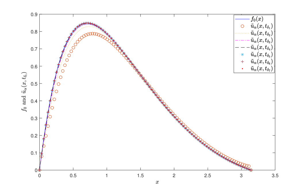
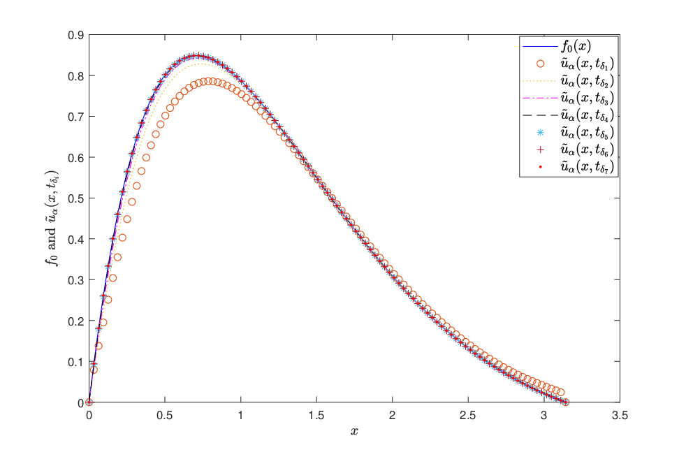
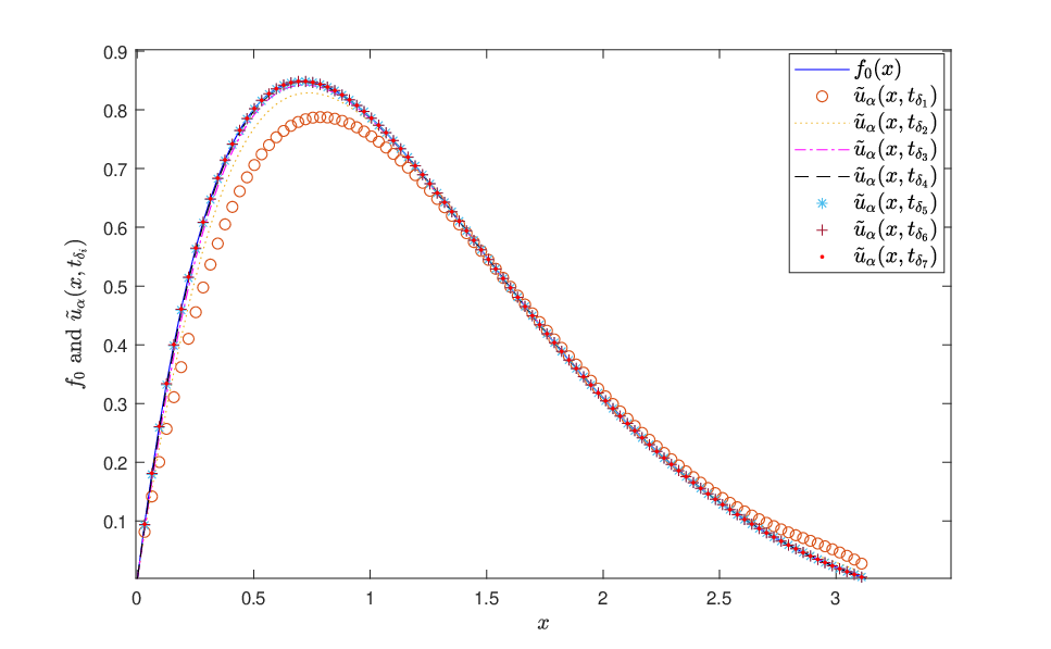
Taking δi=10−(i+2),i=1,2,…,7\delta_{i}=10^{-(i+2)},i=1,2,\ldots,7 we compute the exact expression f0f_{0} as well as u~α​(x,tδi)\tilde{u}_{\alpha}(x,t_{\delta_{i}}) and show them in Figures 55 to 88 for various α∈{0.2, 0.4, 0.6, 0.8}\alpha\in\left\{0.2,\;0.4,\;0.6,\;0.8\right\}.

Refer to caption
Figure 5. Solution profiles of f0​(x)f_{0}(x) and u~α​(x,tδi)\tilde{u}_{\alpha}(x,t_{\delta_{i}}) for α=0.2\alpha=0.2
Refer to caption
Figure 6. Solution profiles of f0​(x)f_{0}(x) and u~α​(x,tδi)\tilde{u}_{\alpha}(x,t_{\delta_{i}}) for α=0.4\alpha=0.4
Refer to caption
Figure 7. Solution profiles of f0​(x)f_{0}(x) and u~α​(x,tδi)\tilde{u}_{\alpha}(x,t_{\delta_{i}}) for α=0.6\alpha=0.6
Refer to caption
Figure 8. Solution profiles of f0​(x)f_{0}(x) and u~α​(x,tδi)\tilde{u}_{\alpha}(x,t_{\delta_{i}}) for α=0.8\alpha=0.8

In Table 22, we show the error ‖u~α​(⋅,tδ)−f0‖L2\|\tilde{u}_{\alpha}(\cdot,t_{\delta})-f_{0}\|_{L^{2}} for different values of α\alpha and δi,i=1,2,…,7\delta_{i},i=1,2,\ldots,7. Note that when δ\delta value decreases, the error ‖u~α​(⋅,tδ)−f0‖L2\|\tilde{u}_{\alpha}(\cdot,t_{\delta})-f_{0}\|_{L^{2}} decreases. This validates our theoretical result in Theorem 6.3.

Table 2. L2L^{2}-errors between f0f_{0} and u~α​(⋅,tδi)\tilde{u}_{\alpha}(\cdot,t_{\delta_{i}}) for α=0.2, 0.4, 0.6\alpha=0.2,\;0.4,\;0.6 and 0.80.8
α=0.2\alpha=0.2 α=0.4\alpha=0.4 α=0.6\alpha=0.6 α=0.8\alpha=0.8
δi\delta_{i} value ‖u~α​(⋅,tδ)−f0‖L2\|\tilde{u}_{\alpha}(\cdot,t_{\delta})-f_{0}\|_{L^{2}} ‖u~α​(⋅,tδ)−f0‖L2\|\tilde{u}_{\alpha}(\cdot,t_{\delta})-f_{0}\|_{L^{2}} ‖f0−u~α​(⋅,tδ)‖L2\|f_{0}-\tilde{u}_{\alpha}(\cdot,t_{\delta})\|_{L^{2}} ‖u~α​(⋅,tδ)−f0‖L2\|\tilde{u}_{\alpha}(\cdot,t_{\delta})-f_{0}\|_{L^{2}}
10−310^{-3} 8.2528(-2) 8.6054(-2) 8.6816(-2) 8.3284(-2)
10−410^{-4} 3.2857(-2) 3.4183(-2) 3.4288(-2) 3.2853(-2)
10−510^{-5} 1.1881(-2) 1.2337(-2) 1.2327(-2) 1.1816(-2)
10−610^{-6} 4.0572(-3) 4.2074(-3) 4.1935(-3) 4.0215(-3)
10−710^{-7} 1.3385(-3) 1.3870(-3) 1.3802(-3) 1.3240(-3)
10−810^{-8} 4.3110(-4) 4.4651(-4) 4.4386(-4) 4.2573(-4)
10−910^{-9} 1.3645(-4) 1.4123(-4) 1.4027(-4) 1.3453(-4)

Acknowledgement:   The first author M. Thamban Nair gratefully acknowledges the support received from BITS Pilani, K.K. Birla Goa Campus, where he is a Visiting Professor from August 1, 2023 after superannuation from I.I.T. Madras, Chennai.

References

  • [1] Duc Dang T, Huy Nguyen T. Regularization and error estimates for nonhomogeneousbackward heat problems. Electron. J Differ Equ. 2006; 2006:1–10
  • [2] H.W. Engl, M. Hanke and A. Neubauer, Regularization of Inverse Problems, Kluwer Acad. Publ., Dordrecht, Boston, London, 1996.
  • [3] Dinh Nho Hào, Jijun Liu, Nguyen Van Duc and Nguyen Van Thang, Stability results for backward time-fractional parabolic equations, Inverse Problems 35 (2019) 125006 (25pp)
  • [4] H. J. Haubold, A. M. Mathai, and R. K. Saxena, Mittag-Leffler functions and their applications, Journal of Applied Mathematics Volume 2011, Article ID 298628, 51 pages, doi:10.1155/2011/298628
  • [5] K. Jayakumar and M.T. Nair, Fourier truncation method for the non homogeneous time fractional backward heat conduction problem, Inverse Probl. Sci. Eng. 28 (2020), no. 3, 402–426.
  • [6] J.J. Liu and M. Yamamoto, A backward problem for the time fractional diffusion equation, Appl. Anal., 2010; 89:1769–1788.
  • [7] M.Thamban Nair, Functional Analysis: A First Course, Second Edition, PHI-Learning, New Delhi, 2021.
  • [8] M.Thamban Nair, Linear Operator Equations: Approximation and Regularization, World Scientific, 2009.
  • [9] Podlubny I. Fractional differential equations, San Diego: Academic Press; 1999.
  • [10] Akbar R. Safarov, Estimates for Mittag-Leffler functions with smooth phase depending on two variables, arXiv-math, 23 May 2022.
  • [11] Nguyen Huy Tuan, Le Dinh Longa, Van Thinh Nguyen and Thanh Tran, On a final value problem for the time-fractional diffusion equation with inhomogeneous source, Inverse Problems in Science and Engineering, Volume 25, 2017 - Issue 9