Prediction of Time and Distance of Trips Using Explainable Attention-based LSTMs
Abstract
In this paper, we propose machine learning solutions to predict the time of future trips and the possible distance the vehicle will travel. For this prediction task, we develop and investigate four methods. In the first method, we use long short-term memory (LSTM)-based structures specifically designed to handle multi-dimensional historical data of trip time and distances simultaneously. Using it, we predict the future trip time and forecast the distance a vehicle will travel by concatenating the outputs of LSTM networks through fully connected layers. The second method uses attention-based LSTM networks (At-LSTM) to perform the same tasks. The third method utilizes two LSTM networks in parallel, one for forecasting the time of the trip and the other for predicting the distance. The output of each LSTM is then concatenated through fully connected layers. Finally, the last model is based on two parallel At-LSTMs, where similarly, each At-LSTM predicts time and distance separately through fully connected layers. Among the proposed methods, the most advanced one, i.e., parallel At-LSTM, predicts the next trip’s distance and time with 3.99 error margin where it is 23.89 better than LSTM, the first method. We also propose TimeSHAP as an explainability method for understanding how the networks perform learning and model the sequence of information.
Keywords Trip prediction Attention LSTM Parallel LSTM Explainability TimeSHAP
1 Introduction
Trip prediction constitutes an important element for intelligent transport in various ways, e.g., simulation of public transportation, traffic analysis, battery charge planning, demand and load investigation, and preparation of vehicles for trips [7, 10, 8, 24, 6]. It also helps to optimize energy management, save energy, prolong components’ lifetime, and can also be used to support electric power systems [2, 3]. In particular, it yields increasing efficiency and reduces the energy consumption of Electric Vehicles (EVs) and even combustion engines.
Predicting the trip time can help prepare the vehicle for the mission by thermally conditioning the passengers’ cabin. This is specifically important for batteries or engines to avoid a cold start. In an electric vehicle, cold start may cause a reduction in the efficiency leading to capacity degradation of batteries and, subsequently, a reduction in their lifetime [16, 22, 17, 18].
Distance prediction can help to estimate how much energy will be needed. Also, it can pinpoint if warming batteries before the trip is needed by trading off energy efficiency, battery lifetime, and power availability. Knowing the amount of power needed for the trip can help to optimize charging policies and avoid fast charging, which may be used to take preventive measures for fast battery degradation [1, 23]. Using the information on both time and distance of trips can open the possibility of using batteries for the power flow in electric grid management [9, 11] and reduce energy consumption. It can also be used to plan to build charging stations in the cities, especially in megacities. Observing and predicting the general traveling pattern of vehicle users in a region can help to estimate the overall statistics of a transportation system.
Reaching all the accomplishments mentioned above highly relies on the possibility of predicting the accurate and exact time and distance of future travels. However, passengers do not always travel according to a linear planning schedule, and the trips can be made according to stochastic patterns. This stochasticity may even increase when predicting a fleet of vehicles. Several works have been proposed to predict the possible destination for a trip/vehicle [19, 12, 13, 7, 10] and the path/route to be taken under different conditions [2, 3, 4]. However, the prediction of the exact time of the trip and the distance that the vehicle will travel are not studied. In this paper, we develop two approaches to address this task. We propose predicting future trips’ time and distance by analyzing historical data using unique features-specific learning models based on LSTM and attention-based LSTM (At-LSTM) neural networks. We also develop timeSHAP, a posthoc model-agnostic explainability method specifically tailored for LSTM and At-LSTM handling multidimensional and length-variant sequences of information.
The contributions of this paper can be summarized as follows: i) We develop a novel deep learning-based framework utilized by At-LSTM-based structure to predict future trip time and distance that car will travel. ii) Using the most advanced method, the prediction error significantly decreases by about compared to using only LSTM. iii) The proposed method has minimal preprocessing steps and is a data-driven approach with a diverse dataset obtained from 700 vehicles. iv) we also develop timeSHAP as a model-agnostic LSTM explainer that is utilized based on KernelSHAP and expands it to analyzing sequential data. The rest of the paper is organized as follows: In section 2, we introduce the data, the four different models as well as the explainability component. In section 3, we demonstrate the experiments and discuss the respective results. Finally, we conclude the paper in section 4.
2 Methodology
In this section, we describe four different methods, including two LSTM based and two At-LSTM-based networks, as four solutions to predict the time of future trips together with the possible distance that will be traveled by the vehicle.
2.1 Data and preprocessing
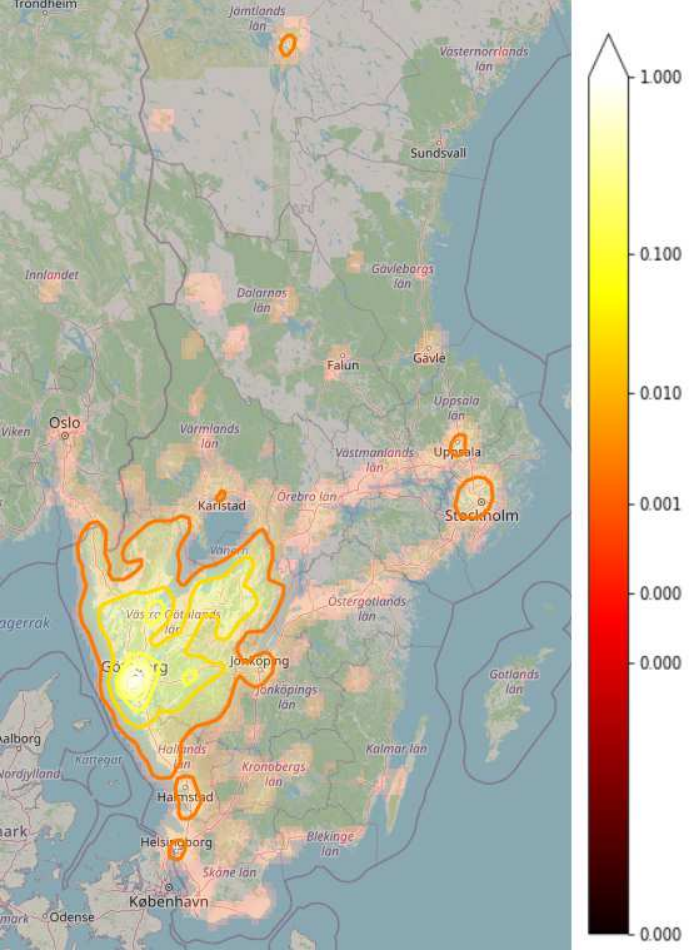
The dataset used in this study is a real-world dataset where 95962 trips have been collected by 700 GPS-tracked vehicles in Sweden. To avoid GPS disconnection, trips made within 10 min are considered one trip. Furthermore, the trips shorter than 3 km are discarded since the cold start of the vehicles are more energy efficient for short-distance travels. After applying such preprocessing steps, about of the original trips and of the vehicles are included in the filtered dataset. The density map of the trips based on GPS coordinates and the destination is illustrated in Fig. 1. More detail about the trips can be found in [15].
We define as in how many seconds the next trip will be made, i.e.,
| (1) |
where and are the time of the last two trips in historical data. We also define as the distance the vehicle has traveled. Finally, to consider the possibility of variation of the trip frequency on different days of the week, we consider the corresponding weekday as a feature alongside and . Therefore prediction of the future trip time and distance by observing the historical data can be formulated as follows.
| (2) |
where represents, for example, a deep learning model.


2.2 LSTM based methods
The first method (called ) consists of three LSTM layers followed by two fully connected layers (see Fig. 2 (a)). The input to the LSTM networks is a multidimensional matrix introduced in Eq. (2). The second method is based on using two parallel LSTM-based neural networks where each branch of the network receives separate and , and the outputs of the two LSTMs are then concatenated through two fully connected layers. Fig. 2 (b) illustrates the structure of the second method (called ). The third method (called ) is the attention version of the LSTM-based model developed in . Furthermore, due to the inequality of the length of the selected sequences of the trips, we use an embedding layer to equalize the length of the state vector for each LSTM layer and feed them to the attention layer. The structure of is shown in Fig. 3 (a). Finally, the last method is the attention-based version of the , where two parallel LSTM networks are processing and separately. Furthermore, the outputs of the LSTM layers go to separate attention layers, after which they are embedded using the embedding layer again. Finally, the outputs of the LSTM and attention layers are fed into a fully connected layer. Fig. 3 (b) illustrates the last method, called .
In the following, we describe the fundamental components of these methods, such as LSTM networks, embedding, and attention layer. In addition, we augment the models with an explainability component, as described thereafter.
2.2.1 LSTM networks
An LSTM cell, as a stateful operator, is a type of RNN that analyzes the and the distance of the trips sequentially [14]. For the sake of simplicity, we represent and , the input vectors to LSTM, together by , where is the length of the sequence. For each , is used to compute an output and updates the internal state of the cell at each layer which can be defined as:
| (3) |
where is a new state and is a nonlinear function parameterized by a set of weights . implicitly encodes the learned representation of the non-linearity and time-variance of the modeled data. For the LSTM cells, the exact update rules for and are defined in (4)-(6).
| (4) |
| (5) |
| (6) |
where is the input gate to write information into the cell, is the forget gate that receives the data for resetting the cell state, determines the magnitude of the influence of the input on the cell and represents the output gate which controls the information flow to the next layer. and are non-linear activation functions necessary for modelling non-linear data and is element-wise multiplication. All these cells, in combination, provide a powerful tool to learn features and model the behavior of time-variant data in order to be used as a predictor. The parallel version of the LSTM method in the mathematical derivation is illustrated in Algorithm (I).


: the distance that a vehicle travels on each trip
1
: time difference of the trip from the previous trip
2
Read (, , ,…, )
3
Max-min normalization of data 4
8
LSTM Networks 2 (for prediction of )
9
input gate
forget gate
output gate
cell information
state goes to next layer 11
12
input gate
forget gate
output gate
cell information
state goes to FC layer 13
Second FC layer:
18
2.2.2 Attention-based version of LSTM
The standard LSTM cannot detect which part of the sequence is relevant for aspect-level forecasting. In order to address this issue, we design an attention-based mechanism that can capture the key part of historical data in response to a given aspect. Fig. 3 (a) represents the architecture of this At-LSTM model.
Let be a matrix consisting of hidden vectors that the LSTM produces, where is the size of hidden layers and is the length of the given sentence. Furthermore, represents the embedding of both the aspect and vectors. The attention mechanism produces an attention weight vector and a weighted hidden representation , as follows.
| (7) |
| (8) |
| (9) |
where and are projection parameters. is a vector consisting of attention weights and is a weighted representation of produced by LSTMs. The operator in means that the operator repeatedly concatenates for times, where is a column vector with samples. is repeating the linearly transformed as many times as there are data points in the selected window of data. The last state representation can be defined as:
| (10) |
where, and are the weights to be inferred during training. Motivated from [20], we find that this model works practically better if we add into the final representation of the sequence of information.
The attention mechanism helps the model to apprehend the essential part of the information in the selected window of historical data where diverse characteristics are assessed.The parallel version of the LSTM method in the mathematical derivation is illustrated in Algorithm (II)
: the distance that a vehicle travels on each trip
1
: time difference of the trip from the previous trip
2
Read (, , ,…, )
3
Max-min normalization of data 4
8
LSTM Networks 2 (for prediction of )
9
input gate
forget gate
output gate
cell information
state goes to next layer 11
12
input gate
13
output gate
cell information
14
end while 16
19
Second FC layer:
21
2.3 Explainability
Here, we develop an explainer that is not only model-agnostic and post-hoc, but also specifically tailored to the At-LSTM networks. To be able to explain the predictor algorithm, the method must provide both trip and attributions of extracted features throughout the selected window of the sequence from historical data. The aim is to provide explainability of the sequential analysis while maintaining three desirable properties: accuracy, missingness, and consistency [21]. Therefore, we use an explainable, model-agnostic At-LSTM that is developed based on the TimeSHAP method introduced in [5]. TimeSHAP defines a significance index to the features or trips in the input that specifies the extent to which those features or trips impact the prediction task. To describe a piece of sequential information, , with trips and features of each trip, TimeSHAP fits a linear function (explainer) that matches the local output of a complex explainer by minimizing the loss function defined in [5].
The function that approximates is denied as
| (11) |
where the term is a bias value and resembles the output model with trips and features ticked off (dubbed base score). The set refers to the weights representing the impact of each trip/feature ( or ), for each dimension that is going to be explained. The perturbation function maps a coalition to the original input space . Note that the sum of significance indices for all the features corresponds to the difference between the score of the model and the score which is .
3 Experimental Results
In this section, we investigate the different models and compare their performances on our real-world dataset. We perform grid-search-based hyperparameter tuning for all methods to set their hyperparameters.
Considering the training time for each hyperparameter choice, we have selected 25 of data divided into test and training parts. The hyperparameters are aimed tuned, where the range of the search, steps on each search, and the corresponding results are shown in Table 1. As can be seen, the choice of the window of data, LSTM structure in all methods, and learning rate have the highest variation effect on the prediction error.
| hyperparameters | best value | P.err. Var.() | |
| LSTM | window size (1:1:14 days) | 5 | 23.8 |
| LSTM layers (1:1:5) | 3 | 18 | |
| neurons in LSTM layers (20:10:150) | 60,120,60 | 19 | |
| FL layers (1:1:3) | 2 | 3 | |
| batch size (16:16:512) | 128 | 5.2 | |
| lr (0.00001:0.05:0.1) | 0.01 | 17 | |
| optimizer (SGD, Adam, Adagrad, RMSProp) | Adam | 6.5 | |
| Loss (MAE, MSE, LHC, HL, MSLE, PS) | MAE | 7.3 | |
| Parallel LSTM | window size (1:1:14 days) | 8 | 25.8 |
| LSTM layers (1:1:5) | 3 | 15 | |
| neurons in LSTM layers (20:10:150) | 40,60,40 | 10 | |
| FL layers (1:1:3) | 2 | 3 | |
| batch size (16:16:512) | 128 | 6 | |
| lr (0.00001:0.05:0.1) | 0.01 | 19 | |
| optimizer (SGD, Adam, Adagrad, RMSProp) | Adam | 5.3 | |
| Loss (MAE, MSE, LHC, HL, MSLE, PS) | MAE | 10.3 | |
| Attention based LSTM | window size (1:1:14 days) | 8 | 25.8 |
| LSTM layers (1:1:5) | 3 | 15 | |
| neurons in LSTM layers (20:10:150) | 60,90,60 | 23 | |
| neurons in LSTM attention (4:4:256) | 64 | 21 | |
| FL layers (1:1:3) | 2 | 3 | |
| batch size (16:16:512) | 128 | 5 | |
| lr (0.00001:0.05:0.1) | 0.01 | 17 | |
| optimizer (SGD, Adam, Adagrad, RMSProp) | Adam | 6.2 | |
| Loss (MAE, MSE, LHC, HL, MSLE, PS) | MAE | 12.3 | |
| Parallel Attention based LSTM | window size (1:1:14 days) | 8 | 25.8 |
| LSTM layers (1:1:5) | 3 | 15 | |
| neurons in LSTM layers (20:10:150) | 40,60,40 | 10 | |
| neurons in LSTM attention (4:4:256) | 64 | 10 | |
| FL layers (1:1:3) | 2 | 3 | |
| batch size (16:16:512) | 128 | 5 | |
| lr (0.00001:0.05:0.1) | 0.01 | 17 | |
| optimizer (SGD, Adam, Adagrad, RMSProp) | Adam | 6.2 | |
| Loss (MAE, MSE, LHC, HL, MSLE, PS) | MAE | 12.3 |
| Scenario Methods | single LSTM | Parallel LSTM | At-LSTM | Parallel At-LSTM |
|---|---|---|---|---|
| Pred. Err. () for | 26.91 | 12.76 | 13.32 | 4.31 |
| 70 () Training 15 () Val. | ||||
| 15 () Test | ||||
| Pred. Err. () for Cross Val. | 26.01 | 10.97 | 12.49 | 3.99 |
Note that the evaluation of the performance of the proposed methods is based on the prediction error we obtained using, defined as:
| (12) |
where is the true value (label) and is the predicted value.
We perform our experiments Python environment using a workstation with an Intel i7 3.40 GHz CPU, 48GB RAM, and two NVIDIA GeForce RTX 4080 GPUs.
3.1 Comparison of different methods
Once all the hyperparameters are tuned, we train the networks in two ways. In the first scenario, we divide the data into three subsets: 70 for training, 15% for validation, and 15% for testing. In the second scenario, rather than having a fixed dataset for training and validation, we use cross-validation to train the neural network on each method. We randomly choose 75 of the data for training and 15 for 10 times. At each training, the weights of the previously trained networks will be updated when seeing a new dataset. Note that the test dataset is never used in the cross-validation process and is the same dataset used as test data for the first case scenario. We observe that cross-validation-based transfer learning improved the prediction accuracy for all methods (see Table 2). The convergence of the learning procedure is illustrated in Fig. 4 indicates the prediction error on the training and test dataset per epoch. As an example of the performance of the proposed methods, we illustrate the prediction of the distance of the trips on the part of the test dataset in Fig. 5. To avoid cluttering the results, only the LSTM and parallel At-LSTM method predictions are illustrated where they yield the highest and lowest prediction error, respectively. The blue line is the true labels, the red dashed line is the prediction using parallel At-LSTM, and the yellow dotted line is the prediction of true labels by the LSTM method. Observing the prediction results in Fig. 5, we conclude that parallel At-LSTM indeed performs better in the case of seldom trip patterns, whereas, in the repetitive patterns, pure LSTM yields a similar quality. Thus, this can be why the prediction accuracy of parallel At-LSTM is higher than the other methods developed in this paper.


3.2 Explainability
As described before, timeSHAP provides local explanations for the model’s behavior regarding a prediction. These descriptions can help improve the model in several aspects, such as auditing or model refining. Nevertheless, end-users, the fraud analysts, can mainly utilize the timeSHAP results to assist their decision-making. It can also be used to gather information and KPIs from end users to develop more sophisticated methods, such as online learning. The result of using the TimeSHAP method for the explainability of the performance of the networks can be seen in Fig. 6. We select two sequences: (i) we observe the trip from 1-49 and predict the trip number 50, and (ii) we observe trips 5-54 and predict the tip number 55. We extract timeSHAP values for historical trips in both scenarios. Doing such, indicates the contribution of each trip in the prediction task. Therefore, we can observe the performance of the proposed methods on how well they have learned the relevant patterns in the dataset for an accurate or inaccurate prediction. Considering the fact that the output of all methods is almost the same for scenario (i), to avoid cluttering the results, we only illustrate the timeSHAP values for the parallel At-LSTM method (see Fig. 6 (a)). As can be seen from the prediction of the distance of trip number 55, which has a true distance of 5.3 km, the information of trips 51 and 19 (pointed out with red-dotted arrows) have the highest timeSHAP values. Whereas the trips with distances above 50 km have negative timeSHAP value (see blue dot-dashed arrow). However, in scenario (ii), the timeSHAP values differ as prediction accuracy is significantly low for the LSTM method compared to parallel At-LSTM. Observing the timeSHAP values for both methods in Fig. 6 (b), the trips around 42-45, which are the longest in the distance, have the highest contribution to the prediction of trip 49. On the other hand, the trips with low distances have the least contribution to the prediction. On the other hand, observing the extracted timeSHAP values for the LSTM method in scenario (ii), the trips with the highest distance have a low contribution, and trips with a low distance have the highest contribution. This can be a reason why the prediction accuracy of LSTM is lower compared to the parallel At-LSTM method.
Thereby, we observe that the explainability method is able to successfully suggest the reasoning behind an accurate prediction. Furthermore, we can also see that the parallel At-LSTM has learned the historical patterns for predicting the future trip distance (). Finally, it may be concluded that the statement "the standard LSTM cannot detect which is the sequence part for aspect-level sentiment forecasting" is true in this setup.


4 CONCLUSION
In this paper, we proposed a novel deep learning framework for predicting the future distance and time of vehicle trips. We showed that the parallel attention-based LSTMs yield minimal prediction error compared to using only LSTM, attention-based LSTM, and two parallel LSTMs. This method outperformed the alternatives in terms of robustness and learning complicated patterns. Moreover, we developed a timeSHAP-based explainability method to show how the patterns have been learned by a method. Also, we observed that tuning the parameters and hyperparameters, such as choosing the number of days, features for creating sequences, or the learning rate of the optimization algorithms, can affect the prediction accuracy. Thus, it can be concluded that for an accurate predictor model, four important steps need to be followed: the art of feature selection, feature engineering, innovative selection and structuring of neural networks, and hyperparameter optimization of the machine learning methods. In future work, we are planning to create vehicle-specific models where the result of such can create a mother and universal model by using federated learning approaches.
References
- [1] Influence of plug-in hybrid electric vehicle charging strategies on charging and battery degradation costs. Energy Policy, 46:511–519, 2012.
- [2] Niklas Åkerblom, Yuxin Chen, and Morteza Haghir Chehreghani. An online learning framework for energy-efficient navigation of electric vehicles. In Proceedings of the Twenty-Ninth International Joint Conference on Artificial Intelligence, IJCAI, pages 2051–2057, 2020.
- [3] Niklas Åkerblom, Yuxin Chen, and Morteza Haghir Chehreghani. Online learning of energy consumption for navigation of electric vehicles. Artificial Intelligence, 317:103879, 2023.
- [4] Niklas Åkerblom, Fazeleh Sadat Hoseini, and Morteza Haghir Chehreghani. Online learning of network bottlenecks via minimax paths. Machine Learning, 112(1):131–150, 2023.
- [5] João Bento, Pedro Saleiro, André F Cruz, Mário AT Figueiredo, and Pedro Bizarro. Timeshap: Explaining recurrent models through sequence perturbations. In Proceedings of the 27th ACM SIGKDD Conference on Knowledge Discovery & Data Mining, pages 2565–2573, 2021.
- [6] Malte Bieler, Anders Skretting, Philippe Büdinger, and Tor-Morten Grønli. Survey of automated fare collection solutions in public transportation. IEEE Transactions on Intelligent Transportation Systems, 2022.
- [7] Yuxin Chen and Morteza Haghir Chehreghani. Trip prediction by leveraging trip histories from neighboring users. In 25th IEEE International Conference on Intelligent Transportation Systems, ITSC, pages 967–973. IEEE, 2022.
- [8] Boris Chidlovskii. Improved trip planning by learning from travelers’ choices. In MUD@ ICML, 2015.
- [9] Hugo Neves de Melo, João Pedro F. Trovão, Paulo G. Pereirinha, Humberto M. Jorge, and Carlos Henggeler Antunes. A controllable bidirectional battery charger for electric vehicles with vehicle-to-grid capability. IEEE Transactions on Vehicular Technology, 67(1):114–123, 2018.
- [10] Victor Eberstein, Jonas Sjöblom, Nikolce Murgovski, and Morteza Haghir Chehreghani. A unified framework for online trip destination prediction. Machine Learning, 111(10):3839–3865, 2022.
- [11] Mehrdad Ehsani, Milad Falahi, and Saeed Lotfifard. Vehicle to grid services: Potential and applications. Energies, 5(10):4076–4090, 2012.
- [12] Jonathan P Epperlein, Julien Monteil, Mingming Liu, Yingqi Gu, Sergiy Zhuk, and Robert Shorten. Bayesian classifier for route prediction with markov chains. In 2018 21st International Conference on Intelligent Transportation Systems (ITSC), pages 677–682. IEEE, 2018.
- [13] Alireza Ermagun, Yingling Fan, Julian Wolfson, Gediminas Adomavicius, and Kirti Das. Real-time trip purpose prediction using online location-based search and discovery services. Transportation Research Part C: Emerging Technologies, 77:96–112, 2017.
- [14] Klaus Greff, Rupesh K Srivastava, Jan Koutník, Bas R Steunebrink, and Jürgen Schmidhuber. Lstm: A search space odyssey. IEEE transactions on neural networks and learning systems, 28(10):2222–2232, 2016.
- [15] Sten Karlsson. The swedish car movement data project final report. Technical report, Chalmers University of Technology, 2013.
- [16] Soohwan Kim, Hoyoung Jeong, and Hoseong Lee. Cold-start performance investigation of fuel cell electric vehicles with heat pump-assisted thermal management systems. Energy, 232:121001, 2021.
- [17] Haitao Min, Zhaopu Zhang, Weiyi Sun, Zhaoxiang Min, Yuanbin Yu, and Boshi Wang. A thermal management system control strategy for electric vehicles under low-temperature driving conditions considering battery lifetime. Applied Thermal Engineering, 181:115944, 2020.
- [18] Paul Nelson, Dennis Dees, Khalil Amine, and Gary Henriksen. Modeling thermal management of lithium-ion pngv batteries. Journal of Power Sources, 110(2):349–356, 2002.
- [19] Ghazaleh Panahandeh. Driver route and destination prediction. In 2017 IEEE Intelligent Vehicles Symposium (IV), pages 895–900. IEEE, 2017.
- [20] Tim Rocktäschel, Edward Grefenstette, Karl Moritz Hermann, Tomáš Kočiskỳ, and Phil Blunsom. Reasoning about entailment with neural attention. arXiv preprint arXiv:1509.06664, 2015.
- [21] LLOYD SHAPLEY. A value for n-person games. contributions to the theory of games ii, kuhn, h., tucker, a, 1953.
- [22] Ayaka Shigemoto, Takuma Higo, Yuki Narita, Seiji Yamazoe, Toru Uenishi, and Yasushi Sekine. Elucidation of catalytic no x reduction mechanism in an electric field at low temperatures. Catalysis Science & Technology, 2022.
- [23] Matthew Shirk and Jeffrey Wishart. Effects of electric vehicle fast charging on battery life and vehicle performance. SAE Technical Paper 2015-01-1190, 4 2015.
- [24] Chunjie Zhou, Pengfei Dai, and Zhenxing Zhang. Orientsts-spatio temporal sequence searching for trip planning. International Journal of Web Services Research (IJWSR), 15(2):21–46, 2018.