Towards Black-Box Parameter Estimation
Amanda Lenzi11 1 School of Mathematics, University of Edinburgh, Edinburgh EH9 3FD, Scotland, United Kingdom. and Haavard Rue22 2 Statistics Program, King Abdullah University of Science and Technology, Thuwal 23955-6900, Saudi Arabia.
Abstract
Deep learning algorithms have recently been shown to be a successful tool in estimating parameters of statistical models for which simulation is easy, but likelihood computation is challenging. This is achieved by sampling a large number of parameter values from a distribution, which is typically chosen to be non-informative and cover as much of the parameter space as possible. However, for high-dimensional and large parameter spaces, covering all possible reasonable parameter values is infeasible. We propose a new sequential training procedure that reduces simulation cost and guides simulations toward the region of high parameter density based on estimates of the neural network and the observed data. Our following proposal aims to fit time series models to newly collected data at no cost using a pre-trained neural network with simulated time series of a fixed length. These approaches can successfully estimate and quantify the uncertainty of parameters from non-Gaussian models with complex spatial and temporal dependencies. The success of our methods is a first step towards a fully flexible automatic black-box estimation framework.
Keywords: Deep neural networks, intractable likelihoods, sequential, time-series, simulation
Short title: Black-box Estimation
1 Introduction
Statistical modeling consists of first devising stochastic models for phenomena we want to learn about and then to relate those models to data. These stochastic models have unknown parameters and the second step boils down to estimating these parameters from data through the likelihood function. However, there might be a discrepancy between these two steps, as models for describing mechanisms aim for scientific adequacy rather than computational tractability. Indeed, as soon as we move away from Gaussian processes as the canonical model for dependent data, likelihood computation becomes effectively impossible, and inference is too complicated for traditional estimation methods. Consider, for instance, datasets from finance or climate science, where skewness and jumps are commonly present and calculating the likelihood in closed form is often impossible, ruling out any numerical likelihood maximization and Bayesian methods. Yet it is computationally inexpensive to simulate from those models given parameter values, and the question becomes whether the simulations look like the data.
Much effort has been directed toward the development of approximate parameter estimation methods, often referred to as indirect inference (Gourieroux et al., 1993), likelihood-free inference (Grelaud et al., 2009; Gutmann and Corander, 2016), simulation-based inference (Nickl and Pötscher, 2010) or synthetic likelihood (Wood, 2010); for an overview, see, for example, the review by Hartig et al., 2011; Cranmer et al., 2020. The typical assumption by the different methods is that exact likelihood evaluation is hard to obtain but it is easy to simulate from the model given the parameter values, and the basic idea is to identify the model parameters which yield simulated data that resemble the observed data. The most common in this umbrella is arguably approximate Bayesian computation (ABC) (Fearnhead and Prangle, 2012; Frazier et al., 2018; Sisson et al., 2018), which avoids evaluating intractable likelihoods by matching summary statistics from observations with those computed from simulated data based on parameters drawn from a predefined prior distribution. The likelihood is approximated by the probability that the condition is satisfied, where is some distance measure and the value of is a trade-off between sample efficiency and inference quality. In simpler cases, sufficient statistics are used as they provide all the information in the data, however, for complex models they are unlike to exist and it is not obvious which statistics will be most informative. Several works have proposed procedures for designing summary statistics (Fearnhead and Prangle, 2012; Jiang et al., 2017), and a comparison of likelihood-free methods with and without summary statistics have been empirically tested in Drovandi and Frazier, 2022. Despite its popularity, ABC is not scalable to large numbers of observations since inference for new data requires repeating most steps of the procedure.
A recent line of research on likelihood-free inference uses deep learning to estimate parameters of statistical models. The first work to propose neural networks-based estimators in the statistical community focused on parameters of spatial covariance functions in Gaussian processes (Gerber and Nychka, 2020). They showed that convolutional neural networks (CNNs) can learn the mapping between data and parameters and had similar estimation accuracy and a considerable reduction in computational time compared to classical maximum likelihood estimators. Based on the same idea, Lenzi et al., 2021 estimated parameters of models for spatial extremes for which the likelihoods are intractable and, therefore, MLEs are unavailable. A modified parametric bootstrap approach was introduced to quantify the uncertainty in these estimators. Variants to those methods to incorporate replicated data in the estimation (Sainsbury-Dale et al., 2022), irregular spatial data (Sainsbury-Dale et al., 2023), and censoring information (Richards et al., 2023) were successfully recently introduced. Estimation in high dimensions and large parameter spaces is still an open question since constructing training data that covers all possible reasonable parameter values becomes quickly infeasible. An inevitable drawback of the current approaches is the estimator’s bias towards the parameter region of the training data. Whereas previous work simulated training data either with parameter values around the truth or based on inexact likelihood estimates, these methods are expensive and unrealistic. In this work, we solve the bias issue of previous methods with an automatic iterative approach that modifies the training data using arbitrary, dynamically updated distribution parameters until it reaches the parameter region corresponding to the actual data. The proposed inference mechanism automatically performs parameter estimation without restrictive assumptions about the generating process, knowledge from experts, or computationally expensive preliminary steps.
Various approaches have been proposed for guiding simulations by making use of the observed data. The sequential training procedure proposed here falls into a broader class of methods that seek to update the prior distribution to alleviate the curse of dimensionality that comes with having to explore a large volume of data when the number of parameters is large. Within ABC implementations, a Sequential Monte Carlo procedure was used to guide simulations based on previously accepted parameters (Sisson et al., 2007; Beaumont et al., 2009; Bonassi and West, 2015). Järvenpää et al., 2019; Lueckmann et al., 2019 updated simulations that reduce the Bayesian uncertainty in the posterior estimate. A sequential estimation procedure selected future simulations by proposing parameters from preliminary approximations to the posterior (Lueckmann et al., 2017; Papamakarios and Murray, 2016). Sequential approaches have been considered in the context of neural networks for learning a model of the likelihood in the region of high posterior density Papamakarios et al., 2019, but only for toy examples and small datasets. Our approach stands out from previous methods as it is aimed at point parameter estimation in intractable statistical models with large and complex datasets. We leverage our statistical knowledge about scaling data and parameters to reduce computational costs and improve convergence when training the neural networks. We first illustrate the new approach on a Gaussian toy example, where the intended coverage probability of the estimator is known, and further for modeling spatial extremes. Similarly to Papamakarios et al., 2019, which trains autoregressive flows on all simulations obtained up to each round rather than training only with simulations from the latest round, we broaden the range of the training by reusing training data from previous iterations. Consequently, most of the training data in later rounds still come from the most probable parameter regions, and the added simulations from previous rounds broaden the range of searches at no computational cost. We leverage the ideas of improving the estimator by updating the prior in multiple rounds. Since our approach is designed to yield precise point estimates instead of approximating posterior distributions, the loss function in the neural network remains independent of the current proposed prior. We apply the modified parametric bootstrap technique in Lenzi et al., 2021 such that in each round, the new approach is able to quantify both the bias and variance of the estimators. Our experimental results show that the sequential approach dramatically reduces the bias of an initial guess and eventually approximates the actual parameter quite accurately, even when the initial training does not contain the truth.
Our next contribution is designed to handle estimation for different data sizes originating from the same model. This is achieved by training a neural network only once on an extensive database and replicating the observations as needed to achieve the training data length before processing them on the pre-trained neural network. We adjust for the underestimation in the uncertainty of the replicated series by rescaling its sampling variance to match the original series variance. We apply this strategy to estimate parameters of non-Gaussian stochastic volatility models, which are widely used in finance. In such applications, where early access to results may carry a premium, our deep neural network (DNN) estimator is particularly advantageous since the network is trained beforehand, and estimates are obtained instantaneously when new data becomes available. This example shows that our estimator is well calibrated, with uncertainty quantification closely matching those from the state-of-the-art Integrated Nested Laplace Approximation (INLA) approach (Rue et al., 2009).
The remainder of this paper is organized as follows. First, Section 2 outlines the methodologies we develop for designing training data to train DNNs, along with some practical considerations. In Section 3, we introduce the construction of the automatic iterative approach and conduct simulation studies for Gaussian i.i.d and spatial extremes model, whereas in Section 4, we describe our unified database approach applied to time series data from an intractable model. In Section 5, we conclude and summarize avenues for future research.
2 Parameter estimation with DNNs
2.1 Background
Consider a dataset of observations generated from , where is a Lesbegue measure and denote the set of all Borel probability measures on the sample space . To describe such a process, it is common practice to assume a statistical model with probability density function parameterized by a finite number of parameters , which is estimated using the observations through the log-likelihood function .
Highly structured data coming from a high-dimensional are often related to intractable or computationally demanding likelihoods, but simulating data from for given parameters is usually trivial. Recently, parameter estimation using DNNs have opened doors to solving previously intractable statistical estimation problems. The key to efficiency is to avoid altogether learning likelihood functions and directly learn the mapping between data and parameters through DNNs by carrying out simulations. To formulate the problem, let be a simulated sample from with given parameters . Then, the mapping from onto is learned by adjusting the weights w and biases b, denoted by of a DNN , such that
| (1) |
Optimizing (1) with respect to requires the minimization of the loss function , which is chosen to reduce the error in prediction for a given output and simulated data . A popular choice in regression problems is the mean squared error (MSE)
Often, no closed-form solutions can be derived for the optimization in (1), and advanced numerical optimizers built around batch gradient descent methods are employed (Kingma and Ba, 2014). Finally, once the DNN has been trained, one can use the estimated to plug in into the trained DNN and retrieve , which will then output parameter estimates of interest .
2.2 Transformations to data and parameters
Here, we detail our rationale for choosing transformations to data and parameters and make the problem more palatable for the DNN. The key is to use our statistical knowledge of intrinsic data and parameter properties to leverage estimation. For instance, the quadratic loss in (2.1) is optimal for outputs with constant mean and variance that are a real-valued function of the inputs with Gaussian distributed noises. If these assumptions are met, the estimator retains the desired properties, such as the minimum variance and fast convergence, as the gradient reduces gradually for relatively small errors (Friedman et al., 2001). Therefore, reparametrization related to scaling should aim for a constant variance for different parameter values.
When minimizing the loss in (1), is usually initialized to random values and updated via an optimization algorithm, such as stochastic gradient descent based on training data. As is usually the case, the geometry of the surface that has to be optimized will be complicated and smooth due to an ample search space and noisy data, and using the raw data will likely result in slow and unstable convergence. To remedy this problem and improve the algorithm’s stability, one should aim for properties such as symmetric and unbounded distributions, orthogonal parameters, and constant Fisher information. The logarithm and square root transformations often used in time series problems are examples of desirable change that affects the distribution shape by reducing skewness, stabilizing the variance, and simultaneously avoiding boundaries. Parameterization with meaningful interpretations such as mean and variance should be preferred over directly using distribution parameters.
In Sections 3 and 4, we will use transformation within a DNN pipeline to estimate parameters of models for Gaussian data, spatial extremes, and non-Gaussian stochastic volatility models. We show that whereas these precautions are helpful in simple Gaussian examples, they are indispensable in complex models such as for spatial extremes.
2.3 Designing training data
Recall that the first step for optimizing (1) is generating pairs of training data . The main challenge here is to generate training data that correspond to configurations covering the parameter domain of the observations, which is unknown. Since is often unbounded and it is impossible to simulate over the entire domain. Not introducing an appropriate structure or prior scientific knowledge will lead to inaccurate training data and, thus, erroneous estimation.
In the context of intractable likelihoods for which MLEs are unavailable, Lenzi et al., 2021 proposed to simulate training data based on informative parameter estimates from approximate maximum likelihood methods fit to spatial extremes data. However, obtaining these estimates for every new dataset becomes problematic if likelihood estimation is slow or not feasible in the first place. Here, we propose two different strategies to deal with this challenge. The intuition behind these method goes as follow:
- (A)
A fully automatic iterative approach: Promising regions in are found sequentially. The DNN is initially trained with based on a crude guess (e.g., from a simpler model). The trained DNN then receives and outputs , which is used to simulate bootstrapping samples . Next, is fed into the trained DNN to output bootstrapping samples . The spread of and its distance from are used to guide simulations for training the DNN. Empirical results show a higher concentration of training data and bootstrapping samples around the true parameters after a few iterations, hence a better approximation of .
- (B)
A general unified database approach for time series: Computation efficiency is achieved by training the DNN in advance and reusing it to estimate newly collected data for free. The pre-training is based on an extensive database comprising simulated time series data and corresponding parameters . Next, parameter estimates from new data of different lengths are obtained by replicating the observations to achieve the size of .
3 A fully automatic iterative approach
3.1 General framework
We now use the notation in Section 2 to describe an algorithm that sequentially samples training data until it reaches the correct parameter regions from the data. Our algorithm is initialized with simulated pairs (, where the elements in are draw from independent Uniform distributions, each bounded below by and above by , while is data simulated with . Intervals may or may not contain the true parameter . Whereas good initial guesses of and are not essential here, most models allow for some data-driven estimates, e.g., based on simplified Gaussian assumptions. Next, a DNN is trained with (, and then used to retrieve estimates when fed with observations .
The main idea is to then dynamically update the training data ( by changing the values of and based on information on whether is underestimating or overestimating . For instance, if is close to the upper boundary of the training data for a specific , then new training samples should be expanded to contain data outside of that boundary. Information on the accuracy of is obtained by sampling new data with using , and feeding these data into the initially trained DNN producing a bootstrapped sample . For each , we then update and to values in a neighborhood of , where the neighborhood region is defined by the size of the bias between and , where is the median of , and the neighborhood width depends on the quantiles of the bias between the fitted value and the bootstrapped sample: , where is a quantile. The algorithm stops when the bias between and is sufficiently small compared to the standard deviation of , which we denote by , for all . In more detail, the algorithm is as follows.
Need: Observations from a distribution and a neural network
Pick , and
Small values of in line 1 of Algorithm 1 will make the algorithm run longer, since it requires to be closer to relative to the spread of . At each iteration, line 5 automatically provides uncertainty quantification of through . This step works as a modified and more efficient parametric bootstrap method since it uses the previously trained DNN, and no model fitting is required to produce . One can use these samples to compute quantities of interest, such as confidence intervals and coverage, and check the overall appropriateness of the method. Here, we use them to quantify the accuracy of the current iteration and to update the training data for the next round (see lines 6 and 7).
Parameter values are usually in the transformed scale, and we continuously sample training data such that the values in this transformed scale are uniformly distributed (see line 2 of Algorithm 1) rather than applying transformations after the training data have been generated to train the DNN. The former would produce regions of scarcity in , and results for testing data within the underrepresented values would not be optimal. Indeed, the optimization inside the DNN will perform best if the training data have no significant gaps between values, a problem also called imbalanced data in classification problems (Murphey et al., 2004).
In Section 3.2, we estimate the parameters of an i.i.d Gaussian model as a proof-of-concept, whereas, in Section 3.3, we consider a spatial-extremes setting and estimate the parameters of the Brown-Resnick max-stable process with an intractable likelihood. This procedure supports a wide range of likelihoods with fixed and random effects, and distributions other than the Uniform could also have been used in line 2 of Algorithm 1.
3.2 I.i.d. data
Although classical inference for the models considered in this section is straightforward, they allow us to compare our estimates’ accuracy and uncertainty with MLEs. For applications where our method is of practical interest, see Section 3.3. In what follows, we look at three problems of increasing complexity from parameters of Gaussian distributions: the logarithm variance (single parameter), the mean and the logarithm variance (two orthogonal parameters), and the first moment and logarithm of the second moment (two highly dependent parameters). With these examples, we aim to empirically illustrate that our framework: (1) approaches the MLE even when the initial training data is relatively far from the actual value, and (2) reaches the truth quicker when using meaningful parametrizations and orthogonal parameters.
Consider i.i.d. observations from a Gaussian distribution . We find that in line 1 of Algorithm 1 is enough to provide good estimation accuracy without overly increasing computational cost. Algorithm 2 shows the steps of our procedure for the i.i.d. case (see Algorithm 1 for the general case), whereas some practical aspects are discussed in what follows.
Need: Observations from a distribution and a neural network
Pick and
Multi-layer perceptron (MLP)
A perceptron is a single neuron model, and MLPs are the classical type of neural network comprised of one or more layers of several neurons. It takes 1D vectors as the input and learns nonlinear relationships between inputs and outputs, making it a suitable choice for our i.i.d. regression problem. Due to the simplicity of this toy example, we find that a small MLP with a single hidden layer and 50 hidden units is enough to near the mapping between data and parameters. We consider an MLP for taking output in and input in .
Progressively increasing training accuracy
Our algorithm uses fewer training samples when estimation uncertainty is larger, at the beginning of the algorithm, and more samples towards the end, when more precision is required. When the estimates are close to stabilizing, and the uncertainty has decreased, the number of samples in the training data is set to increase by (see line 8 of Algorithm 2).
Results for a single parameter
Figure 1 displays the results for estimating when the mean is known using Algorithm 2. We set and uniformly generate training output samples and corresponding inputs . The grey boxes in this figure are the training data at each iteration, whereas fitted values are represented by the red line, with the blue boxes showing bootstrapped estimates for . After five iterations, the algorithm approaches the MLE (green dashed line) with low uncertainty (see narrow blue boxes). To quantify the appropriateness of our method, we compare central intervals from the bootstrapping estimates with the same interval from the empirical variance in the data. The interval provides adequate uncertainty of the MLP estimates, with bootstrap interval on compared to for the intended coverage probability of the MLE.

Results for two independent/dependent parameters
We now increase the problem’s complexity and evaluate the performance of Algorithm 2 when two parameters are estimated jointly. We use the same test data as in the single parameter estimation case (see Figure 1), that is, data from a Gaussian distribution with and . Specifically, we look at two cases: 1. estimating the mean and log-variance and 2. estimating the first moment and the logarithm of the second moment . Whereas in case 1, the parameters are independent, the MLP has to learn the relation between data and highly dependent parameters in case 2. In both cases, initial training data does not contain the actual parameters, such that: 1. , and , 2. and . Similarly to the single parameter estimation, we fix and . Figure 2 displays the estimates for Case 1. (top row) and 2. (bottom row) after running Algorithm 2 with the logarithm transformations (left column) and without (right column). Estimates are more accurate when the parameters are transformed, and for Case 2, the MLP underestimates the raw moments. Especially for the second moment, the algorithm without transformation narrows the estimates close to the median of the initial training data. In contrast, the reparametrization is able to recover highly dependent parameters accurately. Indeed, in both cases, the MLP can detect accurate parameter estimates already in the first iteration. The subsequent iterations refine the estimates and concentrate the training and the bootstrapping samples around the MLEs. This experiment reiterates the benefit of using unbounded and orthogonal parameters for training the MLPs.


3.3 Spatial extremes
We now move to a more complex model for spatial extremes, which is well-known to have a likelihood function that is effectively impossible to compute. Max-stable distributions are the only possible non-degenerate limits of renormalized pointwise maxima of i.i.d random fields and, therefore, the most commonly used for studying multivariate extreme events Davison et al., 2012. We consider the following definition of a max-stable process
| (2) |
where are points of a Poisson process on with intensity . We consider the Brown-Resnick model (Kabluchko et al., 2009), which arises when . Each is a nonnegative stochastic process with unit mean, whereas are copies of a zero-mean Gaussian process with semivariogram , spatial separation distance , range , smoothness and such that .
The cumulative distribution of is
where satisfies homogeneity and marginal constraints. The full likelihood is written as
where is a collection of all partitions of and denotes the partial derivative of with respect to the variables indexed by . The full likelihood is intractable even for moderate since the number of terms grows equals the Bell number, which is more than exponentially. The standard workaround for this issue is to consider only pairs of possibly weighted observations in the likelihood (Padoan et al., 2010; Davis et al., 2013; Shang et al., 2015):
where is the block maximum at location , , is the vector of unknown parameters and is the weight of .
We compare the estimators from our fully automatic iterative approach with pairwise likelihood estimation on independent simulated datasets of a Brown-Resnick model with and on a spatial domain of size with unit-square grid cells. The steps used for estimating parameters of Brown-Resnick processes are shown in Algorithm 3. To improve accuracy and efficiency, the pairwise likelihood if fit only with pairs with at most 5-units apart and using the R-function fitmaxstab from the SpatialExtremes R-package (Ribatet, 2013).
Need: Observations from a distribution and a neural network
Pick and , and set
Convolution neural network (CNN)
CNN uses convolutions, that is, the application of a filter to the input image that results in what is called an activation. Repeated application of the same filter to images results in a map of activations (feature map). This map indicates the locations and strength of a detected feature in the input, such as the edges of objects, and therefore, it is a common choice for regularly-spaced gridded images. We use two 2D convolutions with 16 and 8 filters, respectively, and rectified linear unit (ReLU) activation function and kernel of size (Hastie et al., 2009). We add one dense layer at the end of the network with four units that map the input image to an output vector of size two. The CNN weights are initialized randomly and trained using the Adam optimizer (Kingma and Ba, 2014) with a learning rate of 0.01. The training is performed for 30 epochs, and at each epoch, the CNN weights are updated utilizing a batch size of 100 samples from the entire training dataset.
Initialization
We start the by simulating pairs , where and is simulated from (2). We initialize based on estimates of a Gaussian process with powered exponential covariance function , which closely matches the Brown-Resnick variogram. We sample . Such estimates are likely biased for Brown-Resnick, but they are quick to compute and a better start than a random guess. A line search for indicates that provides good results but found that other values of gave similar accuracy. We uniformly draw over approximately the whole (bounded) domain: . We initialize the pairwise likelihood with the powered exponential covariance function estimates for a fair comparison with our approach.
If the parameter region for simulating data at each iteration is tightened too quickly or shifted by too much, it may miss the true parameters. To alleviate this issue, we randomly select of the samples from the previous iteration that were not contained in the updated interval and add them to the training data of the current step (see line 9 of Algorithm 3). Besides increasing the size of the training without having to simulate new data, this broadens the range of the training while still keeping most of the samples in the updated region defined by the current step. Therefore, it prevents the current iteration from being stuck in the wrong region while maintaining more accurate training data in the most probable parameter region.
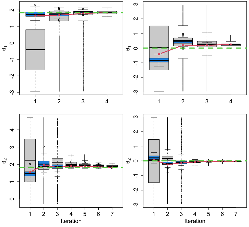
Figure 3 shows a scatterplot of 100 independent estimates of versus from the last iteration of our approach (green) and from the pairwise likelihood (red). The symbol is the truth. Whereas the proposed method produces robust results across the different replicates, the pairwise likelihood tends to underestimate the smoothness parameter, and the performance varies considerably across datasets. In Figure 4, we access the accuracy of Algorithm 3 for estimating (left column) and (right column) with boxplots. The rows in this figure illustrate the results for two different datasets: The first is initialized with training data that do not contain (top), whereas the variogram estimate for the second dataset is close to the center of the training data. Indeed, whereas the space covering is bounded, and simulating training data covering the entire region is straightforward, the training data for is based on the variogram estimate and, therefore, only sometimes contains the truth. The grey and blue boxplots at each plot and iteration are the training output and bootstrapping samples, respectively. As expected, the gray boxplots in all cases at iterations 2 and 3 contain several outliers, which correspond to the samples reused from the previous step. Points in the red line are the fitted values from the CNN, and the green dashed lines are the actual parameters used to simulate data.
Even when the true value is not included in the initial training data (see the top of Figure 4), the CNN estimates well and produces reasonable uncertainties. At the last iteration, the training data for both parameters are narrow and around the actual value, and the bootstrapping samples practically coincide with the training data. When initialized with training data containing the truth, the CNN quickly approaches the truth with low uncertainty for both parameters and remains stable until it reaches the stopping criteria. A quantitative measure of the effect of the iterations in Algorithm 3 is reported in Table 1, with bias, standard deviation, and root mean square error (RMSE) for the first and last iterations. The metrics are calculated from the bootstrapping samples among the 100 independent datasets. Point estimates are taken as the median of the bootstrapping samples. Under all three metrics, there is a considerable improvement from the first to the last iteration of the algorithm, and estimation at the last iteration are about more efficient for and more efficient for (with the efficiency defined as the ratio of RMSEs).

| Iteration | bias | sd | RMSE | bias | sd | RMSE |
| First | 0.223 | 0.295 | 0.563 | 0.005 | 0.253 | 0.451 |
| Last | 0.056 | 0.129 | 0.306 | 0.004 | 0.120 | 0.313 |
4 A general unified database approach for time series
4.1 General framework
Suppose we observe time series data from a strictly stationary process indexed on the temporal domain . Let be the probability distribution of depending on the parameter set . The stationarity assumption is that the joint probability distribution of does not depend on for any . This Markov property is common in time series analysis similarly with ergodicity, which provides the justification for estimating from a single sequence .
Our main goal is to estimate by training a DNN using parameter candidates as output and corresponding simulated data as input (see Section 2). Here, we take advantage of the stationarity property to generalize and improve the estimation workflow described in Section 2. Our approach is best exemplified by a toy data with from an AR process of order 1 with coefficient . Instead of simulating training data of length , we proceed by simulating time series of length and construct data pairs , where and and train a DNN. Next, since is shorter than the training data, we create a new time series by concatenating to achieve the length of the time series used during training. Figure 5 shows how to construct from by replicating the observations five times. The red dashed line are the joining points. The resulting is then fed into the trained DNN to retrieve estimates .

Recurrent neural networks take information from prior inputs to predict the current input and output and can handle sequence data and inputs of varying lengths by memorizing historical information. Therefore, these networks are unsuitable for our problem, as our output data does not have future sequence values. Here, we are interested in mapping parameters to sequential data rather than learning the next value in a sequence. As we will see in the example in the next section, our technique has several advantages over training the DNN using simulated data with the same length as the observations: (i) allows estimation of time series of several sizes at almost no computational cost, since the DNN does not have to be retrained for each new dataset, (ii) holds without requiring any particular dependence structure assumption as long as the data is stationary and Markov.
Connection to non-overlapping block bootstrap (NBB)
The intuition behind our approach resembles NBB approaches (Carlstein, 1986). Similarly, this technique splits the observations into non-overlapping blocks and resamples the blocks with replacement, which are replicated to obtain a bootstrapped series. However, unlike block bootstrap methods, where the complex problem of choosing the block size has to be solved, by construction, our block size is always fixed and equal to .
Discontinuity at the joining points
Our procedure of laying sequences of length end-to-end will inevitably produce discontinuity points where the joining occurs, similarly to what happens in bootstrap for time series. However, as we will show empirically in our examples, these discontinuities will have a negligible contribution to the model parameters structure.
Varying observation lengths
As long as the database for training the neural network is extensive enough, the proposed method is easily generalized for cases where is not a multiple of . If the observed time series is shorter than that used during training, that is , one can replicate the data into blocks, where , and complete the remaining values with a random block from of size . The idea is that if is large enough compared to and with , as and , the last components of have little influence in the dependence structure. On the other hand, if , we take the first observations and estimate parameters , the next and estimate , and so on. If the last sequence from this procedure is smaller than , we use the method for dealing with described previously. Next, we merge the results from these several estimates (e.g., by using the sample average) to create a single combined estimate , which can then be used to simulate bootstrap samples and construct confidence intervals.
Uncertainty quantification
To account for the underestimation in the uncertainty that results from applying the estimator to the replicated time series, we scale the sampling variance by the number of blocks used to replicate the original series. For instance, consider the simulated toy example in Figure 5 of an AR(1) process with and an AR coefficient . The MLE is , and its corresponding standard deviation is . If the series is then replicated times such that the new length is , the new MLE is not affected (), but its standard deviation is now . Therefore, to recover the correct uncertainty, we need to scale the new standard deviation by , that is, , which is then, approximately, the standard deviation of . This adjusts the uncertainty for the fact that no additional information is added to the replicated data.
1D Convolutional Neural Networks
Since we are dealing with parameters from time series data, we train 1D CNNs, which have proven successful in learning features from dependent observations onto one-dimensional dependent sequences. As for 2D CNNs (see Section 3.3 for an example), the input layer receives the (transformed) data, and the output layer is an MLP with the number of neurons equal to the number of output variables. Each neuron in a hidden layer first performs a sequence of convolutions, the sum of which is passed through the activation function followed by a sub-sampling operation. The early convolutional layers can be seen as smoothing the input vector, where the filters are similar to parameters of a weighted moving average but learned jointly with the regression parameters from the MLP layer. In what follows, we use three 1D convolutions with four filters each, the ReLU activation function, a kernel of size three, and one final dense layer with four units. We set a learning rate of 0.01 with 30 epochs and a batch size of 50 samples to update the weights.
4.2 Non-Gaussian stochastic volatility model
To show the usefulness of our approach, we focus on estimating parameters of financial time series data that exhibit non-Gaussian time-varying volatility. Volatility is highly right-skewed and bounded, making Gaussian distributions a poor representation. A better description of volatility is achieved with stochastic volatility models (SVOL), first introduced in Taylor, 1982 and currently central to econometrics and finance investments theory and practice. The idea of SVOL models is to parsimoniously fit the volatility process as a latent structure using an unconditional approach that does not depend on observations. We consider the following model structure
| (3) | ||||
where and are independent noises and is the number of observations. The volatility variable is latent with an AR(1) structure, and only is observed. When , is strictly stationary with mean and variance (Fridman and Harris, 1998).
Likelihood evaluation of continuous dynamic latent-variable models such as (3) requires the integration of the latent process out of the joint density, resulting in the following -dimensional integral
| (4) | ||||
where , , the conditional densities and have the form in (3), and the initial volatility is the stationary volatility distribution . Since is not independent from the past, the integral in (4) cannot be factored into a product of one-dimensional integrals and exact evaluation of the likelihood is possible only in special cases like when both and are Gaussian. Alternative approaches for likelihood evaluation include computationally demanding Markov Chain Monte Carlo (MCMC) (Andersen et al., 1999) and the more recent and faster Integrated Nested Laplace Approximation (INLA) (Martino et al., 2011).
Next, we give practical details of our framework as well as the a comparison of the results from our approach and the state-of-the-art INLA approach for estimating parameters of the SVOL model.
Implementation
Consider observations , from the SVOL model with , and . We use scaled (variance one) versions of both and in (3), such that only and need to be estimated. To show the effect of estimating time series of different lengths with a single DNN fit, we display the results for various time series lengths: . Estimation goes as follows. The training database contain samples pairs of transformed parameters , with and and corresponding data simulated from (3). The transformed parameters are sampled uniformly in a neighborhood of the actual parameter values and :
| (5) | ||||
New test data is obtained by replicating times as many time as needed to achieve size . We fix in (5) to ensure a large enough region around the true values, although other constants provided similar results.
Figure 6 displays scatterplots of estimated versus estimated from independent replicates of the SVOL model. Scatterplots from top to bottom, left to right, shows testing sets of different size: . Green dots are the 1D CNN estimates, and red dots are the mean of the predicted posterior distribution from fitting model (3) using INLA. The symbol in each plot represents the truth. As the testing data sizes increase, both methods concentrate the estimates around the truth, and the 1D CNN estimates are less variable and less biased for smaller values of ; after that, both methods seem to perform similarly well. Whereas we set the INLA priors to default values, changing them to penalize parameter values far from the mode could potentially improve the results.
To quantify the uncertainty in the 1D CNN estimates, we create a bootstrapped dataset by independently sampling time series from the fitted model and then feeding these samples into the trained 1D CNN. The uncertainty in the estimation of (left) and (right) from both methods is grasped in Figure 7. The bars represent central intervals, taken from the posterior distribution given by INLA (red) and the 1D CNN bootstrapped samples (blue) for one randomly chosen dataset among the replicates in Figure 6. The -axis represents different test data sizes , and the gray horizontal dashed line is the truth. As expected, the uncertainties decrease with sample sizes for both methods. The intervals from both methods are close for most data sizes, although the INLA distributions are more concentrated for and . Overall, these results show that the 1D CNN is robust to estimating parameters of different data lengths and in agreement with the INLA estimator.


5 Conclusion
We proposed approaches that train DNNs to estimate parameters of intractable models and quantify their uncertainty. Unlike previously proposed approaches using DNNs, which are tailored to a specific application and can lead to poor parameter estimates for relying on computationally expensive initial guesses to construct training data, our methods (A) leverage an iterative learning framework coupled with a modified parametric bootstrap step to guide simulations in the direction of the parameter region of the actual data in multiple rounds (B) use an extensive pre-trained database to accurately estimate parameters of time series data of multiple lengths at no computational cost, rather than simulating data for every new dataset.
Our estimators yield accurate parameter estimates with much less computation time than classical methods, even when accounting for the time required to generate training samples. The experiments discussed in this work involve models with a maximum of two parameters for clarity in presentation. We anticipate a more pronounced influence of our sequential approach in higher-dimensional scenarios for alleviating the challenges associated with the “curse of dimensionality” as the volume of the parameter space increases exponentially with the number of parameters.
While DNNs for parameter estimation are gaining popularity, we still need to learn more about black-box algorithms applied to previously intractable statistical problems and how to design task-specific estimators more generally. There are several further opportunities for exploring DNNs for parameter estimation using newly designed optimization tools from the machine learning community. This work is another step towards this direction, where ultimately, inference is performed within a general and flexible simulation-based black-box pipeline.
References
- Andersen et al., (1999) Andersen, T. G., Chung, H.-J., and Sørensen, B. E. (1999). Efficient method of moments estimation of a stochastic volatility model: A monte carlo study. Journal of econometrics, 91(1):61–87.
- Beaumont et al., (2009) Beaumont, M. A., Cornuet, J.-M., Marin, J.-M., and Robert, C. P. (2009). Adaptive approximate bayesian computation. Biometrika, 96(4):983–990.
- Bonassi and West, (2015) Bonassi, F. V. and West, M. (2015). Sequential monte carlo with adaptive weights for approximate bayesian computation.
- Carlstein, (1986) Carlstein, E. (1986). The use of subseries values for estimating the variance of a general statistic from a stationary sequence. The annals of statistics, pages 1171–1179.
- Cranmer et al., (2020) Cranmer, K., Brehmer, J., and Louppe, G. (2020). The frontier of simulation-based inference. Proceedings of the National Academy of Sciences, 117(48):30055–30062.
- Davis et al., (2013) Davis, R. A., Klüppelberg, C., and Steinkohl, C. (2013). Statistical inference for max-stable processes in space and time. Journal of the Royal Statistical Society: SERIES B: Statistical Methodology, pages 791–819.
- Davison et al., (2012) Davison, A. C., Padoan, S. A., and Ribatet, M. (2012). Statistical modeling of spatial extremes. Statistical science, 27(2):161–186.
- Drovandi and Frazier, (2022) Drovandi, C. and Frazier, D. T. (2022). A comparison of likelihood-free methods with and without summary statistics. Statistics and Computing, 32(3):42.
- Fearnhead and Prangle, (2012) Fearnhead, P. and Prangle, D. (2012). Constructing summary statistics for approximate bayesian computation: semi-automatic approximate bayesian computation. Journal of the Royal Statistical Society: Series B (Statistical Methodology), 74(3):419–474.
- Frazier et al., (2018) Frazier, D. T., Martin, G. M., Robert, C. P., and Rousseau, J. (2018). Asymptotic properties of approximate bayesian computation. Biometrika, 105(3):593–607.
- Fridman and Harris, (1998) Fridman, M. and Harris, L. (1998). A maximum likelihood approach for non-gaussian stochastic volatility models. Journal of Business & Economic Statistics, 16(3):284–291.
- Friedman et al., (2001) Friedman, J., Hastie, T., Tibshirani, R., et al. (2001). The Elements of Statistical Learning, volume 1. Springer Series in Statistics.
- Gerber and Nychka, (2020) Gerber, F. and Nychka, D. W. (2020). Fast covariance parameter estimation of spatial Gaussian process models using neural networks. Stat, page e382.
- Gourieroux et al., (1993) Gourieroux, C., Monfort, A., and Renault, E. (1993). Indirect inference. Journal of applied econometrics, 8(S1):S85–S118.
- Grelaud et al., (2009) Grelaud, A., Marin, J.-M., Robert, C. P., Rodolphe, F., and Taly, J.-F. (2009). Abc likelihood-free methods for model choice in gibbs random fields. Bayesian Analysis, 4(2):317–335.
- Gutmann and Corander, (2016) Gutmann, M. U. and Corander, J. (2016). Bayesian optimization for likelihood-free inference of simulator-based statistical models. Journal of Machine Learning Research.
- Hartig et al., (2011) Hartig, F., Calabrese, J. M., Reineking, B., Wiegand, T., and Huth, A. (2011). Statistical inference for stochastic simulation models–theory and application. Ecology letters, 14(8):816–827.
- Hastie et al., (2009) Hastie, T., Tibshirani, R., and Friedman, J. (2009). The Elements of Statistical Learning: Data Mining, Inference, and Prediction. Springer Science & Business Media.
- Järvenpää et al., (2019) Järvenpää, M., Gutmann, M. U., Pleska, A., Vehtari, A., and Marttinen, P. (2019). Efficient acquisition rules for model-based approximate bayesian computation.
- Jiang et al., (2017) Jiang, B., Wu, T.-y., Zheng, C., and Wong, W. H. (2017). Learning summary statistic for approximate Bayesian computation via deep neural network. Statistica Sinica, pages 1595–1618.
- Kabluchko et al., (2009) Kabluchko, Z., Schlather, M., De Haan, L., et al. (2009). Stationary max-stable fields associated to negative definite functions. The Annals of Probability, 37(5):2042–2065.
- Kingma and Ba, (2014) Kingma, D. P. and Ba, J. (2014). Adam: A method for stochastic optimization. arXiv preprint arXiv:1412.6980.
- Lenzi et al., (2021) Lenzi, A., Bessac, J., Rudi, J., and Stein, M. L. (2021). Neural networks for parameter estimation in intractable models. arXiv preprint arXiv:2107.14346.
- Lueckmann et al., (2019) Lueckmann, J.-M., Bassetto, G., Karaletsos, T., and Macke, J. H. (2019). Likelihood-free inference with emulator networks. In Symposium on Advances in Approximate Bayesian Inference, pages 32–53. PMLR.
- Lueckmann et al., (2017) Lueckmann, J.-M., Goncalves, P. J., Bassetto, G., Öcal, K., Nonnenmacher, M., and Macke, J. H. (2017). Flexible statistical inference for mechanistic models of neural dynamics. Advances in neural information processing systems, 30.
- Martino et al., (2011) Martino, S., Aas, K., Lindqvist, O., Neef, L. R., and Rue, H. (2011). Estimating stochastic volatility models using integrated nested laplace approximations. The European Journal of Finance, 17(7):487–503.
- Murphey et al., (2004) Murphey, Y. L., Guo, H., and Feldkamp, L. A. (2004). Neural learning from unbalanced data. Applied Intelligence, 21(2):117–128.
- Nickl and Pötscher, (2010) Nickl, R. and Pötscher, B. M. (2010). Efficient simulation-based minimum distance estimation and indirect inference. Mathematical methods of statistics, 19(4):327–364.
- Padoan et al., (2010) Padoan, S. A., Ribatet, M., and Sisson, S. A. (2010). Likelihood-based inference for max-stable processes. Journal of the American Statistical Association, 105(489):263–277.
- Papamakarios and Murray, (2016) Papamakarios, G. and Murray, I. (2016). Fast -free inference of simulation models with bayesian conditional density estimation. In Advances in neural information processing systems, pages 1028–1036.
- Papamakarios et al., (2019) Papamakarios, G., Sterratt, D., and Murray, I. (2019). Sequential neural likelihood: Fast likelihood-free inference with autoregressive flows. In The 22nd International Conference on Artificial Intelligence and Statistics, pages 837–848. PMLR.
- Ribatet, (2013) Ribatet, M. (2013). Spatial extremes: Max-stable processes at work. Journal de la Société Française de Statistique, 154(2):156–177.
- Richards et al., (2023) Richards, J., Sainsbury-Dale, M., Huser, R., and Zammit-Mangion, A. (2023). Likelihood-free neural bayes estimators for censored peaks-over-threshold models. arXiv preprint arXiv:2306.15642 (2023).
- Rue et al., (2009) Rue, H., Martino, S., and Chopin, N. (2009). Approximate Bayesian inference for latent Gaussian models by using integrated nested Laplace approximations. Journal of the Royal Statistical Society: Series B (Statistical Methodology), 71(2):319–392.
- Sainsbury-Dale et al., (2023) Sainsbury-Dale, M., Richards, J., Zammit-Mangion, A., and Huser, R. (2023). Neural bayes estimators for irregular spatial data using graph neural networks. arXiv preprint arXiv:2310.02600.
- Sainsbury-Dale et al., (2022) Sainsbury-Dale, M., Zammit-Mangion, A., and Huser, R. (2022). Fast optimal estimation with intractable models using permutation-invariant neural networks. arXiv preprint arXiv:2208.12942.
- Shang et al., (2015) Shang, H., Yan, J., and Zhang, X. (2015). A two-step approach to model precipitation extremes in California based on max-stable and marginal point processes. The Annals of Applied Statistics, pages 452–473.
- Sisson et al., (2018) Sisson, S. A., Fan, Y., and Beaumont, M. (2018). Handbook of approximate Bayesian computation. CRC Press.
- Sisson et al., (2007) Sisson, S. A., Fan, Y., and Tanaka, M. M. (2007). Sequential monte carlo without likelihoods. Proceedings of the National Academy of Sciences, 104(6):1760–1765.
- Taylor, (1982) Taylor, S. J. (1982). Financial returns modelled by the product of two stochastic processes-a study of the daily sugar prices 1961-75. Time series analysis: theory and practice, 1:203–226.
- Wood, (2010) Wood, S. N. (2010). Statistical inference for noisy nonlinear ecological dynamic systems. Nature, 466(7310):1102–1104.