Learned Image Compression with Mixed Transformer-CNN Architectures
Abstract
Learned image compression (LIC) methods have exhibited promising progress and superior rate-distortion performance compared with classical image compression standards. Most existing LIC methods are Convolutional Neural Networks-based (CNN-based) or Transformer-based, which have different advantages. Exploiting both advantages is a point worth exploring, which has two challenges: 1) how to effectively fuse the two methods? 2) how to achieve higher performance with a suitable complexity? In this paper, we propose an efficient parallel Transformer-CNN Mixture (TCM) block with a controllable complexity to incorporate the local modeling ability of CNN and the non-local modeling ability of transformers to improve the overall architecture of image compression models. Besides, inspired by the recent progress of entropy estimation models and attention modules, we propose a channel-wise entropy model with parameter-efficient swin-transformer-based attention (SWAtten) modules by using channel squeezing. Experimental results demonstrate our proposed method achieves state-of-the-art rate-distortion performances on three different resolution datasets (i.e., Kodak, Tecnick, CLIC Professional Validation) compared to existing LIC methods. The code is at https://github.com/jmliu206/LIC_TCM.
1 Introduction
Image compression is a crucial topic in the field of image processing. With the rapidly increasing image data, lossy image compression plays an important role in storing and transmitting efficiently. In the passing decades, there were many classical standards, including JPEG wallace1992jpeg, WebP webp, and VVC vvc, which contain three steps: transform, quantization, and entropy coding, have achieved impressive Rate-Distortion (RD) performance. On the other hand, different from the classical standards, end-to-end learned image compression (LIC) is optimized as a whole. Some very recent LIC works zou2022devil; zhu2022transformerbased; xie2021enhanced; chen2022two; he2022elic; wang2022neural have outperformed VVC which is the best classical image and video coding standards at present, on both Peak signal-to-noise ratio (PSNR) and Multi-Scale Structural Similarity (MS-SSIM). This suggests that LIC has great potential for next-generation image compression techniques.

Most LIC methods are CNN-based methods wu2021learned; fu2021learned; cheng2020learned; liu2019non; lin2023multistage using the variational auto-encoder (VAE) which is proposed by Ballé et al. balle2018variational. With the development of vision transformers dosovitskiy2020image; liu2021swin recently, some vision transformer-based LIC methods lu2021transformer; zou2022devil; zhu2022transformerbased are also investigated. For CNN-based example, Cheng et al. cheng2020learned proposed a residual block-based image compression model. For transformer-based example, Zou et al. zou2022devil tried a swin-transformer-based image compression model. These two kinds of methods have different advantages. CNN has the ability of local modeling, while transformers have the ability to model non-local information. It is still worth exploring whether the advantages of these two methods can be effectively combined with a suitable complexity. In our method, we try to efficiently incorporate both advantages of CNN and transformers by proposing an efficient parallel Transformer-CNN Mixture (TCM) block under a controllable complexity to improve the RD performance of LIC.
In addition to the type of the neural network, the design of entropy model is also an important technique in LIC. The most common way is to introduce extra latent variables as hyper-prior to convert the probability model of compact coding-symbols to a joint model balle2018variational. On that basis, many methods spring up. Minnen et al. minnen2018joint utilized the masked convolutional layer to capture the context information. Furthermore, they minnen2020channel proposed a parallel channel-wise auto-regressive entropy model by splitting the latent to 10 slices. The results of encoded slices can assist in the encoding of remaining slices in a pipeline manner.
Recently, many different attention modules liu2019non; cheng2020learned; zou2022devil were designed and proposed to improve image compression. Attention modules can help the learned model pay more attention to complex regions. However, many of them are time-consuming, or can only capture local information zou2022devil. At the same time, these attention modules are usually placed in both the main and the hyper-prior path of image compression network, which will further introduce large complexity because of a large input size for the main path. To overcome that problem, we try to move attention modules to the channel-wise entropy model which has input size compared with that of main path to reduce complexity. Nevertheless, if the above attention modules are directly added to the entropy model, a large number of parameters will be introduced. Therefore, we propose a parameter-efficient swin-transformer-based attention module (SWAtten) with channel squeezing for the channel-wise entropy model. At the same time, to avoid the latency caused by too many slices, we reduce the number of slices from 10 to 5 to achieve the balance between running speed and RD-performance. As Fig. 1 shows, our method can get pleasant results compared with other methods.
The contributions of this paper can be summarized as follows:
- •
We propose a LIC framework with parallel transformer-CNN mixture (TCM) blocks that efficiently incorporate the local modeling ability of CNN and the non-local modeling ability of transformers, while maintaining controllable complexity.
- •
We design a channel-wise auto-regressive entropy model by proposing a parameter-efficient swin-transformer-based attention (SWAtten) module with channel squeezing.
- •
Extensive experiments demonstrate that our approach achieves state-of-the-art (SOTA) performance on three datasets (i.e., Kodak, Tecnick, and CLIC datasets) with different resolutions. The method outperforms VVC (VTM-12.1) by 12.30%, 13.71%, 11.85% in Bjøntegaard-delta-rate (BD-rate) bdrate on Kodak, Tecnick, and CLIC datasets, respectively.
2 Related Work
2.1 Learned end-to-end Image Compression
2.1.1 CNN-based Models
In the past decade, learned image compression has made significant progress and demonstrated impressive performance. Ballé et al. balle2016end firstly proposed an end-to-end learned CNN-based image compression model. Then they proposed a VAE architecture and introduced a hyper-prior to improve image compression in balle2018variational. Furthermore, a local context model was utilized to improve the entropy model of image compression in minnen2018joint. In addition to that, a causal context was proposed by using global context information in guo2021causal. Since the context model is time-consuming, He et al. he2021checkerboard designed a checkerboard context model to achieve parallel computing, while Minnen et al. minnen2020channel used channel-wise context to accelerate the computing. Apart from improving the entropy model, some works attempt to adopt different types of convolutional neural networks to enhance image compression, such as Cheng et al. cheng2020learned who developed a residual network. Chen et al. chen2022two introduced octave residual networks into image compression models, and Xie et al. xie2021enhanced used invertible neural networks (INNs) to improve performance.
2.1.2 Transformer-based Models
With the rapid development of vision transformers, transformers show impressive performance on not only high-level vision tasks, such as, image classification liu2021swin; touvron2021training, but also some low-level vision tasks, such as, image restoration liang2021swinir, and image denoising zhang2022practical. Motivated by those works, some transformer-based LIC models are also proposed recently. Some works zou2022devil; zhu2022transformerbased tried to construct a swin-transformer-based LIC model. Qian et al. qian2021entroformer used a ViT dosovitskiy2020image to help the entropy model capture global context information. Koyuncu et al. koyuncu2022contextformer utilized a sliding window to reduce the complexity of ViT in entropy models. Kim et al. kim2022joint proposed an Information Transformer to get both global and local dependencies.
2.2 Attention Modules
Attention modules try to help the learned models focus on important regions to obtain more details. Many attention modules designed for image compression significantly improve the RD-performance. Liu et al. liu2019non firstly introduced a non-local attention module into image compression. Because of the non-local block, this attention module is time-consuming. Therefore, Cheng et al. cheng2020learned removed this non-local block and proposed a local attention module to accelerate the computing. Furthermore, Zou et al. zou2022devil adopted a window-based attention module to improve image compression.
3 Proposed Method
3.1 Problem Formulation
As Fig.2 shows, the LIC models with a channel-wise entropy model minnen2020channel can be formulated by:
| (1) | ||||
where and represent the raw images and decompressed images. By inputting to the encoder with learned parameters , we can get the latent representation which is estimated to have a mean . To encode it, is quantized to by quantization operator . According to previous works he2022elic; minnen2018joint and discussion11 1 https://groups.google.com/g/tensorflow-compression/c/LQtTAo6l26U/m/mxP-VWPdAgAJ, we round and encode each to the bitstream instead of and restore the coding-symbol as , which can further benefit entropy models. Then, we use range coder to encode losslessly which is modeled as a single Gaussian distribution with the variance to bitstreams, and transmit it to decoder . In this overall pipline, in this paper is derived by a channel-wise entropy model as Equation 2, Fig. 2 and Fig. 4 show. The entropy model of minnen2020channel divides to even slices so that the encoded slices can help improve the encoding of subsequent slices, we formulate it as:
| (2) | ||||
where denotes the hyper-prior encoder with parameters . It is used to get side information to capture spatial dependencies among the elements of . A factorized density model is used to encode quantized as where specifies the position of each element or each signal. is then fed to the hyper-prior decoder with parameters for decoding to obtain two latent features , which are used to be input to the following each slice network . After that, each slice is sequentially processed to get . During this process, encoded slices and current slice are input to the slice network to get the estimated distribution parameters to help generate bit-streams. Therefore, we can assume . At the same time, the residual is used to reduce the quantization errors () which is introduced by quantization. Therefore, with less error is entered into the decoder with learned parameters , instead of in Equation 1. At last, we can get the decompressed image . Fig. 4 illustrates the detailed process of this channel-wise entropy model clearly.
In order to train the overall learned image compression model, we consider the problem as a Lagrangian multiplier-based rate-distortion optimization. The loss is defined as:
| (3) | ||||
where controls the rate-distortion tradeoff. Different values are corresponding to different bit rates. denotes the distortion term which is calculated by Mean squared error (MSE) loss. denote the bit rates of latents and .

3.2 Transformer-CNN Mixture Blocks
Image compression models based on CNN cheng2020learned have achieved excellent RD-performance. Besides, with the rapid development of vision transformers, some methods based on vision transformers zhu2022transformerbased are also proposed and outperform CNN-based methods because transformers can capture non-local information. However, according to previous works zou2022devil; he2021checkerboard, even though non-local information can improve image compression, local information still has a significant impact on the performance of image compression. CNN can pay more attention to local patterns while transformers have the ability of non-local information. Therefore, we try to incorporate residual networks and Swin-Transformer (SwinT) blocks liu2021swin to utilize both advantages of these two kinds of models. There are two challenges in this combination, the first is how to fuse two different features effectively, and the other is how to reduce the required complexity.
Here, an efficient parallel transformer-CNN mixture (TCM) block is proposed as Fig. 2 shows. We assume the input tensor as with size . It is firstly input into a convolutional layer whose output channels number is also . Then we evenly split the tensor to two tensor and with size . This operation has two benefits. Firstly, it reduces the number of feature channels fed to subsequent CNN and transformers to decrease the model complexity. Secondly, local and non-local features can be processed independently and in parallel, which facilitates better feature extraction. After that, the tensor is sent to the residual network (Res) to get , while is sent to the SwinT Blocks to get . Then, we concatenate and to get a tensor with size . And then, the concatenated tensor is input to another convolutional layer to fuse local and non-local features. At last, the skip connection between and the output is built to get . In order to combine the residual network with the Swin-Transformer more effectively, we divide TCM into two stages with similar processes. In the transformer block of stage I, we use window-based multi-head self-attention (W-MSA). In stage II, we use shifted window-based multi-head self-attention (SW-MSA) in the transformer block. The benefit of this is that the residual networks are inserted into the common two consecutive Swin-transformer blocks, which can be more effective for feature fusion. Both two stages can be formulated as follows:
| (4) | ||||
Based on the proposed TCM Block, the main path ( and ) is designed as Fig. 2 shows. The Residual Block with stride (RBS), Residual Block Upsampling (RBU) and subpixel conv3x3 are proposed by cheng2020learned. The detailed architectures of these three modules are reported in Supplementary. In our framework, except for the last layer of and , we attach a TCM block after each RBS/RBU to obtain non-local and local information. Also, we add TCM blocks into the hyper-prior path by re-designing the hyper-prior encoder and hyper-prior decoder as Fig. 4 shows.
To explore how the TCM block aggregates local and non-local information, we present effective receptive fields (ERF) luo2016understanding of our model. Besides, the effective receptive fields of the transformer-based model zou2022devil and the CNN-based model minnen2020channel are used to make comparisons. ERF is defined as absolute gradients of a pixel in the output (i.e., ). Here, we calculate gradients of the analysis point of in Kodak dataset. In order to estimate the importance of information at different distances, we clip gradients with two thresholds (i.e., 0.01, 0.0001) to visualize them. Note that the clip operation means we reduce the gradient values larger than the threshold to the threshold, and the gradient values smaller than the threshold remain unchanged. This can help our visualization has higher visibility precision. The visualization is shown in Fig. 3. As we can see, when , the red regions (high gradient values) of our TCM-based model and the CNN-based model are smaller than that of the transformer-based model. This suggests that our model pays more attention to neighbor regions, and has a similar local modeling ability of CNN. Meanwhile, when , the ERF show our model and the transformer-based model can capture information at a long distance (As shown by the two small boxes in yellow and dark blue in Fig. 3, there is still a gradient return at a distance far from point ). This means that our model also has the long-distance modeling ability of transformers. It is also worth noting that at , the CNN-based model exhibits a circular ERF, while the ERF of our model exhibit a shape closer to the context (a long strip shape like the background scarf). This shows that our model has better modeling ability compared to the CNN-based model.
3.3 Proposed Entropy Model
Motivated from minnen2020channel; he2022elic, we propose a channel-wise auto-regressive entropy model with a parameter-efficient swin-transformer-based attention module (SWAtten) by using channel squeezing. The framework is shown in Fig. 4.
3.3.1 SWAtten Module
Past works on attention have demonstrated their effectiveness for image compression. However, many of them are time-consuming, or only have the ability to capture local information. Different from these modules which are placed on both the main path ( and ) and hyper-prior path ( and ) of image compression, we design an attention module for the entropy model which has input size compared to the main path and can reduce much complexity. The designed parameter-efficient swin-Transformer based Attention (SWAtten) module is shown in Fig. 6. The swin-transformer block which can capture non-local information is added into the architecture, while the other residual blocks (RB) can get local information. Since the number of channels of features inputted to accumulates with the increase of slice index , the input channels of can be expressed as:
| (5) |
Where is the number of channels of the latent variable . The input channel number of can reach 608 when is set as 10 and is set as 320, which causes the model to be parameter-consuming. To achieve the balance between complexity and RD-performance, the total number of the slices is reduced to 5 from 10 which is the common setting in minnen2020channel. At the same time, a channel squeeze operation is used to squeeze the input channels. In this paper, we squeeze the input channels of all slices to 128, i.e., let the output channel of the first convolutional layer be 128. At last, an unsqueeze operation is utilized to unsqueeze the channels of output to the original number, i.e., let the output channel of the last 1x1 convolutional layer be .
It should be noted that although both SWAtten and TCM are composed of transformers and CNNs, there are some differences between them. Firstly, according to luo2022, the hyper-prior path of the image compression network contains numerous redundant parameters, making it possible to use channel squeezing to greatly reduce the parameters without compromising performance. But the main path is sensitive to parameters, which means we cannot use such operations. Secondly, CNN in SWAtten is used not only for extracting local features but also for extracting attention maps, which differs from TCM. Lastly, the receptive field of the entropy model in SWAtten is large enough, eliminating the need for a two-stage fusion framework like TCM.
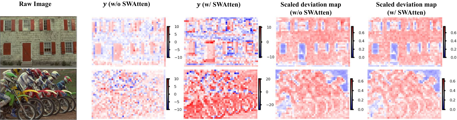
According to xie2021enhanced, the deviation between and with size can be used to analyze the information loss in the process of compression, we can formulate the mean absolute pixel deviation as:
| (6) | ||||
To compare the deviation among different models, it is unfair to directly compare the values because the and in different models have different ranges. Since the deviation is relative to , a scaling factor is introduced to define a scaled mean absolute pixel deviation to better evaluate the information loss. can be formulated as:
| (7) |
Fig. 5 shows the scaled deviation map and the channel with the largest entropy of of and in Kodak dataset by using the model with SWAtten or not. Note that the deviation map is in shape and each pixel is the mean of the absolute deviation along the channel dimension after scaling with . The for and can be reduced from 0.451 and 0.422 by using the model without SWAtten to 0.389 and 0.365 by using the model with SWAtten. It suggests that the model with SWAtten can have less information loss and get a higher quality decompressed image.
4 Experiments
4.1 Experimental Setup
4.1.1 Training Details
For training, we randomly choose 300k images of size larger than from ImageNet deng2009large, and randomly crop them with the size of during the training process. We adopt Adam kingma2014adam with a batch size 8 to optimize the network. The initial learning rate is set as . After 1.8M steps, the learning rate is reduced to for the last 0.2M steps.
The model is optimized by RD-formula as Equation 3. Two kinds of quality metrics, i.e., mean square error (MSE) and MS-SSIM, are used to represent the distortion . When the model is optimized by MSE, the belongs to . When the model is optimized by MS-SSIM, the belongs to .
For swin-transformer blocks, window sizes are set as 8 in the main path ( and ), and 4 in the hyper-prior path ( and ). The channel number of the latent is set as 320, while that of is set as 192, respectively. Other hyper-parameters in the entropy model follow the setting in minnen2020channel. We use RTX 3090 and Intel i9-10900K to complete the following experiments.
4.1.2 Evaluation
We test our method on three datasets, i.e., Kodak image set kodak with the image size of , old Tecnick test set22 2 https://sourceforge.net/projects/testimages/files/OLD/asuni2014testimages with the image size of , CLIC professional validation dataset33 3 http://clic.compression.cc/2021/tasks/index.htmlclic with 2k resolution. Both PSNR and MS-SSIM are used to measure the distortion, while bits per pixel (bpp) are used to evaluate bitrates.
4.1.3 Definition of Various Models
In the experiments, to explore the performance of our model with different complexities, we tested three different models (small, medium and large by setting different channel number in the middle layers). The location of is shown in Fig. 2. The number of slices of the entropy model for all models with attention modules is reduced to 5 from 10 which is a common setting in minnen2020channel. More details are reported in Supplementary.
4.2 Rate-Distortion Performance
We compare our large model with state-of-the-arts (SOTA) learned end-to-end image compression algorithms, including balle2018variational, cheng2020learned, xie2021enhanced, chen2022two, kim2022joint, he2022elic, and zou2022devil. The classical image compression codec, VVC vvc is also tested by using VTM12.1. The rate-distortion performance on Kodak dataset is shown in Fig. 7. Both PSNR and MS-SSIM are tested on Kodak to demonstrate the robustness of our method. Here, we convert MS-SSIM to for clearer comparison. As we can see, at the same bitrate, we can improve up to about 0.4dB PSNR and 0.5dB MS-SSIM compared with SOTA methods. The results of CLIC dataset and Tecnick dataset are shown in Fig. 9 and Fig. 9, respectively. We also achieve similar good results on these two datasets. These results suggest that our method is robust and can achieve SOTA performance based on all of the three datasets with different resolutions. To get quantitative results, we present the BD-rate bdrate computed from PSNR-BPP curves as the quantitative metric. The anchor RD-performance is set as the results of VVC on different datasets (BD-rate=0%). Our method outperforms VVC (VTM-12.1) by 12.30%, 13.71%, 11.85% in BD-rate on Kodak, Tecnick, and CLIC datasets, respectively. Table 1 shows partial results on Kodak. More comparisons are reported in Supplementary.
4.3 Ablation Studies
4.3.1 Comparison with Transformer-only/CNN-only based Models
In order to show the effectiveness of our proposed Transformer-CNN Mixture (TCM) blocks, we compare our medium model without SWAtten modules to the Transformer-only based model and CNN-only based model in zhu2022transformerbased. The results are shown in Fig. 10(a). “Conv_ChARM” and “SwinT_ChARM” are a CNN-only based model and a Transformer-only based model, respectively. They have similar architectures to our methods without SWAtten modules. The difference is that “SwinT_ChARM” uses Swin Transformer block, “Conv_ChARM” uses convolutional neural networks, and we use the proposed TCM block. By using the advantages both of transformer and CNN, the results show that our method surpasses the Transformer-only based model and CNN-only based model.
4.3.2 SWAtten Module
In Fig. 10(b), we compare the cases using SWAtten modules or not. It can be observed that SWAtten modules bring a significant gain in RD-performance. Meanwhile, by using the channel squeeze operation in SWAtten modules, we can get a comparable performance compared with the situation without using that operation while saving many parameters. Section 4.5 shows more information on the parameters efficiency gain of this operation.
4.4 Various Attention Modules
In Fig. 10(c), we compared our proposed SWAtten with the previous attention modules, including the non-local attention (NonlocalAtten) module liu2019non, the local attention (LocalAtten) module cheng2020learned, and the window-based attention (WAtten) module zou2022devil. Compared with these different attention modules, SWAtten gets the best RD-performance because it can capture non-local information while also paying enough attention to local information.
4.5 Complexity and Qualitative Results
We test the complexity and qualitative results of different methods based on Kodak. Two other SOTA works xie2021enhanced; zhu2022transformerbased, are also tested as Table 1 shows. The results of our method suggest that the efficiency and RD-performance of our method can outperform both of these two methods. Meanwhile, after using channel squeeze in SWAtten, we can save a lot of parameters and FLOPs, while we can get a comparable BD-rate. It also should be noted that all of our small, medium and large models can achieve SOTA RD-performance. Meanwhile, the performance can further improve as the complexity increases, which shows that our model has a lot of potentials.
| Methods |
|
|
|
|
| ||||||||||
|---|---|---|---|---|---|---|---|---|---|---|---|---|---|---|---|
| Xie et al. xie2021enhanced | 2346 | 5212 | 47.55 | 408.21 | -1.65 | ||||||||||
|
132 | 84 | 60.55 | 230.37 | -4.02 | ||||||||||
|
151 | 141 | 160.45 | 830.90 | -12.54 | ||||||||||
| Ours(Large) | 150 | 140 | 75.89 | 700.96 | -12.30 | ||||||||||
| Ours(Medium) | 130 | 122 | 58.72 | 415.20 | -9.65 | ||||||||||
| Ours(Small) | 109 | 102 | 44.96 | 211.54 | -7.39 |
4.6 Visualization
5 Conclusion
In this paper, we incorporate transformers and CNN to propose an efficient parallel transformer-CNN mixture block that utilizes the local modeling ability of CNN and the non-local modeling ability of transformers. Then, a new image compression architecture is designed based on the TCM block. Besides, we present a swin-transformer-based attention module to improve channel-wise entropy models. The results of experiments show that the image compression model with TCM blocks outperforms the CNN-only/Transformer-only based models under a suitable complexity. Furthermore, the performance of SWAtten surpasses previous attention modules designed for image compression. At last, our method achieves state-of-the-art on three different resolution datasets (i.e., Kodak, Tecnick, CLIC Professional Validation) and is superior to existing image compression methods.
6 Acknowledgment
This paper is supported by Japan Science and Technology Agency (JST), under Grant JPMJPR19M5; Japan Society for the Promotion of Science (JSPS), under Grant 21K17770; Kenjiro Takayanagi Foundation; the Foundation of Ando Laboratory; NICT, Grant Number 03801, Japan.
References
- (1) Nicola Asuni and Andrea Giachetti. Testimages: a large-scale archive for testing visual devices and basic image processing algorithms. In STAG, pages 63–70, 2014.
- (2) Johannes Ballé, Valero Laparra, and Eero P Simoncelli. End-to-end optimized image compression. In International Conference on Learning Representations, 2016.
- (3) Johannes Ballé, David Minnen, Saurabh Singh, Sung Jin Hwang, and Nick Johnston. Variational image compression with a scale hyperprior. In Proceedings of the International Conference on Learning Representations, 2018.
- (4) Gisle Bjontegaard. Calculation of average psnr differences between rd-curves. In VCEG-M33, 2001.
- (5) Fangdong Chen, Yumeng Xu, and Li Wang. Two-stage octave residual network for end-to-end image compression. In Proceedings of AAAI conference on artificial intelligence, 2022.
- (6) Zhengxue Cheng, Heming Sun, Masaru Takeuchi, and Jiro Katto. Learned image compression with discretized gaussian mixture likelihoods and attention modules. In Proceedings of the IEEE/CVF Conference on Computer Vision and Pattern Recognition, pages 7939–7948, 2020.
- (7) CLIC. Workshop and challenge on learned image compression. In Proceedings of the IEEE/CVF Conference on Computer Vision and Pattern Recognition, 2021.
- (8) Jia Deng. A large-scale hierarchical image database. Proceedings of IEEE/CVF conference on Computer Vision and Pattern Recognition, 2009.
- (9) Alexey Dosovitskiy, Lucas Beyer, Alexander Kolesnikov, Dirk Weissenborn, Xiaohua Zhai, Thomas Unterthiner, Mostafa Dehghani, Matthias Minderer, Georg Heigold, Sylvain Gelly, et al. An image is worth 16x16 words: Transformers for image recognition at scale. In International Conference on Learning Representations, 2020.
- (10) Haisheng Fu, Feng Liang, Jianping Lin, Bing Li, Mohammad Akbari, Jie Liang, Guohe Zhang, Dong Liu, Chengjie Tu, and Jingning Han. Learned image compression with discretized gaussian-laplacian-logistic mixture model and concatenated residual modules. arXiv preprint arXiv:2107.06463, 2021.
- (11) Google. Web picture format. 2010.
- (12) Zongyu Guo, Zhizheng Zhang, Runsen Feng, and Zhibo Chen. Causal contextual prediction for learned image compression. IEEE Transactions on Circuits and Systems for Video Technology, 32(4):2329–2341, 2021.
- (13) Dailan He, Ziming Yang, Weikun Peng, Rui Ma, Hongwei Qin, and Yan Wang. Elic: Efficient learned image compression with unevenly grouped space-channel contextual adaptive coding. In Proceedings of the IEEE/CVF Conference on Computer Vision and Pattern Recognition, 2022.
- (14) Dailan He, Yaoyan Zheng, Baocheng Sun, Yan Wang, and Hongwei Qin. Checkerboard context model for efficient learned image compression. In Proceedings of the IEEE/CVF Conference on Computer Vision and Pattern Recognition, pages 14771–14780, 2021.
- (15) Jun-Hyuk Kim, Byeongho Heo, and Jong-Seok Lee. Joint global and local hierarchical priors for learned image compression. In Proceedings of the IEEE/CVF Conference on Computer Vision and Pattern Recognition, pages 5992–6001, 2022.
- (16) Diederik P Kingma and Jimmy Ba. Adam: A method for stochastic optimization. arXiv preprint arXiv:1412.6980, 2014.
- (17) Eastman Kodak. Kodak lossless true color image suite (photocd pcd0992). 1993.
- (18) A Burakhan Koyuncu, Han Gao, and Eckehard Steinbach. Contextformer: A transformer with spatio-channel attention for context modeling in learned image compression. In European Conference on Computer Vision, 2022.
- (19) Jingyun Liang, Jiezhang Cao, Guolei Sun, Kai Zhang, Luc Van Gool, and Radu Timofte. Swinir: Image restoration using swin transformer. In Proceedings of the IEEE/CVF International Conference on Computer Vision, pages 1833–1844, 2021.
- (20) Fangzheng Lin, Heming Sun, Jinming Liu, and Jiro Katto. Multistage spatial context models for learned image compression. arXiv preprint arXiv:2302.09263, 2023.
- (21) Haojie Liu, Tong Chen, Peiyao Guo, Qiu Shen, Xun Cao, Yao Wang, and Zhan Ma. Non-local attention optimized deep image compression. arXiv preprint arXiv:1904.09757, 2019.
- (22) Ze Liu, Yutong Lin, Yue Cao, Han Hu, Yixuan Wei, Zheng Zhang, Stephen Lin, and Baining Guo. Swin transformer: Hierarchical vision transformer using shifted windows. In Proceedings of the IEEE/CVF International Conference on Computer Vision, pages 10012–10022, 2021.
- (23) Ming Lu, Peiyao Guo, Huiqing Shi, Chuntong Cao, and Zhan Ma. Transformer-based image compression. arXiv preprint arXiv:2111.06707, 2021.
- (24) Ao Luo, Heming Sun, Jinming Liu, and Jiro Katto. Memory-efficient learned image compression with pruned hyperprior module. In 2022 IEEE International Conference on Image Processing (ICIP), pages 3061–3065, 2022.
- (25) Wenjie Luo, Yujia Li, Raquel Urtasun, and Richard Zemel. Understanding the effective receptive field in deep convolutional neural networks. Advances in neural information processing systems, 29, 2016.
- (26) David Minnen, Johannes Ballé, and George D Toderici. Joint autoregressive and hierarchical priors for learned image compression. Advances in neural information processing systems, 31, 2018.
- (27) David Minnen and Saurabh Singh. Channel-wise autoregressive entropy models for learned image compression. In IEEE International Conference on Image Processing (ICIP), pages 3339–3343. IEEE, 2020.
- (28) Yichen Qian, Xiuyu Sun, Ming Lin, Zhiyu Tan, and Rong Jin. Entroformer: A transformer-based entropy model for learned image compression. In International Conference on Learning Representations, 2021.
- (29) Joint Video Experts Team. Vvc official test model vtm. 2021.
- (30) Hugo Touvron, Matthieu Cord, Matthijs Douze, Francisco Massa, Alexandre Sablayrolles, and Hervé Jégou. Training data-efficient image transformers & distillation through attention. In International Conference on Machine Learning, pages 10347–10357. PMLR, 2021.
- (31) Gregory K Wallace. The jpeg still picture compression standard. IEEE transactions on consumer electronics, 38(1):xviii–xxxiv, 1992.
- (32) Dezhao Wang, Wenhan Yang, Yueyu Hu, and Jiaying Liu. Neural data-dependent transform for learned image compression. In Proceedings of the IEEE/CVF Conference on Computer Vision and Pattern Recognition, pages 17379–17388, 2022.
- (33) Yaojun Wu, Xin Li, Zhizheng Zhang, Xin Jin, and Zhibo Chen. Learned block-based hybrid image compression. IEEE Transactions on Circuits and Systems for Video Technology, 2021.
- (34) Yueqi Xie, Ka Leong Cheng, and Qifeng Chen. Enhanced invertible encoding for learned image compression. In Proceedings of the 29th ACM International Conference on Multimedia, pages 162–170, 2021.
- (35) Kai Zhang, Yawei Li, Jingyun Liang, Jiezhang Cao, Yulun Zhang, Hao Tang, Radu Timofte, and Luc Van Gool. Practical blind denoising via swin-conv-unet and data synthesis. arXiv preprint arXiv:2203.13278, 2022.
- (36) Yinhao Zhu, Yang Yang, and Taco Cohen. Transformer-based transform coding. In International Conference on Learning Representations, 2022.
- (37) Renjie Zou, Chunfeng Song, and Zhaoxiang Zhang. The devil is in the details: Window-based attention for image compression. Proceedings of the IEEE/CVF conference on computer vision and pattern recognition, 2022.
Appendix A Classical Image Compression Standard Setting
A.1 VVC
We use VTM-12.1 which is built form the website44 4 https://vcgit.hhi.fraunhofer.de/jvet/VVCSoftware_VTM/-/releases/VTM-12.1 to achieve VVC. The script from CompressAI 55 5 https://github.com/InterDigitalInc/CompressAI/tree/master/compressai/utils/bench is utilized to evaluate model. The command is as the following:
A.2 WebP
We use the API of Pillow (PIL) to achieve WebP algorithm. The code is:
where quality is set as {5,10,15,20,25,30,35,40,45,50}.
| Methods | Dataset | BD-Rate |
| Cheng et al. cheng2020learned | Kodak 768x512 | 3.16 |
| Xie et al. xie2021enhanced | -1.65 | |
| Chen et al. chen2022two | -6.21 | |
| He et al. he2022elic | -7.49 | |
| Ours (Large) | -12.30 | |
| Ours (Medium) | -9.65 | |
| Ours (Small) | -7.39 | |
| Ballé et al. balle2018variational | Tecnick 1200x1200 | 30.66 |
| Xie et al. xie2021enhanced | -4.07 | |
| Kim et al. kim2022joint | 6.98 | |
| Ours (Large) | -13.71 | |
| Ours (Medium) | -11.29 | |
| Ours (Small) | -9.53 | |
| Cheng et al. cheng2020learned | CLIC-P val 2K | 6.77 |
| Xie et al. xie2021enhanced | -2.60 | |
| Chen et al. chen2022two | -7.15 | |
| Zou et al. zou2022devil | -3.68 | |
| Ours (Large) | -11.85 | |
| Ours (Medium) | -10.27 | |
| Ours (Small) | -8.94 | |
| VVC | - | 0 |
Appendix B Detailed Network Architecture
The architecture of the our method is shown in Fig. 11. The head dimensions of TCM blocks in and are set as {8, 16, 32, 32, 16, 8}, while the head dimensions of TCM blocks in and are set as 32. We set channel numbers of TCM blocks as 128/192/256 for Small/Medium/Large model. RBS and RBU have the same architectures as in cheng2020learned. The numbers of channels of the middle convolutional layers in RBS and RBU are 64/96/128 for our Small/Medium/Large model, while the number of last layer of RBS and RBU is 128/192/256. Here, to achieve the balance between running speed and RD-performance, we reduce the slices number in minnen2020channel from 10 to 5. Therefore, we have 5 Channel-Conditional Parameter Nets with SWAtten to get {} and {}. Also, we have 5 Latent Residual Prediction to get {}. All the restored slices are concatenated as which is sent to decoder to get a decompressed image.
Appendix C Comparison with Recent LIC Works
To get quantitative results, we present the BD-rate bdrate computed from PSNR-BPP curves as the quantitative metric. The anchor RD-performance is set as the results of VVC on different datasets (BD-rate=0%). The Table 2 shows the results. As results show, we outperform the previous works and achieve SOTA performance based on the three datasets with different resolutions.
Appendix D Ablation Studies on Various Entropy Estimation Models
To verify our TCM blocks can improve the overall RD-performance, in addition to test the model with the channel-wise entropy model in minnen2020channel, we also try the model using the spatial-wise entropy model in minnen2018joint. The results are shown in Fig. 12. We define the model where the main path uses TCM block as “TCMmain”. We compare the TCMmain model using spatial-wise entropy model with “SwinT-Hyperprior” model in zhu2022transformerbased and the model in cheng2020learned. All of these three methods use spatial-wise entropy models. The difference is that our model is based on TCM block, the model in cheng2020learned is based on CNN, and “SwinT-Hyperprior” is based on swin-transformer. As we can see, our method can get the best RD-performance. This suggests that the TCM blocks can significantly improve image compression, and are robust to different entropy models.
Appendix E Ablation Studies on the Numbers of Slices
The number of slices is an important hyper-parameter for channel-wise entropy model in minnen2020channel. A larger number leads to lower efficiency, while a lower number causes a worse RD-performance. To find a suitable number, we test some different number setting for our entropy model with the proposed SWAtten. The main path of the tested model is the same as the main path in minnen2020channel. The entropy model is also similar, the difference is that we add SWAtten. The results are shown in Fig. 13. As we can see, when is low, we get a bad RD-performance. With increasing, the performance is improved. But when , the improvement of the performance is not obvious, and even decreases. This indicates that 5 slices have been able to learn enough information in our model. Therefore, we set as 5 in our model to achieve the balance between running speed and RD-performance.
Appendix F Abaltion Studies on the Design of SWAtten
We test the SWAtten w/o CNN for attention map (green point) in Fig. 14. In addition, we also evaluate the case w/o the swin transformer (yellow point). From the results, we can see that using either of these two modules can bring about 0.1dB PSNR improvement with fewer bitrates.
Appendix G Visualization
We conducted a comparison between our TCM-based model and both a CNN-based cheng2020learned and Transformer-based zou2022devil model using the Kodak dataset’s and images. The results of this comparison are presented in Fig. 15. We focused our analysis on two local regions, and the differences between the three models are noticeable. In the upper local area of , our method effectively reconstructed some of the road sign details while making it easier to differentiate between the back fences. The pasted poster color is also clearer and not distorted. In contrast, our method generated fewer artifacts compared to the CNN-based/Transformer-based models when reconstructing the lower local region. For , our method generated the clearest sign in the left local region, and we achieved a clearer “E” letter than the other two methods in the right local region.
