Dynamic Subspace Estimation with Grassmannian Geodesics

We start with the following broad generative model for data arising from a time-varying subspace. At each time point $i$ we observe $\ell$ vectors from a time-varying subspace. Let $\bm{X}_{i}\in\mathbb{R}^{d\times\ell}$ for $i=1,2,\dots,T$ be data generated from a low-rank model with noise:

where $\bm{U}_{i}\in\mathbb{R}^{d\times k}$ is a matrix with orthonormal columns representing a point on the Grassmannian $\mathop{{}\mathcal{G}\left(k,d\right)}\nolimits$, the space of all rank-$k$ subspaces in $\mathbb{R}^{d}$; $\bm{G}_{i}\in\mathbb{R}^{k\times\ell}$ holds weight or loading vectors; and $\bm{N}_{i}\in\mathbb{R}^{d\times\ell}$ is an independent additive noise matrix. We observe $\bm{X}_{i}$ and our objective is to estimate a sequence of subspaces $\{\bm{U}_{i}\}_{i=1}^{T}$ that generates the observed samples. $\bm{U}_{i}$ for $i=1,\dots,T$. Note that while we use “time-varying” to describe this generative model, it can vary over any index, and the algorithms we consider are batch in the sense that they use all the data $\bm{X}_{i}$, $i=1,\dots,T$ for estimating $\bm{U}_{i}$, $i=1,\dots,T$.

If $\bm{U}_{i}=\bar{\bm{U}}$ is static for all $i=1,2,\dots,T$, and if $\bm{G}_{i}$ has zero-mean columns, then we could concatenate all $\bm{X}_{i}$ together and apply the SVD, which is well-known to recover a good approximation of $\bar{\bm{U}}$ as long as the number of samples $\ell T$ is large enough to overcome the noise. However, if $\bm{U}_{i}$ is varying for every $i$, one can immediately see that if $\ell<k$, estimating $\bm{U}_{i}$ is impossible without further assumptions. Even when $\ell\geq k$, in many applications it is natural to impose a relationship between the $\bm{U}_{i}$ subspace matrices over time, to guarantee regularity properties or known application constraints. Various constraints have been studied in the literature, such as a slowly rotating subspace, a subspace that is mostly static except for intermittent sudden changes, or a subspace that changes one dimension at a time (Narayanamurthy and Vaswani, 2018). Those models are all subsumed by the piecewise geodesic model for dynamic subspaces, illustrated in Figure 1. In this work, we focus on efficiently learning a single geodesic.

Classical literature on subspace tracking uses online approaches to estimate the time-varying subspaces (Yang, 1995; Chi et al., 2013; Allen-Zhu and Li, 2017; Balzano et al., 2018; Haghighatshoar and Caire, 2018; Narayanamurthy and Vaswani, 2018; Vaswani et al., 2018; Comon and Golub, 1990). Early theoretical results were limited to asymptotic convergence guarantees with static underlying subspaces. Among the more recent works, the PETRELS algorithm (Chi et al., 2013) portrays a recursive least squares approach and provides convergence theory that assumes that the subspace changes at a particular instant and then stays constant for sufficient time so that the change can be tracked (also called the piecewise constant model). Narayanamurthy and Vaswani, 2018 relax the assumption of constant subspace to a very slowly varying subspace between the change points. For a review of these methods, see Vaswani et al., 2018.

Dynamic subspace estimation has also been studied for the more general Grassmannian geodesic model that is the focus of this paper (Lake and Keenan, 1998; Fuhrmann, 1997; Srivastava and Klassen, 2004; Hong et al., 2016). Unlike the subspace tracking problem, these contributions focus on batch data settings with access to the whole dataset for estimation, which is the approach we take herein. For example, Lake and Keenan, 1998 formulate the subspace tracking for any given epoch in the generative geodesic model in the form of a likelihood function to maximize. The likelihood is nonconcave, but the authors provide an annealing approach to solve it, which will have very high computational burden for many modern high-dimensional and large-data applications. Fuhrmann, 1997 and Srivastava and Klassen, 2004 have also studied the generative geodesic model. The solution provided by Srivastava and Klassen, 2004 is not applicable to large-scale settings since it relies on a sampling based strategy like Markov chain Monte-Carlo (MCMC) and hence is computationally intensive. On the other hand, the solution provided by Fuhrmann, 1997 is computationally inexpensive, but it only handles one-dimensional subspaces ($k=1$). In summary, major weaknesses of the state-of-the-art methods include high computational costs, lack of theoretical guarantees, and/or need to tune hyperparameters. This paper approaches the problem using modern nonconvex optimization tools, alleviating these issues by devising an algorithm that is parameter free other than the subspace dimension, descends the loss function monotonically, and uses thin SVDs to solve the problem.

Let $\bm{Q}\triangleq[\bm{H}\ \bm{Y}]$ and $\bm{Z}_{i}\triangleq[\mathop{{}{\operator@font cos}\left(\bm{\Theta}t_{i}\right)}\nolimits;\,\mathop{{}{\operator@font sin}\left(\bm{\Theta}t_{i}\right)}\nolimits]$. Then we rewrite our model (2) as $\bm{U}_{i}=\bm{Q}\bm{Z}_{i}$. By constraining $\bm{Q}\in\mathcal{V}^{d\times 2k}$, we also satisfy the constraints of $\bm{H}$ and $\bm{Y}$ individually.

Following Breloy et al., 2021, we form a linear majorizer for our loss (5) at $\bm{Q}^{{\scriptscriptstyle(}n{\scriptscriptstyle)}}$ and minimize it with a Stiefel constraint simply by projecting its negative gradient onto the Stiefel manifold. The update is then given by

where $\bm{W}\bm{\Sigma}\bm{V}^{\top}$ is the SVD of $\sum_{i=1}^{T}\bm{X}_{i}\bm{X}_{i}^{\top}\bm{Q}^{{\scriptscriptstyle(}n{\scriptscriptstyle)}}\bm{Z}_{i}\bm{Z}_{i}^{\top}$. Further, using the simplification from (5) we have $\hat{\bm{G}}_{i}^{\top}=\bm{X}_{i}^{\top}\bm{U}_{i}^{{\scriptscriptstyle(}n{\scriptscriptstyle)}}=\bm{X}_{i}^{\top}\bm{Q}^{{\scriptscriptstyle(}n{\scriptscriptstyle)}}\bm{Z}_{i}$. Using this equality we can express the summation term in (6) in terms $\bm{X}_{i}$, $\hat{}\bm{G}$, and $\bm{\Theta}$ as follows

where we let $\hat{\bm{G}}_{i}^{\top}=\bm{X}_{i}^{\top}\bm{U}_{i}^{{\scriptscriptstyle(}n{\scriptscriptstyle)}}=\bm{X}_{i}^{\top}\bm{Q}^{{\scriptscriptstyle(}n{\scriptscriptstyle)}}\bm{Z}_{i}$. Although here we eliminated $\left\{\bm{G}_{i}\right\}_{i=1}^{T}$ from our loss (5), if we had not, this same update could be derived as a block coordinate update on $\bm{Q}$ and $\left\{\bm{G}_{i}\right\}_{i=1}^{T}$. See Appendix A.1 for more details.

The loss (5) for fixed $\bm{H}$ and $\bm{Y}$ is a smooth function of $\bm{\Theta}$ and can be effectively optimized via an iterative quadratic majorize-minimize scheme. Here we provide an overview of the method. Appendix A.2 provides a more complete derivation of the majorizer. First, we simplify the loss (5)

where defining $\mathop{{}{\operator@font arctan}}\nolimits\!2(y,x)$ as the angle of the point $(x,y)$ in the 2D plane counter-clockwise from the positive $x$-axis, the associated constants $r_{i,j},\phi_{i,j},b_{i,j}$ are defined as

This loss is separable for each diagonal element of $\bm{\Theta}$, so we find each $\hat{}\theta_{j}$ via a (1D) minimization. Let $\mathop{{}f_{i,j}\left(\theta_{j}\right)}\nolimits\triangleq-r_{i,j}\mathop{{}{\operator@font cos}\left(2\theta_{j}t_{i}-\phi_{i,j}\right)}\nolimits+b_{i,j}$. Then (cf. Funai et al., 2008) the following $\mathop{{}q_{i,j}}\nolimits$ defines a quadratic majorizer for $\mathop{{}f_{i,j}}\nolimits$ at $\theta_{j}$

where the derivative $\mathop{{}\dot{f}_{i,j}}\nolimits$ and curvature function $\mathop{{}w_{\mathop{{}f_{i,j}}\nolimits}}\nolimits$ are given by

Appendix A.2.2 gives a detailed construction of $\mathop{{}w_{\mathop{{}f_{i,j}}\nolimits}}\nolimits$.

Our majorize-minimize iterations for each diagonal element of $\bm{\Theta}$ are then given by

Conceptually, each MM update can be interpreted as a gradient descent step with a variable step size $s^{{\scriptscriptstyle(}n{\scriptscriptstyle)}}={1/(\sum_{i=1}^{T}\mathop{{}w_{\mathop{{}f_{i,j}}\nolimits}\left(\theta_{j}^{{\scriptscriptstyle(}n{\scriptscriptstyle)}}\right)}\nolimits)}$ that is guaranteed to not increase the loss even without any line search. Indeed, as both updates just outlined are known for their monotonicity properties, we have the following monotonicity result for our overall algorithm. Since the algorithm monotonically decreases the loss, which is bounded, this implies that the loss always converges. Empirically we see convergence to the planted subspace end points in the vast majority of experiments, but not in all. A more thorough investigation of the loss landscape and algorithmic convergence properties is of great interest for future work.

Proof: It suffices to show that each block coordinate update does not increase the loss. Both the $[\bm{H}\ \bm{Y}]$ block and $\bm{\Theta}$ block updates are instances of MM methods that guarantee this property. See, for example, Sun et al., 2017 Section II.C for a general treatment and Breloy et al., 2021 Section III.B for MM convergence with the nonconvex Stiefel constraint.

In the case of synthetic data, we are able to compare our estimated geodesic $\hat{\bm{U}}(t)$ against the true geodesic from which the data was generated. Our error metric is the square root of the average squared subspace error between corresponding points along the geodesic

In practice, we approximate the integral by sampling the geodesic at a large number of time points. The subspace error (15) takes a minimum value of 0 when $\mathrm{span}(\hat{\bm{U}})=\mathop{{}\mathrm{span}\left(\bm{U}\right)}\nolimits$ and a maximum value of 1 when $\mathrm{span}(\hat{\bm{U}})\perp\mathop{{}\mathrm{span}\left(\bm{U}\right)}\nolimits$. As such, the geodesic error (16) is similarly bounded. For all of our synthetic experiments, we generated data from our planted model (1). $\bm{\Theta}$ was constrained to generate distance-minimizing geodesics, i.e., $\left\|\bm{\Theta}\right\|_{2}<\nicefrac{{\pi}}{{2}}$. We drew $\bm{G}_{i}$ from a standard normal distribution. The noise $\bm{N}_{i}$ is additive white Gaussian noise (AWGN) with standard deviation $\sigma$. Unless otherwise noted, we initialized the proposed method with a random geodesic for all experiments. For the experiments in Figure 2 and Figure 3, we formed a coarse estimate of the starting and ending rank-$k$ subspaces, and computed a geodesic between these subspaces with (Absil et al., 2004, (19)) for initialization.

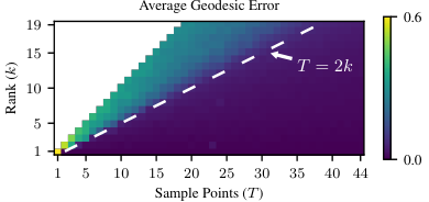
Figure 2 shows the average geodesic error when $\ell=1$, i.e., we receive one vector per $k$-dimensional subspace, as a function of both the true underlying rank ($k$) and the number of sample points ($T$). This plot shows that a phase transition occurs at $T=2k$, where if we have at least this many samples, the proposed method can recover the true geodesic with low error. At least $2k$ samples are necessary to compute the rank-$2k$ SVD, and this figure shows that $2k$ samples are also sufficient for computing the geodesic endpoints.

In Figure 3, we further investigate the effect of the number of samples on the average geodesic error. Because a rank-$k$ geodesic spans a space as large as $2k$, we have also shown for reference the subspace error of recovering a rank-$2k$ subspace with an SVD under two different distributions of loading vectors. The dashed lines show the subspace recovery error for data generated isotropically in a rank-$2k$ subspace with additive white Gaussian noise. The dotted lines show the subspace recovery error for data distributed on a geodesic in the rank-$2k$ subspace. Both SVD-based methods are only recovering a single rank-$2k$ subspace and not recovering a geodesic. Empirically, we can see that the sample complexity of the proposed geodesic model and method tracks well with rank-$2k$ SVD and outperforms SVD on geodesic data.

When the number of samples per time point ($\ell$) is less than $k$ the proposed method is still able to recover the true geodesic given that $T$ is large enough. When $\ell\geq k$, one could estimate the subspace at each time point by applying a rank-$k$ SVD at each time point. But, as shown in Figure 4, even when $\ell\geq k$, the proposed method recovers the subspaces at each time point with lower error for data generated from a geodesic.

Like a low-rank SVD approximation, our method requires choosing the rank $k$ before fitting. Figure 5 shows the loss as a function of assumed rank for data generated from a rank-1 geodesic (left) and rank-2 geodesic (right). Because a rank-$k$ geodesic spans a rank-$2k$ subspace, rank-$k$ and rank-$2k$ SVD results are shown for comparison. Rank-$2k$ SVD will always have a lower loss by definition. Similarly, the proposed model will always have a lower loss than the rank-$k$ SVD, since a rank-$k$ subspace is a special case of a rank-$k$ geodesic. Thus, we can lower-bound and upper-bound the loss of the proposed model on any data by a rank-$2k$ and rank-$k$ SVD respectively. Additionally, if the data has geodesic structure, then it is ordered. For comparison we also show the loss of the proposed method on data that was generated from a geodesic and then permuted. We see that when the assumed rank is equal to the true rank of the underlying geodesic, the proposed method produces a loss much closer to that of a rank-$2k$ SVD while the proposed method applied to permuted data produces a loss much closer to that of a rank-$k$ SVD. For permuted unordered data, the proposed model learns a geodesic with small values of $\bm{\Theta}$, approximating a static rank-$k$ subspace similar to a rank-$k$ SVD. For comparison, Figure 5 also shows the data error, which is the norm of the residual between the projected noisy data and the noiseless data. These plots show that rank-$2k$ SVD overfits the noise and has a higher error. The proposed method has a lower error than rank-$2k$ SVD for any assumed rank greater than or equal to the true rank on geodesic data.

Figure 6 compares the proposed geodesic algorithm to several online subspace tracking algorithms, including GROUSE (Balzano et al., 2010), Oja’s algorithm Oja, 1982, ISVD (Bunch and Nielsen, 1978), and PETRELS (Chi et al., 2013). We used $d=20,k=2,\ell=1$ and two noise levels. The proposed method consistently shows better performance (lower error) on geodesic data. See B.1 for detailed information. Appendix B.1 also contains additional synthetic experiments exploring a 2D loss surface and the effect of rank on the rate of convergence.

We show the effectiveness of the proposed method by applying it to (fully anonymized) dynamic functional MRI data collected with institutional review board approval. An effective data model for fMRI could be applied as part of an advanced image reconstruction algorithm, allowing for reduced scan times and higher temporal resolution without sacrificing image quality. We leave a full investigation of joint reconstruction and modeling as future work and, here, show only the viability of this model on fMRI data. In particular, we apply the proposed method on data collected with an oscillating steady state imaging (OSSI) (Guo and Noll, 2020) acquisition on a 3T GE MR750 scanner. Appendix B.2 and Guo and Noll, 2020 provide more details on acquisition and reconstruction parameters and example data. The OSSI acquisition rapidly cycles through 10 ($t_{\mathrm{fast}}$) different acquisition settings and then repeats this ($t_{\mathrm{slow}}$) for the duration of the scan. During the scan, subject breathing and scanner drift lead to slowly varying subspace changes that we hypothesized are suitable for a geodesic model. The scanner drift is approximately linear in time, so equally spaced $t_{i}$ values seems reasonable. The measurements are dynamic, high dimensional, and show redundant anatomical structure. As is common for image subspace models, we model a spatial patch of data.

Figure 7 shows the loss of applying the proposed method for a variety of ranks. Similar to Figure 5, we show a comparison to rank-$k$ and rank-$2k$ SVD and the proposed method on the data permuted. From this figure, we can see that the OSSI data appears to be well modeled by a rank 1 geodesic; the proposed method with rank 1 performs similarly to rank-$k$ SVD and permuting the data significantly increases the loss to that of rank-$k$ SVD.

In this section we apply the geodesic data model for a video denoising application. The video sequence used in this experiment is the first 260 frames of the Curtain video dataset (Li et al., 2004, Section V-A). The video sequence has variations due to a moving curtain and a person entering the scene at the end of the video. See more details and results for other videos in Appendix B.3.

We start by showing that the geodesic model is a good choice for this video data. Along similar lines as the fMRI data, we achieve this goal by computing loss (representation error) for approximating the video using rank-$k$ SVD, rank-$2k$ SVD, the proposed geodesic method, and applying the geodesic method after reordering/permuting the frames in video sequence. Again, the rationale behind permuting the frames is that if there is no temporal correlation in the frames then permuting the data would not have any negative impact on the loss. Figure 8 shows the training loss as a function of the rank $k$ and the PSNR of the denoised video as a function of added noise level. The training loss for the geodesic model lies in between $k$ and $2k$ cases, similar to the simulated data. More importantly, applying the geodesic model to permuted data degrades the loss, confirming that there is temporal correlation for the geodesic model to exploit. We add additive white Gaussian noise (AWGN) with different values of standard deviation $\sigma$ to the video sequence and applied rank-$k$ SVD, rank-$2k$ SVD, and the proposed geodesic subspace model to denoise the video sequence. The quality of the denoised image is measured using the peak signal to noise ratio (PSNR), defined as:

Figure 8 shows that rank-$2k$ SVD has the worst denoising performance (due to overfitting the very large amount of noise) while the proposed geodesic method has the best performance in the noisiest regime. For visual evidence, Figure 8(c) illustrates the denoising performance of rank-$k$ SVD and geodesic model for frame 125 in the sequence when noise of $\sigma=110$ is added. Again, similar to the simulated data, the superior denoising performance of geodesic model is quite evident.

References

- Absil et al., (2004) Absil, P.-A., Mahony, R., and Sepulchre, R. (2004). Riemannian geometry of grassmann manifolds with a view on algorithmic computation. Acta Applicandae Mathematica, 80(2):199–220.
- Allen-Zhu and Li, (2017) Allen-Zhu, Z. and Li, Y. (2017). Follow the compressed leader: faster online learning of eigenvectors and faster mmwu. In Proc. 34th Int. Conf. Mach. Learning, pages 116–125. JMLR. org.
- Balzano, (2022) Balzano, L. (2022). On the equivalence of oja’s algorithm and grouse. In International Conference on Artificial Intelligence and Statistics, pages 7014–7030. PMLR.
- Balzano et al., (2018) Balzano, L., Chi, Y., and Lu, Y. (2018). Streaming PCA and subspace tracking: The missing data case. Proc. of IEEE Special Issue on Rethinking PCA for Modern Datasets: Theory, Algorithms, and Applications.
- Balzano et al., (2010) Balzano, L., Nowak, R., and Recht, B. (2010). Online identification and tracking of subspaces from highly incomplete information. In 2010 48th Annual allerton conference on communication, control, and computing (Allerton), pages 704–711. IEEE.
- Boyd et al., (2010) Boyd, S., Parikh, N., Chu, E., Peleato, B., and Eckstein, J. (2010). Distributed optimization and statistical learning via the alternating direction method of multipliers. Found. & Trends in Machine Learning, 3(1):1–122.
- Breloy et al., (2021) Breloy, A., Kumar, S., Sun, Y., and Palomar, D. P. (2021). Majorization-minimization on the Stiefel manifold with application to robust sparse PCA. IEEE Trans. Sig. Proc., 69:1507–20.
- Bunch and Nielsen, (1978) Bunch, J. R. and Nielsen, C. P. (1978). Updating the singular value decomposition. Numerische Mathematik, 31(2):111–129.
- Chi et al., (2013) Chi, Y., Eldar, Y. C., and Calderbank, R. (2013). Petrels: Parallel subspace estimation and tracking by recursive least squares from partial observations. IEEE Trans. Signal Process., 61(23):5947–5959.
- Comon and Golub, (1990) Comon, P. and Golub, G. H. (1990). Tracking a few extreme singular values and vectors in signal processing. Proceedings of the IEEE, 78(8):1327–1343.
- Edelman et al., (1998) Edelman, A., Arias, T. A., and Smith, S. T. (1998). The geometry of algorithms with orthogonality constraints. SIAM J. Matrix. Anal. Appl., 20(2):303–53.
- Fessler, (2016) Fessler, J. A. (2016). Michigan image reconstruction toolbox (MIRT) for Matlab. Available from http://web.eecs.umich.edu/˜fessler.
- Fuhrmann, (1997) Fuhrmann, D. R. (1997). A geometric approach to subspace tracking. In Asilomar Conf. Signals, Syst. and Comput., volume 1, pages 783–787. IEEE.
- Funai et al., (2008) Funai, A. K., Fessler, J. A., Yeo, D. T. B., Olafsson, V. T., and Noll, D. C. (2008). Regularized field map estimation in MRI. IEEE Trans. Med. Imag., 27(10):1484–94.
- Golub and Pereyra, (2003) Golub, G. and Pereyra, V. (2003). Separable nonlinear least squares: the variable projection method and its applications. Inverse Prob., 19(2):R1–26.
- Guo and Noll, (2020) Guo, S. and Noll, D. C. (2020). Oscillating steady-state imaging (OSSI): A novel method for functional MRI. Mag. Res. Med., 84(2):698–712.
- Haghighatshoar and Caire, (2018) Haghighatshoar, S. and Caire, G. (2018). Low-complexity massive MIMO subspace estimation and tracking from low-dimensional projections. IEEE Trans. Signal Process., 66(7):1832–1844.
- Hong et al., (2016) Hong, Y., Kwitt, R., Singh, N., Vasconcelos, N., and Niethammer, M. (2016). Parametric regression on the grassmannian. IEEE Trans. Pattern Anal. Mach. Intell., 38(11):2284–2297.
- Huang et al., (2021) Huang, D., Niles-Weed, J., and Ward, R. (2021). Streaming k-pca: Efficient guarantees for oja’s algorithm, beyond rank-one updates. In Conference on Learning Theory, pages 2463–2498. PMLR.
- Lake and Keenan, (1998) Lake, D. E. and Keenan, D. (1998). Maximum likelihood estimation of geodesic subspace trajectories using approximate methods and stochastic optimization. In IEEE Signal Process. Workshop Statis. Signal and Array Process., pages 148–151. IEEE.
- Li et al., (2004) Li, L., Huang, W., Gu, I. Y.-H., and Tian, Q. (2004). Statistical modeling of complex backgrounds for foreground object detection. IEEE Trans. Image Process., 13(11):1459–1472.
- Narayanamurthy and Vaswani, (2018) Narayanamurthy, P. and Vaswani, N. (2018). Provable dynamic robust PCA or robust subspace tracking. IEEE Trans. Inform. Theory, 65(3):1547–1577.
- Oja, (1982) Oja, E. (1982). Simplified neuron model as a principal component analyzer. Journal of mathematical biology, 15(3):267–273.
- Otazo et al., (2015) Otazo, R., Candès, E., and Sodickson, D. K. (2015). Low-rank plus sparse matrix decomposition for accelerated dynamic MRI with separation of background and dynamic components. Magnetic Resonance in Medicine, 73(3):1125–1136.
- Srivastava and Klassen, (2004) Srivastava, A. and Klassen, E. (2004). Bayesian and geometric subspace tracking. Advances in Applied Probability, 36(1):43–56.
- Sun et al., (2017) Sun, Y., Babu, P., and Palomar, D. P. (2017). Majorization-minimization algorithms in signal processing, communications, and machine learning. IEEE Trans. Sig. Proc., 65(3):794–816.
- Uecker et al., (2014) Uecker, M., Lai, P., Murphy, M. J., Virtue, P., Elad, M., Pauly, J. M., Vasanawala, S. S., and Lustig, M. (2014). ESPIRiT-an eigenvalue approach to autocalibrating parallel MRI: Where SENSE meets GRAPPA. Mag. Res. Med., 71(3):990–1001.
- Vaswani et al., (2018) Vaswani, N., Bouwmans, T., Javed, S., and Narayanamurthy, P. (2018). Robust subspace learning: Robust pca, robust subspace tracking, and robust subspace recovery. IEEE Signal Process. Mag., 35(4):32–55.
- Yang, (1995) Yang, B. (1995). Projection approximation subspace tracking. IEEE Trans. Signal process., 43(1):95–107.
Supplementary Material for