Swampland criteria and constraints on inflation in a gravity theory
Abstract
In this paper, we worked in the framework of an inflationary theory, in the presence of a canonical scalar field. More specifically, the gravity. The values of the dimensionless parameters and are taken to be and . The motivation for that study was the striking similarities between the slow-roll parameters of the inflationary model used in this work and the ones obtained by the rescaled Einstein-Hilbert gravity inflation . We examined a variety of potentials to determine if they agree with the current Planck Constraints. In addition, we checked whether these models satisfy the Swampland Criteria and we specified the exact region of the parameter space that produces viable results for each model. As we mention in Section IV the inflationary theory used in this work can not produce a positive which implies that the stochastic gravitational wave background will not be detectable.
pacs
04.30.-w, 04.50.Kd, 11.25.-w, 98.80.-k, 98.80.CqI Introduction
In the upcoming years, various groundbreaking experiments are expected to take place. Their results could unveil aspects of the Cosmos that we ignored or could force us to review and amend current theories. Experiments like the LISA space mission Baker:2019nia; Smith:2019wny or the DECIGO Seto:2001qf; Kawamura:2020pcg are some of the most prominent. The importance of these next-generation observations comes from the fact that observing primordial gravitation waves (GW) is in reality proof that inflation occurred. This is possible only if the primordial spectrum of tensor perturbations is measured self consistency tests of inflation can be performed by comparing the spectrum of the tensor perturbations with one of the slow-roll parameters. Both of them will be introduced in Section III.
The majority of space interferometers can probe scales significantly smaller than Mpc, so they are in a regime, where Cosmic Microwave Background (CMB) scalar curvature perturbations are clearly non-linear. Excluding the Square Kilometer Array (SKA) Bull:2018lat and the NANOGrav collaboration Arzoumanian:2020vkk; Pol:2020igl, which could possibly test primordial GWs during the last stages of the radiation domination (RD) era, and the Planck collaboration Akrami:2018odb which tests large scales of very small frequencies, the remaining of the probes and observations could obtain information from GWs deeply during the RD era, when the universe is opaque and it’s impossible to gain information via photons observations. B-mode polarization modes are essential since they indicate that primordial tensor perturbations exist in large scales (multipoles of CMB that are approximately ) and there is a conversion of -modes to -modes, obviously at later times via direct gravitational lensing conversion, but this time for small angular scales in the CMB Denissenya:2018mqs.
The theory of inflation, which was developed by Alan Guth Guth:1980zm, is usually referred to as the rapidly accelerated era of the Universe, which emerged right after the quantum gravity era. Inflation provided the solution to some of the most puzzling Cosmological problems like the horizon problem, the flatness problem, the problem of initial energy, and the absence of primordial relics. The standard inflation model assumes the existence of a canonical scalar field named inflaton Linde:2007fr; Gorbunov:2011zzc; Lyth:1998xn; Martin:2018ycu. The idea of a canonical scalar field is an important key aspect of the most successful theories in particle physics and general in the field of high energy physics. Unfortunately, the only fundamental scalar field observed is the Higgs particle.
Since inflation took place right after the quantum gravity era it is rational to believe that some marks should be left in the effective Lagrangian during the inflation era and thus a modification of the Einstein-Hilbert action should possibly be applied with non-linear curvature corrections or with a general modification of the used action. Modified gravity theory has a lot of different forms and is considered as one of the most prominent candidate class of theories which contains higher order curvature corrections reviews1; reviews2; reviews3; reviews4; reviews5; reviews6. A large variety of works have unified the late-time accelerated era with the inflationary one, see fruitful works like Nojiri:2003ft and Refs. Nojiri:2007as; Nojiri:2007cq; Cognola:2007zu; Nojiri:2006gh; Appleby:2007vb; Elizalde:2010ts; Odintsov:2020nwm; Oikonomou:2020qah; Oikonomou:2020oex. One of the approaches that try to solve these problems is an gravity proposed by Harko et al. in Ref.Harko:2011kv. In this work, the gravity theory proposed by M.Gamonal in Ref.Gamonal:2020itt, slightly alternated, will be studied. Then the effective potentials studied in Ref.Oikonomou:2021zfl shall be considered for the Lagrangian and we will obtain further constraints for the introduced free parameters. In the next section, the second key aspect of the presented work will be introduced, which are the Swampland Criteria (SC). The final goal of this paper is to obtain the constraints for the introduced free parameters, imposed by SC and finally deduce if it is possible to have an agreement between them.
In this work the sections are structured as follows: In section II we present the Swampland Criteria for an inflationary theory, and in section III we specify the slow-roll conditions and observational parameters for the specific model that we studied. Section IV contains the Planck 2018 results as well as the methodology we followed in this paper. In section V we study several potentials and derive their constraints in light of the Planck results and the Swampland criteria. Finally, the conclusions and bibliography follow at the end of the article.
II Swampland Criteria for rescaled gravity
In this section, the SC for a gravity theory will be discussed. Their concept was first introduced in the Refs Vafa:2005ui; Ooguri:2006in and they have been studied in detail in Refs. Palti:2020qlc; Mizuno:2019bxy; Brandenberger:2020oav; Blumenhagen:2019vgj; Wang:2019eym; Benetti:2019smr; Palti:2019pca; Cai:2018ebs; Akrami:2018ylq; Mizuno:2019pcm; Aragam:2019khr; Brahma:2019mdd; Mukhopadhyay:2019cai; Yi:2018dhl; Gashti:2022hey; Brahma:2019kch; Haque:2019prw; Heckman:2019dsj; Acharya:2018deu; Elizalde:2018dvw; Cheong:2018udx; Heckman:2018mxl; Kinney:2018nny; Garg:2018reu; Lin:2018rnx; Park:2018fuj; Olguin-Tejo:2018pfq; Fukuda:2018haz; Wang:2018kly; Ooguri:2018wrx; Matsui:2018xwa; Obied:2018sgi; Agrawal:2018own; Murayama:2018lie; Marsh:2018kub; Storm:2020gtv; Trivedi:2020wxf; Sharma:2020wba; Odintsov:2020zkl; Mohammadi:2020twg; Trivedi:2020xlh; Oikonomou:2021zfl. These are criteria that are imposing conditions, which propose if an effective field theory is or not the correct description for quantum gravity for the high energy scales. So, an effective theory must satisfy the upcoming conditions:
- •
The Swampland distance conjecture, which limits the validity of an effective field theory by setting an upper bound for the maximum traversable range for a scalar field as following:
(1) - •
The de Sitter conjecture, which sets a lower bound for a scalar potential that is positive and its first derivative with respect to the scalar field. In reality, this states that it is impossible to create De Sitter vacua in string theory and reads as:
(2) We also have an interchangeable condition which includes the second derivative of the potential with respect to the field, which reads as follows:
(3)
note that the prime represents the differentiation with respect to the scalar field , and is the reduced Planck mass and denotes the value of the scalar field during the first horizon crossing. At this point is important to underline that we check which values of the free parameters of the potentials introduced in Ref.Akrami:2018odb should be satisfied so that the SC are fulfilled. The reader should keep in mind that if at least one of the conditions 1, 2 or 3 are satisfied the SC are met.
III gravity, slow-roll conditions and observational parameters
In this paper, it will not be provided an extensive presentation of the slow-roll parameters and the derivation of the observational indices since these have been presented exceptionally in Ref.Gamonal:2020itt. Therefore it would be beneficial to directly continue with the analysis of the slow-roll conditions and observational parameters for a gravity. Firstly let us introduce the definition of follow-momentum tensor :
| (4) |
The background metric is a flat Friedmann-Robertson-Walker (FRW) metric, which has the following form:
| (5) |
where corresponds to the scale factor. As it is mentioned in the introduction the simplest scenario for inflation assumes the existence of the inflaton . The slow roll conditions were introduced to ensure that the inflationary era lasted long enough to solve the problems presented in the introduction. The slow-roll conditions can be quantified thanks to the slow-roll parameters and in this paper, an extensive presentation of the slow-roll parameters and the derivation of the observational indices will not be provided since this has already been presented in Ref.Hwang:2005hb, so only the most relevant for this work will be provided:
| (6) |
| (7) |
At this point we have to turn our focus on the the definition of the parameters and , which are given as follows:
| (8) |
| (9) |
It essential for our analysis to introduce,
| (10) |
| (11) |
At this point, it is extremely important to avoid a very common confusion. For the classical Einstein-Hilbert action the equation (6) leads directly to the equation (8) and vice versa. But for a general gravity theory this is not the case even if it is obvious to find a correspondence between the gravity theory and the classical one which is obtained by the Einstein-Hilbert action. At this point, we have also to underline the connection between the SC provided by equation 1 and the provided by equation (8), for reads,
| (12) |
The reader could possibly assume the existence of a tension between the satisfaction of the slow-roll conditions imposed to the slow-roll parameter and the condition for the satisfaction of the SCs. This obstacle is possible to overcome if a vital detail is recalled. The slow-roll indices are described by the conditions and and not by the conditions and . This is an important detail, which should be taken into consideration to avoid any confusion. To make these results crystal-clear we need to introduce the action, derive the equations of motion (EoM) and a rescaled Klein-Gordon (KG) equation. The general formulation of the EoM for an gravity theory is presented in the Ref.Gamonal:2020itt and since this work is limited in a it is beneficial the action to be directly provided. So, for , we have that:
| (13) |
so we can arrive at the equations of motion which according to the Ref.Gamonal:2020itt read:
| (14) |
The action in Eq. (13) may be the result of some higher order curvature effects at leading order during the inflationary era. For example Oikonomou:2020oex,
| (15) |
In the large curvature limit, the exponential term of Eq. (15) at leading order yields,
| (16) |
hence, the effective action during inflation contains terms of the Ricci scalar as follows,
| (17) |
where . So after the analysis we arrive at the following equations:
| (18) |
| (19) |
| (20) |
Finally the rescaled KG equation can be obtained, which according to Ref.Gamonal:2020itt reads as:
| (21) |
It should be mentioned that all the previous results reproduce the well-know results for the classical Einstein-Hilbert action by simply setting . At this point the spectral indices and their connection to the slow-roll parameters should be introduced, which according to the Ref.Gamonal:2020itt read as:
| (22) |
| (23) |
| (24) |
It should be mentioned, that up to this date there is no value for since the B-mode polarization for GW have not been observed. Recalling the definition of the by equation (6) for the model one can obtain:
| (25) |
The slow-roll parameters are formulated in such a way that we are able to quantify directly the required conditions to impose slow-roll conditions. For we demand that . Therefore the condition is:
| (26) |
so is now approximately equal to,
| (27) |
The KG becomes:
Following the methodology introduced in the Ref.Gamonal:2020itt, we can arrive at the derivation of the the observational indices with respect to the potential and the free parameters and introduced by our gravity model. We obtain the final expression for by substituting from equation (28) and from equation (29) in equation (27). So the primordial tilt reads as:
| (30) |
| (31) |
| (32) |
where
| (33) |
and
| (34) |
Here we come to an interesting realization, the slow roll indices and by extension , and depend only on the value of , which as we will soon see holds true for the e-folds number too. For that reason it is convenient to use in order to simplify the analysis and the rather complicated expressions that we will come across in this work.
IV Planck 2018 results and methodology presentation
The goal of this section is to present the methodology that will be followed in this work. Firstly the value of the inflaton at the end of inflation, is obtained by using the equation . At this point, the definition of the e-folding number should be recalled , so after some simple calculations we arrive at:
| (35) |
where . So, after calculating the number of e-folds, the can be obtained, which is essential to calculate since , and are calculated for . Then using the equations (30), (31) and (32) the observational indices are obtained as a function of , and possibly the free parameters the introduced potential has. It should be underlined that only two free parameters should be left in the final obtained results for the spectral indices so if there are more than three left the e-folding number will be eliminated by setting . Then, the remaining parameters are constraint using the Planck 2018 results from Ref.Akrami:2018odb. Namely,
| (36) |
We should mention that the parameter can only take positive values because a negative would result in a negative as can be seen in the expressions (32) and (33). Therefore, in this theory can only take negative values, which means that the primordial gravitational waves produced will not be detectable by any of the upcoming gravitational wave experiments.
At this point we turn our focus on the on the SC. By using the equations (1), (2) and (3) we are able to impose new constraints on the introduced free parameters and then compare with the ones we found on the first part of our analysis and finally deduce if it possible that SC and inflationary constraints are satisfied at the same time for the model we are studying.
V Derivation of the constraints on the inflationary models and SC.
V.1 Power law potentials
Let us start with the study of the general family of the power laws potentials. In general it can be written:
| (37) |
where has mass dimensions. Since the methodology used was presented in detail in Section IV the obtained results can be directly presented. The slow roll parameters for read:
| (38) |
| (39) |
At this point we can proceed for and arrive at the calculation of :
| (40) |
So, we are now able to derive the spectral indices for :
| (41) |
| (42) |
This is the most important part of the presented work since there are many ways to obtain the required bounds for the free parameters. It was chosen to eliminate since , was setted and and when it was necessary to end up with only 2 parameters free we set .
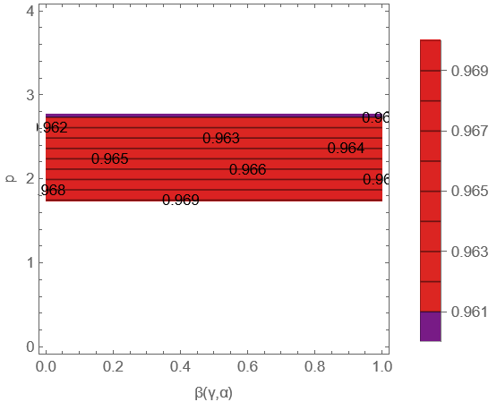
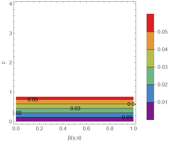
Using the Plank Constraints (36) we derived the constraints for the parameter of the model. In specific, the relation (41) for the scalar spectral index results in the following inequality,
| (43) |
while from (42) we calculate the inequality,
| (44) |
As can be seen, the two inequalities are incompatible, so the model is not viable.
Let us proceed to the calculation of the constraints that emerged from the SC. Using the equations (1), (2) and (3) and setting and we arrive at:
| (45) |
| (46) |
| (47) |
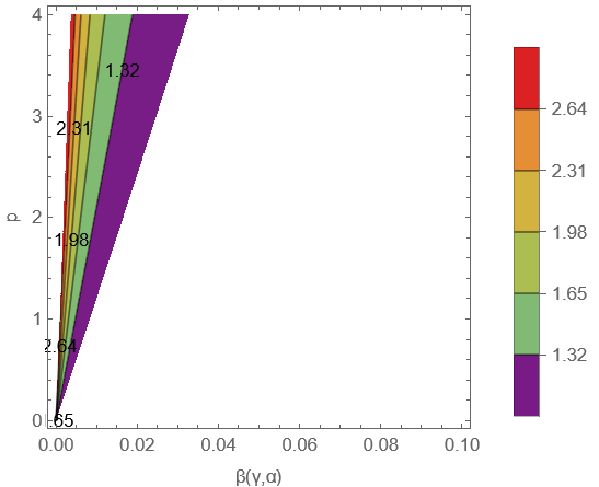
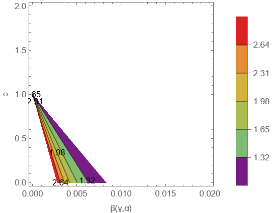
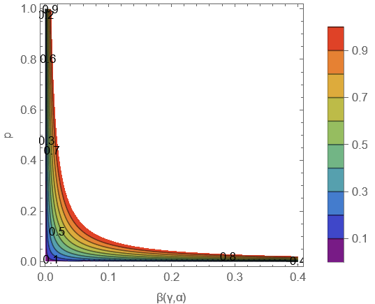
Using the (1) we calculate as well as,
| (48) |
For (2) to be satisfied,
| (49) |
Considering (3), we calculate the,
| (50) |
Taking the equations (45), (46) and (47) we will arrive at the figures Fig.2 and Fig.3, which prove the existence of a large variety of different values of the introduced free parameters that satisfy the SC. Since the primary goal was to obtain a result combining the two different sets of constraints and in this case this is impossible since the inflationary ones fail and thus no further progress can be achieved. Note that it is known that the Power Law models are fragile to be non-viable for the classic Einstein-Hilbert action and as it is proven in Oikonomou:2021zfl this is the situation even for a gravity approach. So, we decided to present extensively the results in between before we arrive at the final form of the observational indices. We will not insist on presenting extensively the results in between since the methodology we used is precisely given in Section IV.
V.2 D-Brane p=4
Lets us proceed by working on the D-Brane model Akrami:2018odb:
| (51) |
where has dimensions of mass [m] and is constructed in such a way it is dimensionless. Since the methodology used was presented in detail in Section IV we can directly proceed with the obtained results.
| (52) |
So using the methodology presented in Section IV and setting we arrived at:
| (53) |
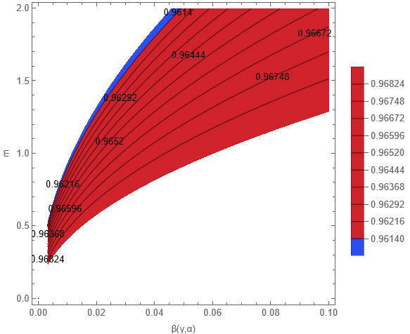
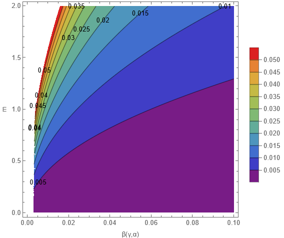
Using the above equations the demanded plots can be obtained to obtain the constraints, which are presented in Fig.4 and it makes obvious that there is indeed an area that constraints the free parameters in such a way that the observational conditions are met. Using (36) for we found that,
| (54) |
As for the tensor-to-scalar ratio, from (36) it follows that,
| (55) |
| (56) |
Thus, the model can be considered viable.
Let us proceed to the calculation of the constraints that emerged from the SC. Using the equations (1), (2) and (3) and setting and we arrive at:
| (57) |
| (58) |
| (59) |
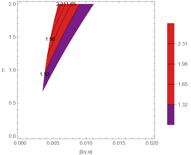
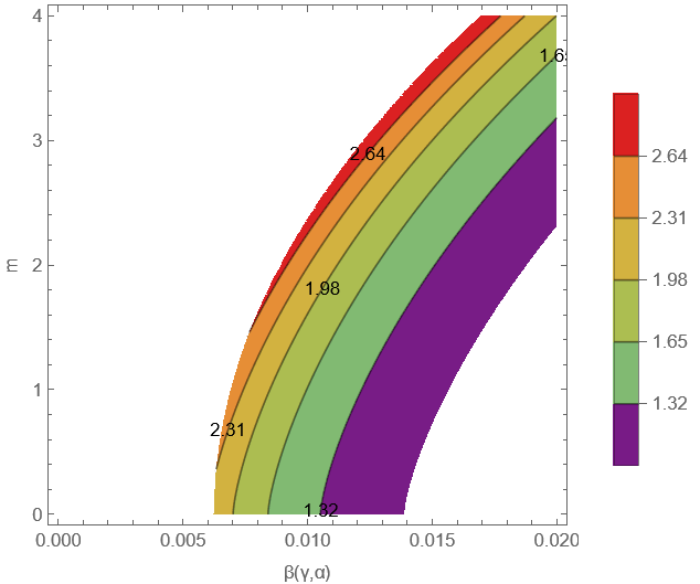
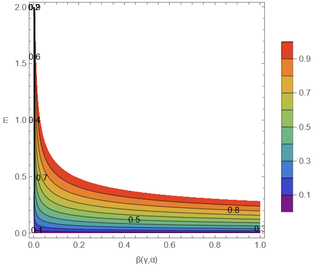
For the first SC (1) we calculate,
| (60) | ||||
For the (2) to be satisfied,
| (61) |
Considering the (3), we calculate the
| (62) |
V.3 E model
In this subsection, we proceed with the analysis of rather interesting potential, the E model for , which reads as:
| (63) |
where has mass dimensions and has no dimensions, in general, we are using the free parameters in such a way they are usually dimensionless because it is just slightly easier to work with. Flowing the methodology presented in section IV we derive the , which reads as:
| (64) |
So using that , the methodology presented in Section IV and setting we arrived at:
| (65) |
and
| (66) |
Using the above equations we can arrive at the demanded plots to obtain the constraints, which are presented in Fig.8 and it makes obvious that there is indeed an area that constraints the free parameters in such a way that the observational conditions are met. Using the Plank Constraints (36) we derived the constraints for the parameters and of the model. In specific, the relation (65) for the scalar spectral index results in the following inequality,
| (67) |
while from (42) we calculate the inequality,
| (68) |
As a result, we end up with,
| (69) |
so the model is viable.
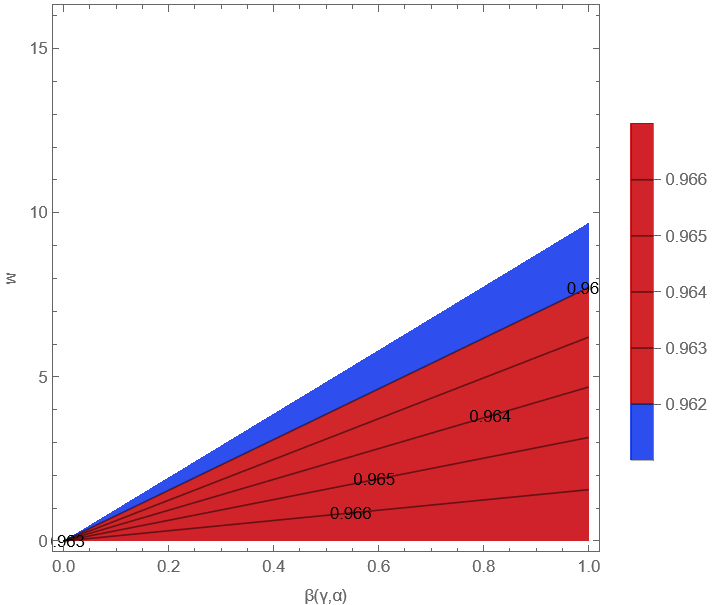
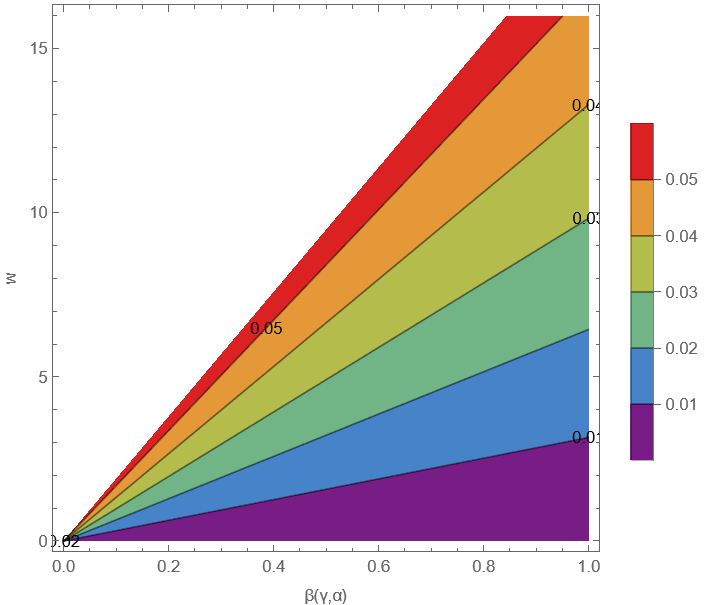
Let us proceed with the derivation of the constraints emerging from the SC. Using the equations (1), (2) and (3) and setting and we arrive at:
| (70) |
| (71) |
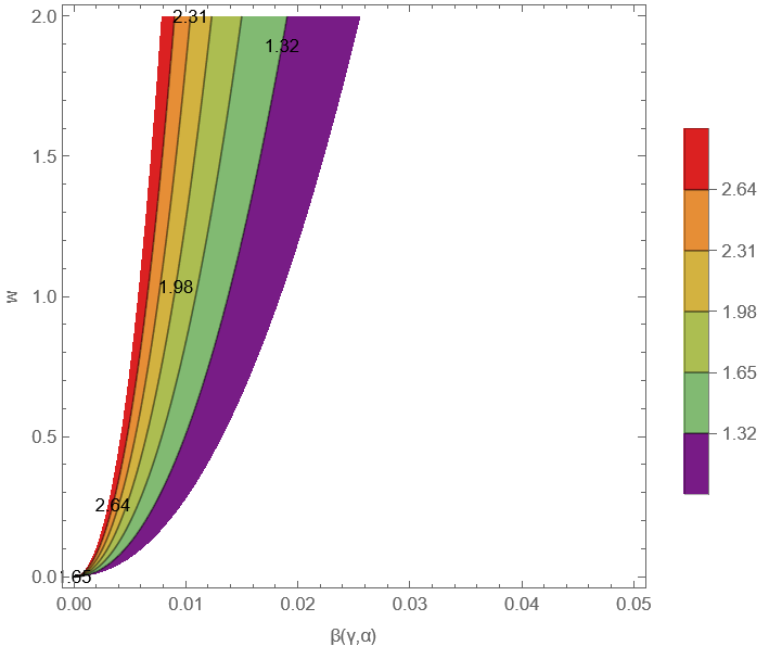
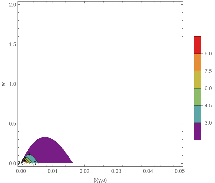
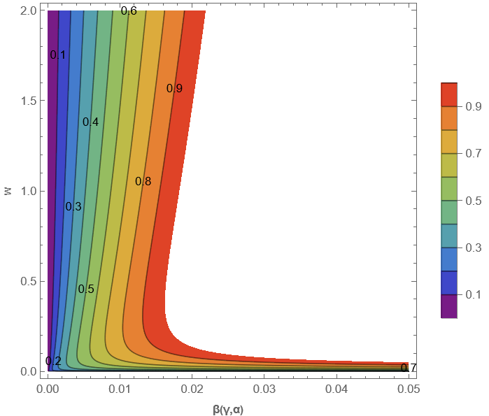
For (1) we get,
| (73) |
For the de Sitter conjecture to be satisfied, we derived the precise forms of the constraints for SC and conclude at,
| (74) |
Afterwards, we used the third SC and obtained the following inequalities,
| (75) | ||||
for , while for we obtained,
| (76) | ||||
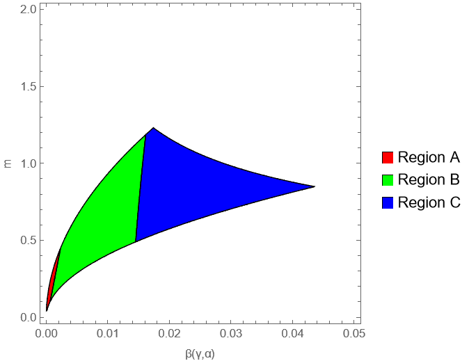
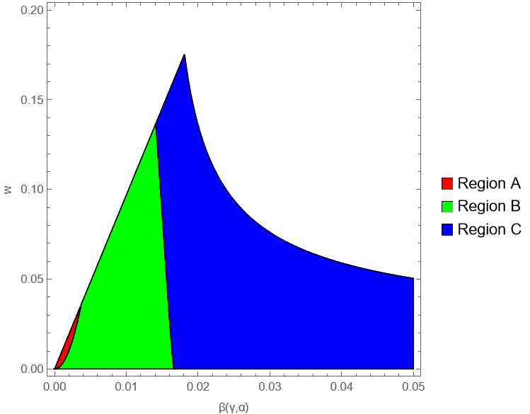
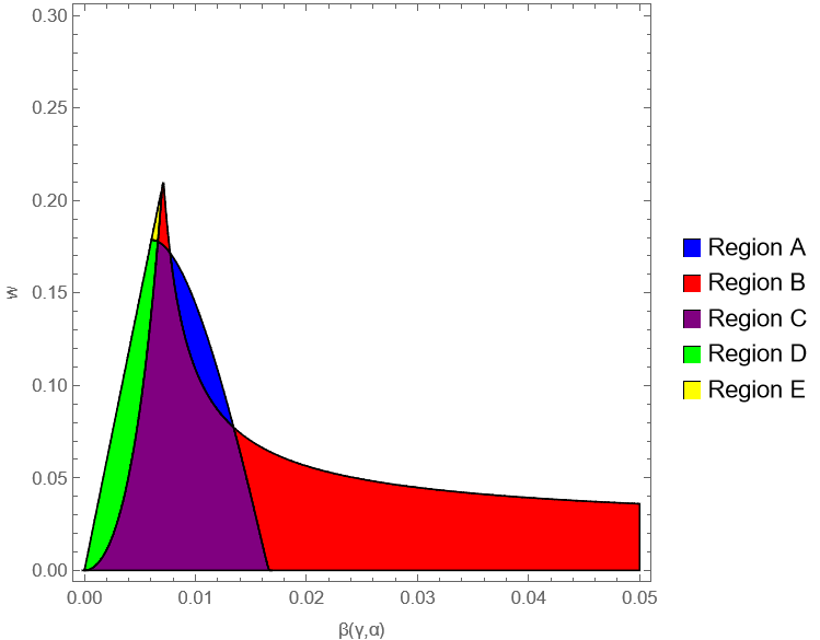
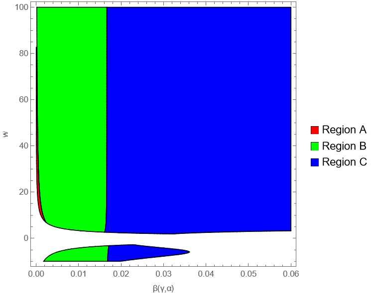
We present all the mentioned results in FIG. 11. We note that Region C of FIG. 11. extents to which contains GR, for and
V.4 T-Model(m=1) Model
We proceed this work with the T-Model (m=1):
| (77) |
where has dimension mass dimension, so and has no dimensions following the general philosophy to work with dimensionless parameters. By following the methodology provided in IV we find :
| (78) |
Following the methodology presented in Section IV and setting we arrived at:
| (79) |
and
| (80) |
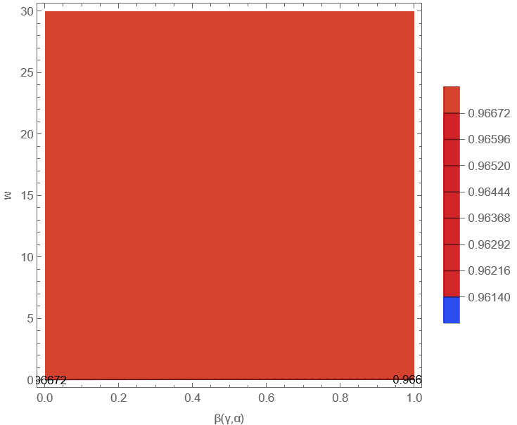
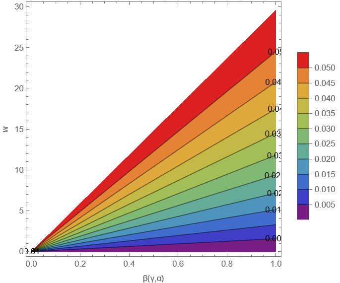
Using the above equations the demanded plots can be found to obtain the constraints, which are presented in the FIG.12 and it makes obvious that there is indeed an area that constraints the free parameters in such a way that the observational conditions are met. Using (36) and combine them with (79) and (80) one can compute the inequality,
| (81) |
which satisfy both and indices, so the model is viable.
Let us proceed with the derivation of the constraints emerging from the SC. Using the equations (1), (2) and (3) and setting and we arrive at:
| (82) |
| (83) |
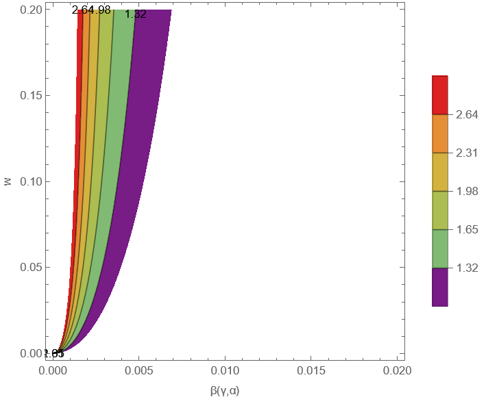
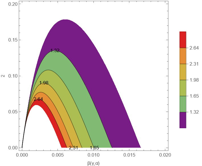
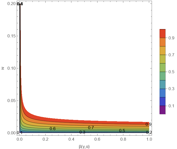
Though simplifying the SC inequalities analytically is challenging we can use numerical methods to get the approximate form of those inequalities in the interval Eventually, we calculate that for (1),
| (85) | ||||
As for (2) we obtain,
| (86) |
Finally, for (3) we calculate,
| (87) | ||||
It should be noted that the two above approximation fail very close to .
We present the combination of the Planck constraints and the Swampland Criteria in FIG. 15, we should mention that Region B of FIG. 15. extents to which contains GR, for and .
V.5 Modular Potential
In this case, we are going to study the following potential:
| (88) |
where has dimensions of mass so , is dimensionless and has the following dimensions . By following the methodology provided in IV we find :
| (89) |
So using the methodology presented in Section IV and setting we arrived at:
| (90) |
and
| (91) |
Using the above equations the demanded plots can be found to obtain the constraints, which are presented in the Fig.16 and it makes obvious that there is indeed an area that constraints the free parameters in such a way that the observational conditions are met. Taking the Plank Constraints (36) into account, and put them all together, we calculate
| (92) |
for and
| (93) |
for r. As a result, combining (92) and (93) both, it can be seen that for
| (94) |
the model is viable.
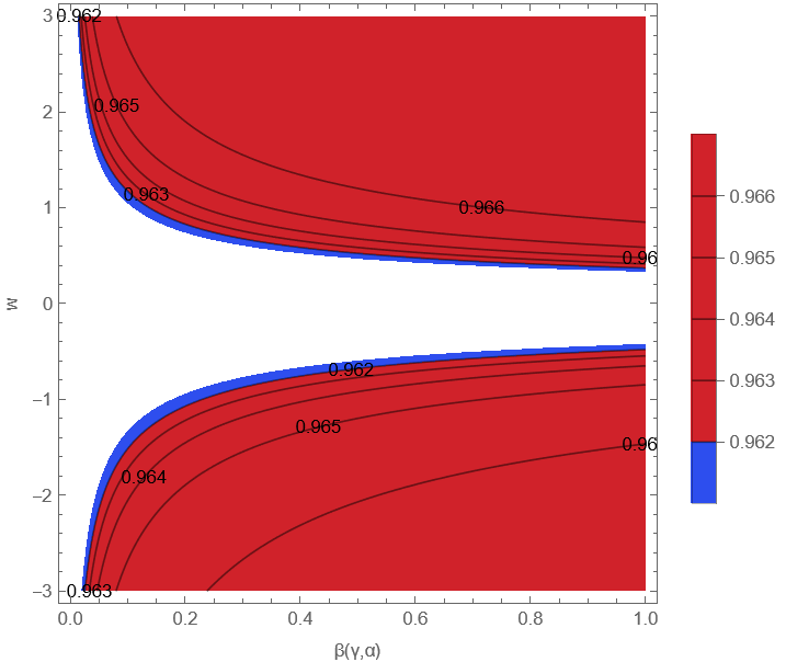
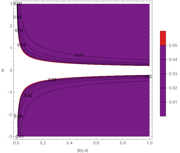
Let us proceed with the derivation of the constraints emerging from the SC. Using the equations (1), (2) and (3) and setting and we arrive at:
| (95) |
| (96) |
| (97) |
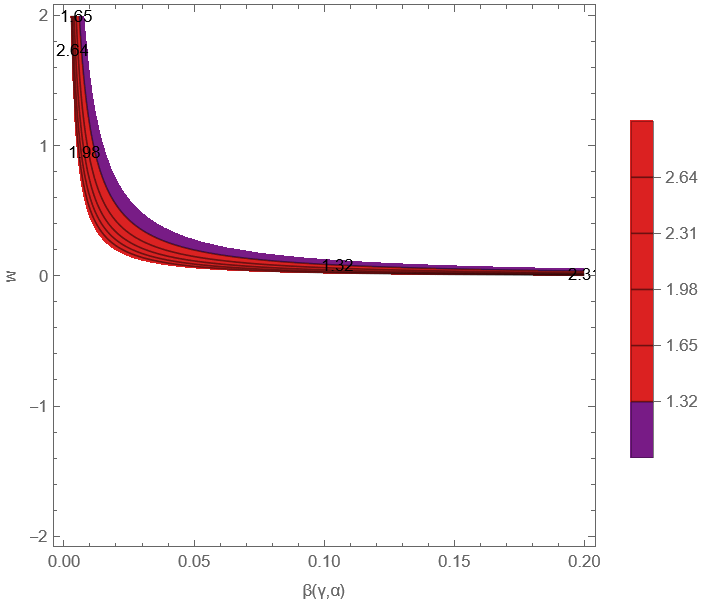
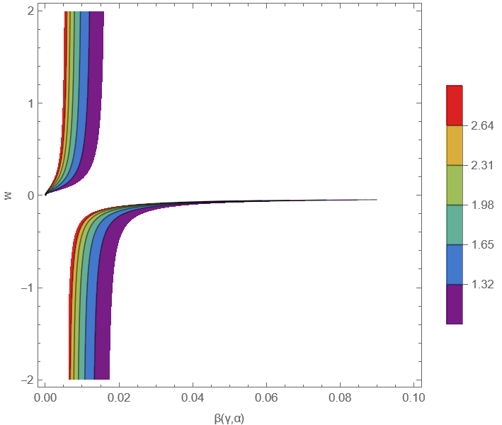
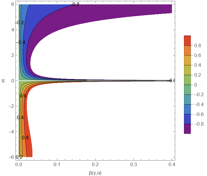
It is apparent that the expression (95) is very complicated. Therefore, the inequality of the first SC (1) cannot be simplified. However, the combination of (2) and (96) can be simplified further,
| (98) |
The combination of the Planck constraints and the Swampland Criteria is presented in FIG. 15, we should mention that Region C of FIG. 15. extents to which contains GR, for and .
VI Conclusions
In this work, we considered the gravity with a canonical minimally coupled scalar field as a model for inflation, with and . The main motivation behind this study was that the mentioned gravity yields similar relations for the slow-roll indices as a rescaled Einstein-Hilbert gravity. As we demonstrated, not all potentials generate viable results, more specifically, the Power law potentials proved to be non-viable, as the tensor-to-scalar ratio and the scalar spectral index are not compatible with the Planck Constraints in the same region of the parameter space. However, the rest of the studied models are compatible with both the latest Planck data (2018) and the Swampland Criteria. Using both analytical and numerical tools we were able to specify the region of the parameter space where both the Planck Constraints and the SC are satisfied and we presented the relevant region plots. Unfortunately, because must be positive, the tensor spectral index can only be negative, which means that the primordial gravitational waves produced will not be observed by any of the next-generation gravitational wave detectors. An important finding of this work is the simultaneous satisfaction of the Swampland Criteria and the Planck constraints in the GR limit. In future work, we would like to investigate the non-minimally coupled case, as a further generalization of this work.
References
- (1) J. Baker, J. Bellovary, P. L. Bender, E. Berti, R. Caldwell, J. Camp, J. W. Conklin, N. Cornish, C. Cutler and R. DeRosa, et al. [arXiv:1907.06482 [astro-ph.IM]].
- (2) T. L. Smith and R. Caldwell, Phys. Rev. D 100 (2019) no.10, 104055 doi:10.1103/PhysRevD.100.104055 [arXiv:1908.00546 [astro-ph.CO]]. ‘
- (3) N. Seto, S. Kawamura and T. Nakamura, Phys. Rev. Lett. 87 (2001), 221103 doi:10.1103/PhysRevLett.87.221103 [arXiv:astro-ph/0108011 [astro-ph]].
- (4) S. Kawamura, M. Ando, N. Seto, S. Sato, M. Musha, I. Kawano, J. Yokoyama, T. Tanaka, K. Ioka and T. Akutsu, et al. [arXiv:2006.13545 [gr-qc]].
- (5) T. Harko, F. S. N. Lobo, S. Nojiri and S. D. Odintsov, Phys. Rev. D 84 (2011), 024020 doi:10.1103/PhysRevD.84.024020 [arXiv:1104.2669 [gr-qc]].
- (6) M. Gamonal, Phys. Dark Univ. 31 (2021), 100768 doi:10.1016/j.dark.2020.100768 [arXiv:2010.03861 [gr-qc]].
- (7) A. Weltman, P. Bull, S. Camera, K. Kelley, H. Padmanabhan, J. Pritchard, A. Raccanelli, S. Riemer-Sørensen, L. Shao and S. Andrianomena, et al. Publ. Astron. Soc. Austral. 37 (2020), e002 doi:10.1017/pasa.2019.42 [arXiv:1810.02680 [astro-ph.CO]].
- (8) Z. Arzoumanian et al. [NANOGrav], Astrophys. J. Lett. 905 (2020) no.2, L34 doi:10.3847/2041-8213/abd401 [arXiv:2009.04496 [astro-ph.HE]].
- (9) N. S. Pol et al. [NANOGrav], [arXiv:2010.11950 [astro-ph.HE]].
- (10) Y. Akrami et al. [Planck Collaboration], arXiv:1807.06211 [astro-ph.CO].
- (11) M. Denissenya and E. V. Linder, JCAP 11 (2018), 010 doi:10.1088/1475-7516/2018/11/010 [arXiv:1808.00013 [astro-ph.CO]].
- (12) A. D. Linde, Lect. Notes Phys. 738 (2008) 1 doi:10.1007/978-3-540-74353-8_1 [arXiv:0705.0164 [hep-th]].
- (13) D. S. Gorbunov and V. A. Rubakov,“Introduction to the theory of the early universe: Cosmological perturbations and inflationary theory,” Hackensack, USA: World Scientific (2011) 489 p
- (14) D. H. Lyth and A. Riotto, Phys. Rept. 314 (1999) 1 doi:10.1016/S0370-1573(98)00128-8 [hep-ph/9807278].
- (15) J. Martin, arXiv:1807.11075 [astro-ph.CO].
- (16) S. Nojiri, S. D. Odintsov and V. K. Oikonomou, Phys. Rept. 692 (2017) 1 doi:10.1016/j.physrep.2017.06.001 [arXiv:1705.11098 [gr-qc]].
- (17) S. Nojiri, S.D. Odintsov, Phys. Rept. 505, 59 (2011);
- (18) S. Nojiri, S.D. Odintsov, eConf C0602061, 06 (2006) [Int. J. Geom. Meth. Mod. Phys. 4, 115 (2007)]. [arXiv:hep-th/0601213];
- (19) S. Capozziello, M. De Laurentis, Phys. Rept. 509, 167 (2011) [arXiv:1108.6266 [gr-qc]]. V. Faraoni and S. Capozziello, Fundam. Theor. Phys. 170 (2010). doi:10.1007/978-94-007-0165-6
- (20) A. de la Cruz-Dombriz and D. Saez-Gomez, Entropy 14 (2012) 1717 doi:10.3390/e14091717 [arXiv:1207.2663 [gr-qc]].
- (21) G. J. Olmo, Int. J. Mod. Phys. D 20 (2011) 413 doi:10.1142/S0218271811018925 [arXiv:1101.3864 [gr-qc]].
- (22) S. Nojiri and S. D. Odintsov, Phys. Rev. D 68 (2003) 123512 doi:10.1103/PhysRevD.68.123512 [hep-th/0307288].
- (23) S. Nojiri and S. D. Odintsov, Phys. Lett. B 657 (2007) 238 doi:10.1016/j.physletb.2007.10.027 [arXiv:0707.1941 [hep-th]].
- (24) S. Nojiri and S. D. Odintsov, Phys. Rev. D 77 (2008) 026007 doi:10.1103/PhysRevD.77.026007 [arXiv:0710.1738 [hep-th]].
- (25) G. Cognola, E. Elizalde, S. Nojiri, S. D. Odintsov, L. Sebastiani and S. Zerbini, Phys. Rev. D 77 (2008) 046009 doi:10.1103/PhysRevD.77.046009 [arXiv:0712.4017 [hep-th]].
- (26) S. Nojiri and S. D. Odintsov, Phys. Rev. D 74 (2006) 086005 doi:10.1103/PhysRevD.74.086005 [hep-th/0608008].
- (27) S. A. Appleby and R. A. Battye, Phys. Lett. B 654 (2007) 7 doi:10.1016/j.physletb.2007.08.037 [arXiv:0705.3199 [astro-ph]].
- (28) E. Elizalde, S. Nojiri, S. D. Odintsov, L. Sebastiani and S. Zerbini, Phys. Rev. D 83 (2011) 086006 doi:10.1103/PhysRevD.83.086006 [arXiv:1012.2280 [hep-th]].
- (29) S. D. Odintsov and V. K. Oikonomou, arXiv:2001.06830 [gr-qc].
- (30) V. K. Oikonomou, Phys. Rev. D 103 (2021) no.4, 044036 doi:10.1103/PhysRevD.103.044036 [arXiv:2012.00586 [astro-ph.CO]].
- (31) V. K. Oikonomou, [arXiv:2012.01312 [gr-qc]].
- (32) H. Ooguri and C. Vafa, Nucl. Phys. B 766 (2007) 21 doi:10.1016/j.nuclphysb.2006.10.033 [hep-th/0605264].
- (33) S. Mizuno, S. Mukohyama, S. Pi and Y. L. Zhang, Phys. Rev. D 102 (2020) no.2, 021301 doi:10.1103/PhysRevD.102.021301 [arXiv:1910.02979 [astro-ph.CO]].
- (34) R. Brandenberger, V. Kamali and R. O. Ramos, arXiv:2002.04925 [hep-th].
- (35) R. Blumenhagen, M. Brinkmann and A. Makridou, JHEP 2002 (2020) 064 [JHEP 2020 (2020) 064] doi:10.1007/JHEP02(2020)064 [arXiv:1910.10185 [hep-th]].
- (36) Z. Wang, R. Brandenberger and L. Heisenberg, arXiv:1907.08943 [hep-th].
- (37) M. Benetti, S. Capozziello and L. L. Graef, Phys. Rev. D 100 (2019) no.8, 084013 doi:10.1103/PhysRevD.100.084013 [arXiv:1905.05654 [gr-qc]].
- (38) E. Palti, Fortsch. Phys. 67 (2019) no.6, 1900037 doi:10.1002/prop.201900037 [arXiv:1903.06239 [hep-th]].
- (39) R. G. Cai, S. Khimphun, B. H. Lee, S. Sun, G. Tumurtushaa and Y. L. Zhang, Phys. Dark Univ. 26 (2019) 100387 doi:10.1016/j.dark.2019.100387 [arXiv:1812.11105 [hep-th]].
- (40) Y. Akrami, R. Kallosh, A. Linde and V. Vardanyan, Fortsch. Phys. 67 (2019) no.1-2, 1800075 doi:10.1002/prop.201800075 [arXiv:1808.09440 [hep-th]].
- (41) S. Mizuno, S. Mukohyama, S. Pi and Y. L. Zhang, JCAP 1909 (2019) no.09, 072 doi:10.1088/1475-7516/2019/09/072 [arXiv:1905.10950 [hep-th]].
- (42) V. Aragam, S. Paban and R. Rosati, arXiv:1905.07495 [hep-th].
- (43) S. Brahma and M. W. Hossain, Phys. Rev. D 100 (2019) no.8, 086017 doi:10.1103/PhysRevD.100.086017 [arXiv:1904.05810 [hep-th]].
- (44) U. Mukhopadhyay and D. Majumdar, Phys. Rev. D 100 (2019) no.2, 024006 doi:10.1103/PhysRevD.100.024006 [arXiv:1904.01455 [gr-qc]].
- (45) S. Brahma and M. W. Hossain, JHEP 1906 (2019) 070 doi:10.1007/JHEP06(2019)070 [arXiv:1902.11014 [hep-th]].
- (46) M. R. Haque and D. Maity, Phys. Rev. D 99 (2019) no.10, 103534 doi:10.1103/PhysRevD.99.103534 [arXiv:1902.09491 [hep-th]].
- (47) J. J. Heckman, C. Lawrie, L. Lin, J. Sakstein and G. Zoccarato, Fortsch. Phys. 67 (2019) no.11, 1900071 doi:10.1002/prop.201900071 [arXiv:1901.10489 [hep-th]].
- (48) B. S. Acharya, A. Maharana and F. Muia, JHEP 1903 (2019) 048 doi:10.1007/JHEP03(2019)048 [arXiv:1811.10633 [hep-th]].
- (49) E. Elizalde and M. Khurshudyan, Phys. Rev. D 99 (2019) no.10, 103533 doi:10.1103/PhysRevD.99.103533 [arXiv:1811.03861 [astro-ph.CO]].
- (50) D. Y. Cheong, S. M. Lee and S. C. Park, Phys. Lett. B 789 (2019) 336 doi:10.1016/j.physletb.2018.12.046 [arXiv:1811.03622 [hep-ph]].
- (51) J. J. Heckman, C. Lawrie, L. Lin and G. Zoccarato, Fortsch. Phys. 67 (2019) no.10, 1900057 doi:10.1002/prop.201900057 [arXiv:1811.01959 [hep-th]].
- (52) W. H. Kinney, S. Vagnozzi and L. Visinelli, Class. Quant. Grav. 36 (2019) no.11, 117001 doi:10.1088/1361-6382/ab1d87 [arXiv:1808.06424 [astro-ph.CO]].
- (53) S. K. Garg and C. Krishnan, JHEP 1911 (2019) 075 doi:10.1007/JHEP11(2019)075 [arXiv:1807.05193 [hep-th]].
- (54) C. M. Lin, Phys. Rev. D 99 (2019) no.2, 023519 doi:10.1103/PhysRevD.99.023519 [arXiv:1810.11992 [astro-ph.CO]].
- (55) S. C. Park, JCAP 1901 (2019) 053 doi:10.1088/1475-7516/2019/01/053 [arXiv:1810.11279 [hep-ph]].
- (56) Y. Olguin-Trejo, S. L. Parameswaran, G. Tasinato and I. Zavala, JCAP 1901 (2019) 031 doi:10.1088/1475-7516/2019/01/031 [arXiv:1810.08634 [hep-th]].
- (57) H. Fukuda, R. Saito, S. Shirai and M. Yamazaki, Phys. Rev. D 99 (2019) no.8, 083520 doi:10.1103/PhysRevD.99.083520 [arXiv:1810.06532 [hep-th]].
- (58) S. J. Wang, Phys. Rev. D 99 (2019) no.2, 023529 doi:10.1103/PhysRevD.99.023529 [arXiv:1810.06445 [hep-th]].
- (59) H. Ooguri, E. Palti, G. Shiu and C. Vafa, Phys. Lett. B 788 (2019) 180 doi:10.1016/j.physletb.2018.11.018 [arXiv:1810.05506 [hep-th]].
- (60) H. Matsui, F. Takahashi and M. Yamada, Phys. Lett. B 789 (2019) 387 doi:10.1016/j.physletb.2018.12.055 [arXiv:1809.07286 [astro-ph.CO]].
- (61) G. Obied, H. Ooguri, L. Spodyneiko and C. Vafa, arXiv:1806.08362 [hep-th].
- (62) P. Agrawal, G. Obied, P. J. Steinhardt and C. Vafa, Phys. Lett. B 784 (2018) 271 doi:10.1016/j.physletb.2018.07.040 [arXiv:1806.09718 [hep-th]].
- (63) H. Murayama, M. Yamazaki and T. T. Yanagida, JHEP 1812 (2018) 032 doi:10.1007/JHEP12(2018)032 [arXiv:1809.00478 [hep-th]].
- (64) M. C. David Marsh, Phys. Lett. B 789 (2019) 639 doi:10.1016/j.physletb.2018.11.001 [arXiv:1809.00726 [hep-th]].
- (65) S. D. Storm and R. J. Scherrer, Phys. Rev. D 102 (2020) no.6, 063519 doi:10.1103/PhysRevD.102.063519 [arXiv:2008.05465 [hep-th]].
- (66) O. Trivedi, [arXiv:2008.05474 [hep-th]].
- (67) U. K. Sharma, [arXiv:2005.03979 [physics.gen-ph]].
- (68) S. D. Odintsov and V. K. Oikonomou, Phys. Lett. B 805 (2020), 135437 doi:10.1016/j.physletb.2020.135437 [arXiv:2004.00479 [gr-qc]].
- (69) A. Mohammadi, T. Golanbari, J. Enayati, S. Jalalzadeh and K. Saaidi, [arXiv:2011.13957 [gr-qc]].
- (70) O. Trivedi, [arXiv:2011.14316 [astro-ph.CO]].
- (71) C. Han, S. Pi and M. Sasaki, Phys. Lett. B 791 (2019), 314-318 doi:10.1016/j.physletb.2019.02.037 [arXiv:1809.05507 [hep-ph]].
- (72) A. Achúcarro and G. A. Palma, JCAP 02 (2019), 041 doi:10.1088/1475-7516/2019/02/041 [arXiv:1807.04390 [hep-th]].
- (73) Y. Akrami, M. Sasaki, A. R. Solomon and V. Vardanyan, [arXiv:2008.13660 [astro-ph.CO]].
- (74) E. Ó Colgáin, M. H. P. M. van Putten and H. Yavartanoo, Phys. Lett. B 793 (2019), 126-129 doi:10.1016/j.physletb.2019.04.032 [arXiv:1807.07451 [hep-th]].
- (75) E. Ó. Colgáin and H. Yavartanoo, Phys. Lett. B 797 (2019), 134907 doi:10.1016/j.physletb.2019.134907 [arXiv:1905.02555 [astro-ph.CO]].
- (76) A. Banerjee, H. Cai, L. Heisenberg, E. Ó. Colgáin, M. M. Sheikh-Jabbari and T. Yang, [arXiv:2006.00244 [astro-ph.CO]].
- (77) A. H. Guth, Phys. Rev. D 23 (1981), 347-356 doi:10.1103/PhysRevD.23.347
- (78) V. K. Oikonomou, I. Giannakoudi, A. Gitsis and K. R. Revis, Int. J. Mod. Phys. D 31 (2022) no.02, 2250001 doi:10.1142/S0218271822500018 [arXiv:2105.11935 [gr-qc]].
- (79) S. Nojiri, S. D. Odintsov and V. K. Oikonomou, Phys. Rept. 692 (2017), 1-104 doi:10.1016/j.physrep.2017.06.001 [arXiv:1705.11098 [gr-qc]].
- (80) S. Capozziello and M. De Laurentis, Phys. Rept. 509 (2011), 167-321 doi:10.1016/j.physrep.2011.09.003 [arXiv:1108.6266 [gr-qc]].
- (81) V. Faraoni and S. Capozziello, doi:10.1007/978-94-007-0165-6
- (82) S. Nojiri and S. D. Odintsov, eConf C0602061 (2006), 06 doi:10.1142/S0219887807001928 [arXiv:hep-th/0601213 [hep-th]].
- (83) S. Nojiri and S. D. Odintsov, Phys. Rept. 505 (2011), 59-144 doi:10.1016/j.physrep.2011.04.001 [arXiv:1011.0544 [gr-qc]].
- (84) G. J. Olmo, Int. J. Mod. Phys. D 20 (2011), 413-462 doi:10.1142/S0218271811018925 [arXiv:1101.3864 [gr-qc]].
- (85) C. Cheung, P. Creminelli, A. L. Fitzpatrick, J. Kaplan and L. Senatore, JHEP 03 (2008), 014 doi:10.1088/1126-6708/2008/03/014 [arXiv:0709.0293 [hep-th]].
- (86) P. Kanti, R. Gannouji and N. Dadhich, Phys. Rev. D 92 (2015) no.4, 041302 doi:10.1103/PhysRevD.92.041302 [arXiv:1503.01579 [hep-th]].
- (87) Z. Yi, Y. Gong and M. Sabir, Phys. Rev. D 98 (2018) no.8, 083521 doi:10.1103/PhysRevD.98.083521 [arXiv:1804.09116 [gr-qc]].
- (88) Z. K. Guo and D. J. Schwarz, Phys. Rev. D 81 (2010), 123520 doi:10.1103/PhysRevD.81.123520 [arXiv:1001.1897 [hep-th]].
- (89) P. X. Jiang, J. W. Hu and Z. K. Guo, Phys. Rev. D 88 (2013), 123508 doi:10.1103/PhysRevD.88.123508 [arXiv:1310.5579 [hep-th]].
- (90) Z. K. Guo and D. J. Schwarz, Phys. Rev. D 80 (2009), 063523 doi:10.1103/PhysRevD.80.063523 [arXiv:0907.0427 [hep-th]].
- (91) M. De Laurentis, M. Paolella and S. Capozziello, Phys. Rev. D 91 (2015) no.8, 083531 doi:10.1103/PhysRevD.91.083531 [arXiv:1503.04659 [gr-qc]].
- (92) I. Fomin, Eur. Phys. J. C 80 (2020) no.12, 1145 doi:10.1140/epjc/s10052-020-08718-w [arXiv:2004.08065 [gr-qc]].
- (93) E. O. Pozdeeva, M. R. Gangopadhyay, M. Sami, A. V. Toporensky and S. Y. Vernov, Phys. Rev. D 102 (2020) no.4, 043525 doi:10.1103/PhysRevD.102.043525 [arXiv:2006.08027 [gr-qc]].
- (94) C. van de Bruck, K. Dimopoulos and C. Longden, Phys. Rev. D 94 (2016) no.2, 023506 doi:10.1103/PhysRevD.94.023506 [arXiv:1605.06350 [astro-ph.CO]].
- (95) S. D. Odintsov and V. K. Oikonomou, Phys. Rev. D 98 (2018) no.4, 044039 doi:10.1103/PhysRevD.98.044039 [arXiv:1808.05045 [gr-qc]].
- (96) K. Nozari and N. Rashidi, Phys. Rev. D 95 (2017) no.12, 123518 doi:10.1103/PhysRevD.95.123518 [arXiv:1705.02617 [astro-ph.CO]].
- (97) S. Chakraborty, T. Paul and S. SenGupta, Phys. Rev. D 98 (2018) no.8, 083539 doi:10.1103/PhysRevD.98.083539 [arXiv:1804.03004 [gr-qc]].
- (98) S. Kawai and J. Soda, Phys. Lett. B 460 (1999), 41-46 doi:10.1016/S0370-2693(99)00736-4 [arXiv:gr-qc/9903017 [gr-qc]].
- (99) C. van de Bruck, K. Dimopoulos, C. Longden and C. Owen, [arXiv:1707.06839 [astro-ph.CO]].
- (100) A. Bakopoulos, P. Kanti and N. Pappas, Phys. Rev. D 101 (2020) no.8, 084059 doi:10.1103/PhysRevD.101.084059 [arXiv:2003.02473 [hep-th]].
- (101) B. Kleihaus, J. Kunz and P. Kanti, Phys. Lett. B 804 (2020), 135401 doi:10.1016/j.physletb.2020.135401 [arXiv:1910.02121 [gr-qc]].
- (102) A. Bakopoulos, P. Kanti and N. Pappas, Phys. Rev. D 101 (2020) no.4, 044026 doi:10.1103/PhysRevD.101.044026 [arXiv:1910.14637 [hep-th]].
- (103) P. Kanti, N. E. Mavromatos, J. Rizos, K. Tamvakis and E. Winstanley, Phys. Rev. D 54 (1996), 5049-5058 doi:10.1103/PhysRevD.54.5049 [arXiv:hep-th/9511071 [hep-th]].
- (104) F. Bajardi, K. F. Dialektopoulos and S. Capozziello, Symmetry 12 (2020) no.3, 372 doi:10.3390/sym12030372 [arXiv:1911.03554 [gr-qc]].
- (105) S. A. Venikoudis, K. V. Fasoulakos and F. P. Fronimos, Int. J. Mod. Phys. D 31 (2022) no.05, 2250038 doi:10.1142/S0218271822500389 [arXiv:2201.13146 [gr-qc]].
- (106) S. D. Odintsov, V. K. Oikonomou and F. P. Fronimos, Nucl. Phys. B 958 (2020), 115135 doi:10.1016/j.nuclphysb.2020.115135 [arXiv:2003.13724 [gr-qc]].
- (107) S. A. Venikoudis and F. P. Fronimos, Eur. Phys. J. Plus 136 (2021) no.3, 308 doi:10.1140/epjp/s13360-021-01298-y [arXiv:2103.01875 [gr-qc]].
- (108) S. A. Venikoudis and F. P. Fronimos, Gen. Rel. Grav. 53 (2021) no.8, 75 doi:10.1007/s10714-021-02846-8 [arXiv:2107.09457 [gr-qc]].
- (109) S. D. Odintsov, V. K. Oikonomou and F. P. Fronimos, Annals Phys. 420 (2020), 168250 doi:10.1016/j.aop.2020.168250 [arXiv:2007.02309 [gr-qc]].
- (110) D. Glavan and C. Lin, Phys. Rev. Lett. 124 (2020) no.8, 081301 doi:10.1103/PhysRevLett.124.081301 [arXiv:1905.03601 [gr-qc]].
- (111) W. Y. Ai, Commun. Theor. Phys. 72 (2020) no.9, 095402 doi:10.1088/1572-9494/aba242 [arXiv:2004.02858 [gr-qc]].
- (112) S. Nojiri, S. D. Odintsov, V. K. Oikonomou and A. A. Popov, Phys. Dark Univ. 28 (2020), 100514 doi:10.1016/j.dark.2020.100514 [arXiv:2002.10402 [gr-qc]].
- (113) S. Nojiri, S. D. Odintsov, V. K. Oikonomou and A. A. Popov, Phys. Rev. D 100 (2019) no.8, 084009 doi:10.1103/PhysRevD.100.084009 [arXiv:1909.01324 [gr-qc]].
- (114) S. D. Odintsov and V. K. Oikonomou, Phys. Rev. D 99 (2019) no.10, 104070 doi:10.1103/PhysRevD.99.104070 [arXiv:1905.03496 [gr-qc]].
- (115) S. D. Odintsov and V. K. Oikonomou, Phys. Rev. D 99 (2019) no.6, 064049 doi:10.1103/PhysRevD.99.064049 [arXiv:1901.05363 [gr-qc]].
- (116) S. Alexander and N. Yunes, Phys. Rept. 480 (2009), 1-55 doi:10.1016/j.physrep.2009.07.002 [arXiv:0907.2562 [hep-th]].
- (117) J. Qiao, T. Zhu, W. Zhao and A. Wang, Phys. Rev. D 101 (2020) no.4, 043528 doi:10.1103/PhysRevD.101.043528 [arXiv:1911.01580 [astro-ph.CO]].
- (118) A. Nishizawa and T. Kobayashi, Phys. Rev. D 98 (2018) no.12, 124018 doi:10.1103/PhysRevD.98.124018 [arXiv:1809.00815 [gr-qc]].
- (119) P. Wagle, N. Yunes, D. Garfinkle and L. Bieri, Class. Quant. Grav. 36 (2019) no.11, 115004 doi:10.1088/1361-6382/ab0eed [arXiv:1812.05646 [gr-qc]].
- (120) K. Yagi, N. Yunes and T. Tanaka, Phys. Rev. Lett. 109 (2012), 251105 [erratum: Phys. Rev. Lett. 116 (2016) no.16, 169902; erratum: Phys. Rev. Lett. 124 (2020) no.2, 029901] doi:10.1103/PhysRevLett.116.169902 [arXiv:1208.5102 [gr-qc]].
- (121) K. Yagi, N. Yunes and T. Tanaka, Phys. Rev. D 86 (2012), 044037 [erratum: Phys. Rev. D 89 (2014), 049902] doi:10.1103/PhysRevD.86.044037 [arXiv:1206.6130 [gr-qc]].
- (122) C. Molina, P. Pani, V. Cardoso and L. Gualtieri, Phys. Rev. D 81 (2010), 124021 doi:10.1103/PhysRevD.81.124021 [arXiv:1004.4007 [gr-qc]].
- (123) F. Izaurieta, E. Rodriguez, P. Minning, P. Salgado and A. Perez, Phys. Lett. B 678 (2009), 213-217 doi:10.1016/j.physletb.2009.06.017 [arXiv:0905.2187 [hep-th]].
- (124) T. L. Smith, A. L. Erickcek, R. R. Caldwell and M. Kamionkowski, Phys. Rev. D 77 (2008), 024015 doi:10.1103/PhysRevD.77.024015 [arXiv:0708.0001 [astro-ph]].
- (125) K. Konno, T. Matsuyama and S. Tanda, Prog. Theor. Phys. 122 (2009), 561-568 doi:10.1143/PTP.122.561 [arXiv:0902.4767 [gr-qc]].
- (126) C. F. Sopuerta and N. Yunes, Phys. Rev. D 80 (2009), 064006 doi:10.1103/PhysRevD.80.064006 [arXiv:0904.4501 [gr-qc]].
- (127) H. J. Matschull, Class. Quant. Grav. 16 (1999), 2599-2609 doi:10.1088/0264-9381/16/8/303 [arXiv:gr-qc/9903040 [gr-qc]].
- (128) Z. Haghani, T. Harko and S. Shahidi, Eur. Phys. J. C 77 (2017) no.8, 514 doi:10.1140/epjc/s10052-017-5078-0 [arXiv:1704.06539 [gr-qc]].
- (129) F. P. Fronimos and S. A. Venikoudis, Int. J. Mod. Phys. A 36 (2021) no.30, 2150229 doi:10.1142/S0217751X21502298 [arXiv:2110.12457 [gr-qc]].
- (130) R. Camerini, R. Durrer, A. Melchiorri, A. Riotto, R. Durrer, A. Melchiorri and A. Riotto, Phys. Rev. D 77 (2008), 101301 doi:10.1103/PhysRevD.77.101301 [arXiv:0802.1442 [astro-ph]].
- (131) S. D. Odintsov and V. K. Oikonomou, Phys. Rev. D 105 (2022) no.10, 104054 doi:10.1103/PhysRevD.105.104054 [arXiv:2205.07304 [gr-qc]].
- (132) C. Vafa, hep-th/0509212.
- (133) E. Palti, C. Vafa and T. Weigand, arXiv:2003.10452 [hep-th].
- (134) Z. Yi and Y. Gong, Universe 5 (2019) no.9, 200 doi:10.3390/universe5090200 [arXiv:1811.01625 [gr-qc]].
- (135) S. N. Gashti, J. Sadeghi and B. Pourhassan, Astropart. Phys. 139 (2022), 102703 doi:10.1016/j.astropartphys.2022.102703 [arXiv:2202.06381 [astro-ph.CO]].
- (136) J. c. Hwang and H. Noh, Phys. Rev. D 71 (2005), 063536 doi:10.1103/PhysRevD.71.063536 [arXiv:gr-qc/0412126 [gr-qc]].
- (137) B. P. Abbott et al. [LIGO Scientific and Virgo], Phys. Rev. Lett. 119 (2017) no.16, 161101 doi:10.1103/PhysRevLett.119.161101 [arXiv:1710.05832 [gr-qc]].
- (138) B. P. Abbott et al. [LIGO Scientific, Virgo, Fermi GBM, INTEGRAL, IceCube, AstroSat Cadmium Zinc Telluride Imager Team, IPN, Insight-Hxmt, ANTARES, Swift, AGILE Team, 1M2H Team, Dark Energy Camera GW-EM, DES, DLT40, GRAWITA, Fermi-LAT, ATCA, ASKAP, Las Cumbres Observatory Group, OzGrav, DWF (Deeper Wider Faster Program), AST3, CAASTRO, VINROUGE, MASTER, J-GEM, GROWTH, JAGWAR, CaltechNRAO, TTU-NRAO, NuSTAR, Pan-STARRS, MAXI Team, TZAC Consortium, KU, Nordic Optical Telescope, ePESSTO, GROND, Texas Tech University, SALT Group, TOROS, BOOTES, MWA, CALET, IKI-GW Follow-up, H.E.S.S., LOFAR, LWA, HAWC, Pierre Auger, ALMA, Euro VLBI Team, Pi of Sky, Chandra Team at McGill University, DFN, ATLAS Telescopes, High Time Resolution Universe Survey, RIMAS, RATIR and SKA South Africa/MeerKAT], Astrophys. J. Lett. 848 (2017) no.2, L12 doi:10.3847/2041-8213/aa91c9 [arXiv:1710.05833 [astro-ph.HE]].
- (139) B. P. Abbott et al. [LIGO Scientific, Virgo, Fermi-GBM and INTEGRAL], Astrophys. J. Lett. 848 (2017) no.2, L13 doi:10.3847/2041-8213/aa920c [arXiv:1710.05834 [astro-ph.HE]].
- (140) B. P. Abbott et al. [LIGO Scientific and Virgo], Phys. Rev. Lett. 121 (2018) no.16, 161101 doi:10.1103/PhysRevLett.121.161101 [arXiv:1805.11581 [gr-qc]].
- (141) B. P. Abbott et al. [LIGO Scientific and Virgo], Phys. Rev. X 9 (2019) no.1, 011001 doi:10.1103/PhysRevX.9.011001 [arXiv:1805.11579 [gr-qc]].
- (142) J. M. Ezquiaga and M. Zumalacárregui, Phys. Rev. Lett. 119 (2017) no.25, 251304 doi:10.1103/PhysRevLett.119.251304 [arXiv:1710.05901 [astro-ph.CO]].
- (143) J. Sakstein and B. Jain, Phys. Rev. Lett. 119 (2017) no.25, 251303 doi:10.1103/PhysRevLett.119.251303 [arXiv:1710.05893 [astro-ph.CO]].
- (144) B. P. Abbott et al. [LIGO Scientific and Virgo], Phys. Rev. Lett. 123 (2019) no.1, 011102 doi:10.1103/PhysRevLett.123.011102 [arXiv:1811.00364 [gr-qc]].
- (145) S. D. Odintsov, V. K. Oikonomou, F. P. Fronimos and S. A. Venikoudis, Phys. Dark Univ. 30 (2020), 100718 doi:10.1016/j.dark.2020.100718 [arXiv:2009.06113 [gr-qc]].
- (146) N. Aghanim et al. [Planck], Astron. Astrophys. 641 (2020), A6 [erratum: Astron. Astrophys. 652 (2021), C4] doi:10.1051/0004-6361/201833910 [arXiv:1807.06209 [astro-ph.CO]].
- (147) V. K. Oikonomou and F. P. Fronimos, EPL 131 (2020) no.3, 30001 doi:10.1209/0295-5075/131/30001 [arXiv:2007.11915 [gr-qc]].
- (148) S. D. Odintsov, V. K. Oikonomou and F. P. Fronimos, Phys. Dark Univ. 35 (2022), 100950 doi:10.1016/j.dark.2022.100950 [arXiv:2108.11231 [gr-qc]].
- (149) V. K. Oikonomou, A. Gitsis and M. Mitrou, Int. J. Geom. Meth. Mod. Phys. 18 (2021) no.13, 2150207 doi:10.1142/S0219887821502078 [arXiv:2108.11324 [gr-qc]].
- (150) E. Pajer and M. Peloso, Class. Quant. Grav. 30 (2013), 214002 doi:10.1088/0264-9381/30/21/214002 [arXiv:1305.3557 [hep-th]].