Shadows in dyonic Kerr-Sen black holes
Abstract
Black holes with dyonic charges in Einstein-Maxwell-dilaton-axion supergravity theory are revisited in the context of black hole shadows. We consider static as well as rotating (namely the dyonic Kerr-Sen) black holes. The matter stress-energy tensor components, sourced by the Maxwell, axion and dilaton fields satisfy the standard energy conditions. The analytical expressions for the horizon and the shadow radius of the static spacetimes demonstrate their dependence on (, the magnetic and electric charges, respectively) and the mass parameter . The shadow radius lies in the range and there is no stable photon orbit outside the horizon. Further, shadows cast by the rotating dyonic Kerr-Sen black holes are also studied and compared graphically with their Kerr-Newman and Kerr-Sen counterparts. Deviation of the shadow boundary is prominent with the variation of the magnetic charge, for the relatively slowly rotating dyonic Kerr-Sen spacetimes. We test any possible presence of a magnetic monopole charge in the backdrop of recent EHT observations for the supermassive black holes M87∗ and Sgr A∗. Deviation from circularity of the shadow boundary () and deviation of the average shadow radius from the Schwarzschild shadow radius (quantified as the fractional deviation parameter ) are the two observables used here. The observational bound on (available only for M87∗) is satisfied for all theoretically allowed regions of parameter space and thus cannot constrain the parameters. The observational bound on available for Sgr A∗ translates into an upper limit on any possible magnetic monopole charge linked to Sgr A∗ and is given as . Constraints on obtained from other astrophysical effects are however expected to be far more stringent though rigorous analyses along these lines is lacking in the literature. In addition, future refined imaging (shadow) observations will surely help in improving the bound on arrived at here.
I Introduction
The Reissner-Nordström (RN) geometry representing the gravitational field due to a charged massive object is among the earliest known exact solutions in general relativity coupled to electromagnetism, i.e. the Einstein-Maxwell theory. A straightforward generalization of this solution is the dyonic RN spacetime Chen and Zhang 2013 which can be written down by just replacing the in RN spacetime with , where represents the “magnetic” charge and is its “electric” counterpart. However, for the dyonic solution, the definition of the electromagnetic potential is a little tricky -one needs, as expected for a dyon, a two-patch definition - one for the northern hemisphere and the other for the southern. The standard electric-magnetic duality which arises when both magnetic and electric charges are present keeps the solution unchanged. The horizons and other features for the dyonic RN spacetime resemble those for the usual RN geometry modulo the presence of the extra magnetic charge.
It is also known that additional matter fields (other than Maxwell) such as the dilaton and/or the axion appear in the context of supergravity theories or in low energy effective actions which emerge out of full string theory Gibbons and Maeda 1988; Garfinkle et al. 1991; Sen 1992. In such scenarios too one expects dyonic solutions representing gravitational fields of such objects. Among various known solutions Gibbons and Maeda 1988; Garfinkle et al. 1991; Campbell et al. 1991; Sen 1992; Shapere et al. 1991; Kallosh and Ortín 1993 there are static, spherically symmetric ones as well as stationary spacetimes wherein rotation is present. The purpose of this article is to revisit such known solutions without and with rotation. Our primary aim is to learn how the various theory parameters (e.g. electric, magnetic as well as other charges) control the nature and profile of the shadow/silhouette created by the gravitational field representing such solutions. We also try and see if any meaningful constraint can be placed on the various charges, using the known shadow observations for the supermassive compact object present in M87∗ Collaboration 2019a; Collaboration 2019b; Collaboration 2019c and for Sgr A* Collaboration 2022a; Collaboration 2022b. Though, dyonic scenarios presently have little to do with observations in other contexts, we will see how one may place bounds on their viability through shadow observations. In other words, we try to show that what is seen in the images may also be explained using hypothetical constructs which, by no means can be ruled out altogether, unless other observations imply mismatches and contradictions.
Shadows in Kerr-Sen black holes Sen 1992 have already been studied by several authors Hioki and Miyamoto 2008; Xavier et al. 2020; Narang et al. 2020. The rotating version of the dyonic black holes in Einstein-Maxwell-dilaton theory Gibbons and Maeda 1988; Cheng et al. 1994 and its shadows was studied in Shaikh 2019. In Banerjee et al. 2022, the authors investigated shadows of regular (Bardeen) black holes having magnetic monopole charge sourced by nonlinear electrodynamics coupled to GR. The presence of axionic hair or the Kalb-Ramond field and their influence on the shadow of M87∗ was investigated in Banerjee et al. 2020a. In Hu et al. 2021, the authors investigated the effect of QED on the shadows of the static black holes with magnetic monopoles. There are also several other studies on the shadows of hairy black holes. For example, the authors of Lee et al. 2021 studied the shadows cast by the rotating black holes with anisotropic matter fields which could describe an extra field as well as diverse dark matter. Studies on the shadows of braneworld blackholes such as in Banerjee et al. 2020b; Hou et al. 2021 are among other examples. For a more recent study on the shadows of the black holes in the extended or alternative gravity theories, in the light of the observations of Sgr A∗, see Vagnozzi et al. 2022.
Our article is organized as follows. In Sec. II we recall the static black hole solutions and discuss the energy conditions in Einstein-Maxwell–dilaton-axion (EMDA) supergravity theory. Section III provides a summary of the corresponding stationary solutions (dyonic) which include rotation. Shadow calculations and related details are presented in Sec. IV and connections/comparisons with observations are outlined in Sec. V. Sec. VI is a summary with concluding remarks.
Throughout the paper we consider the units and .
II Black holes in Einstein-Maxwell–Dilaton-Axion supergravity theory
The Einstein-Maxwell -dilaton- axion (EMDA) supergravity theory is described by the action Shapere et al. 1991
| (1) |
where and are the dilaton and axion fields, is the usual electromagnetic field tensor, , and is the dual electromagnetic field tensor. The equations of motion of the dilaton, axion fields are obtained as
| (2) |
and
| (3) |
The equation of motion for the electromagnetic vector potential ( where ) is obtained as
| (4) |
along with the usual Bianchi identity,
| (5) |
The equation of motion for the metric tensor is obtained by varying the action (1) with respect to . We get
| (6) |
where are the Ricci tensor components.
II.1 Static black hole solution
The static black hole solution in such a system has already been obtained in Shapere et al. 1991, where the authors used symmetry transformations on the axion and dilaton fields to obtain its form. In this section, we first outline the derivation of the same solution by solving directly, the Einstein field equations. Thereafter, we analyze the structure of the black hole solution.
We consider the ansatz for the spherically symmetric static line element
| (7) |
We also assume nonvanishing components of the electromagnetic field tensor
| (8) |
Then Eq. (4) becomes
| (9) |
where the prime (′) denotes the derivative with respect to the radial coordinate . The Bianchi identity is satisfied for (a constant) and is therefore identified as the magnetic charge since
| (10) |
Integrating Eq. (9), we get
| (11) |
where the integration constant is identified as the electric charge, since, at large , . The equations of motion [Eqs.(2)-(3)] for the dilaton and the axion field become
| (12) |
and
| (13) |
Note from Eq. (13) that for , or . From Eq. (6), we get three nonvanishing components which are
| (14) | |||||
| (15) | |||||
| (16) |
Using Eqs. (14) and (15), we get
| (17) |
Demanding proper asymptotic behaviour, i.e. and , for , we assume,
| (18) |
where is a constant. From Eqs. (14) and (16), we get
| (19) |
Solving this equation with the assumption on given in Eq. (18), we obtain the solution for as
| (20) |
where the integration constants are identified as the mass and the sum of the square of the charges (). The black hole resembles the Reissner-Nordström black holes asymptotically. Using Eqs. (18) and (20) the solution for the equations of motion for the dilaton and axion fields is
| (21) | |||||
| (22) |
where, and are dilaton and axion charges, respectively and .
In the absence of both electric and magnetic charges (i.e. ), the dilaton and axionic charges also vanish, i.e. , and we recover the Schwarzschild black hole. For any nonzero and/or , the line element does not resemble the Riessner-Nordström black holes. This signifies that these black holes are hairy. Another distinguishing feature of these black holes is that they have single horizons – unlike the Riessner-Nordström. Using the relation in the , we get the horizon radius as,
| (23) |
This feature is also different from Riessner-Nordström and the dyonic black holes with dilaton field as the only scalar hair. We notice a double horizon in general and extremal horizon in a special situation. However, the static version of the Kerr-Sen black holes shares the similar feature of a single horizon. For black holes,
| (24) |
otherwise, we have naked singularities. This is illustrated in Fig. 1.

II.2 Energy conditions
By identifying the nonzero components of the stress-energy tensors as , , and , where (energy density), (radial pressure), and (tangential pressure) are defined in the orthonormal frame basis, and using the Einstein field equations (), we analyze all the energy conditions. We find that:
The Null Energy Conditions (NEC), i.e. and are satisfied when . This implies that the NEC is satisfied on and outside the horizon of the black hole. For a naked singularity, the NEC is satisfied for all .
The Weak Energy Conditions (WEC) implies in addition to the NEC. Using the Einstein field equation
| (25) |
One can check that for for black holes, and for all in case of naked singularities. Thus, the WEC is also satisfied on and outside the horizon of the black holes.
The Strong Energy Condition (SEC), i.e. is satisfied for all irrespective of black holes or naked singularities.
The Dominant Energy Conditions (DEC), i.e. , , and are satisfied on and outside of the black hole horizon, and for all in case of naked singularities.
It was conjectured Cvetič et al. 2016, Guo et al. 2022 that “a violation of either the dominant or the strong energy condition is a necessary condition for the existence of an antiphoton sphere outside a regular black hole horizon”. Thus, according to our analysis of the energy conditions, the static dyonic black holes in the EMDA theory do not consist antiphoton sphere or stable photon orbits.
III Dyonic Kerr-Sen black holes
Dyonic Kerr-Sen black holes are the rotating versions of the static black holes. The Newman-Janis (NJ) algorithm Newman and Janis 1965; Newman et al. 1965 can be applied to obtain such rotating black holes. After introducing a new radial coordinate such that the squared area radius or , the static line element (7,18, 20) becomes
| (26) |
where
| (27) |
and
| (28) |
In terms of the advanced Eddington-Finkelstein coordinates (), where , Eq. (26) is written as
| (29) |
The inverse metric components of the line element (29) can be decomposed using the null tetrad as
| (30) |
where
| (31) |
Using the complex transformation
| (32) |
where is the rotation parameter, and replacing the terms by and by , we get the new metric in the Eddington-Finkelstein coordinates Drake and Szekeres 2000; Shaikh 2019
| (33) |
where and are complexified forms of and respectively. In our case using Eqs. (27), (28) we get
| (34) | |||||
| (35) |
In Boyer-Lindquist coordinates, the new metric Eq. (33) for the rotating black hole finally takes the form Shaikh 2019
| (36) |
After simplification using the explicit forms of and in our case, we arrive at the line element for a rotating dyonic black hole in Boyer-Lindquist coordinates
| (37) |
where the functions and are
| (38) |
and
| (39) |
This metric was already derived in Gal’tsov and Kechkin 1994, Wu et al. 2021 using a different method. This is known as the dyonic Kerr-Sen black hole spacetime. Here and are the mass and rotation parameters of the black hole. and are the electric and magnetic charges, respectively. and are the dilaton charge and axion charge respectively. If the magnetic charge of the black hole vanishes, i.e. then it reduces to the Kerr-Sen black hole. For the special case, , the dilaton charge vanishes, i.e. , but axion charge . This is a distinguishing feature of dyonic Kerr-Sen black holes.


There is a curvature singularity at covered by the radius
| (40) |
The corresponding event horizon and Cauchy horizon are given by and respectively. The horizon can exist only for
| (41) |
where . Otherwise, the spacetime describes a naked singularity. This is illustrated in Fig. 2.
IV Black hole shadows
In this section we study the shadow cast by the black holes (both rotating and non-rotating) on the observer’s sky. We assume the black hole shadow in background light coming from distant sources only. In reality, other factors such as light coming from an accretion disk of the black hole or light propagation influenced by plasma and dust in the medium surrounding the black hole, should also be considered if one is interested in the complete observational appearance of the shadow. However, the size and shape of the shadow which is of interest to us in this study, do not get significantly affected by these factors Perlick and Tsupko 2022.
In order to separate the radial () and angular () equation of motion for photons, we use the Hamilton-Jacobi method. For the rotating case we use Boyer-Lindquist coordinates. In non-rotating cases, Schwarzschild coordinates are the standard choice.
IV.1 Shadows of (rotating) dyonic Kerr-Sen black holes
The Hamilton-Jacobi (HJ) equation for photon trajectories is given by
| (42) |
where is the Jacobi action, is the affine parameter, and is the Hamiltonian corresponding to the Lagrangian null trajectories given by , and “dot” represents the derivative with respect to the affine parameter . The conjugate momentum is .
We can write , using separation of variables, as
| (43) |
where and are the constants of motion. As does not depend explicitly on , the HJ equation becomes . Using and and the inverse metric components
| (44) | |||||
| (45) | |||||
| (46) | |||||
| (47) |
we expand the HJ equation and obtain the separated angular and radial equations of motion for photons. The angular equation of motion is
| (48) |
where ( is the Carter constant) and . The radial equation is
| (49) |
where the effective potential
| (50) |
For unstable photon orbits . After simplification , we obtain and as
| (51) | |||||
where and can be obtained from Eq. (38) .
To observe the shadow on the sky, one needs to set up a suitable coordinate system. The four velocity of a timelike observer around a rotating black hole (such as Kerr spacetime) is given by Perlick and Tsupko 2022
| (53) |
where and are the coordinates of the observer with respect to a Kerr black hole expressed in Boyer-Lindquist coordinates. For the dyonic Kerr-Sen black hole, in the expression is just replaced by . We assume for the observer on Earth, . Then the observer four velocity takes the form , i.e. a static observer. In general, the location and motion of the observer affects the size and shape of the shadow in the observer’s sky. However, for the distant black holes M87* and SgrA* these effects are negligible, as discussed in Chang and Zhu 2021. For such static observers in an asymptotically flat spacetime, we use the celestial coordinates () on the observer’s sky. These coordinates were introduced by Bardeen Bardeen 1973; Vazquez and Esteban 2004 (see Fig. 3).

In Bardeen’s coordinate system, the Boyer-Lindquist coordinates describing the black hole spacetime coincide with the Cartesian XYZ coordinates, at very large distances from the origin (the location of the black hole). For such a distant observer, the sky is the - plane which is perpendicular to the line joining the observer to the black hole. For a light ray reaching the observer, the tangent drawn from the observer hits the sky at the point (, ). Thus, and have the dimension of length (or mass, for ). Hence, to get the angles which define the shadow boundary, one has to use , where is the distance to the black hole from the observer. Under these assumptions, the celestial coordinates for the observer’s sky are obtained as Vazquez and Esteban 2004
| (54) |
where is the inclination angle of the observer with respect to the black hole’s rotation axis Z. The parametric plot versus using the Eqs. (51), (), and (54) gives the shadow profile.
However, for asymptotically non-flat spacetimes, one needs to use different coordinates. One such coordinate system Grenzebach et al. 2014; Grenzebach et al. 2015 uses two astronomical angles, azimuthal angle () and co-latitude angle (), to locate a point on the celestial sphere with the observer at the origin. The angle is the angle between the tangent to the light ray and the radial direction from the observer to the black hole. The angle is the azimuthal angle of the tangent ray in the equatorial plane orthogonal to the observer–black hole direction. Each light ray has a definite set of values (). The shadow is defined by all . The stereographic projection of all gives the shadow boundary. The above characterisation as well as its relation with the original Bardeen formalism is elegantly discussed in the well-known and very recent review Perlick and Tsupko 2022.
In Fig. 4, the comparison between the shadow profiles for different values of , , and are shown for the Kerr-Newmann, Kerr-Sen, and dyonic Kerr-Sen black holes. We note that as we increase the values the deviations from the Kerr-Sen and the Kerr-Newmann black holes are more prominent. However, as the value (rotation parameter) is increased the maximum deviation from the Kerr-Sen black holes is found to decrease. This is more prominent in Fig. 5, where all the shadow boundaries approach the outermost black solid curve for the Kerr black holes, as the rotation parameter value is increased.


IV.2 Shadows of static black holes
Using the line element [Eq. (7)] for static black holes, the equations of motion for the photon trajectories are
| (55) | |||
| (56) |
where , , is Carter constant, is angular momentum. The effective potential for the radial equation of motion
| (57) |
For the photon sphere radius (corresponding to the unstable orbits), , which leads to the relation
| (58) |
Using the expression of [Eq. (20)], we obtain a quadratic equation
| (59) |
where and . Then we obtain the photon radius from the root of the quadratic equation, i.e.
| (60) |
For the celestial coordinates and as defined earlier [Eq. (54)] with , we obtain
| (61) |
Therefore the shadow radius for static black holes is
| (62) |
where is given by Eq. (60). For the critical value the photon-sphere radius vanishes () but the shadow radius does not vanish (). Thus, the shadow does not exist for naked singularities. For, , i.e. , , which is the case for the Schwarzschild black hole.
V Observational bound on rotating black holes
We can test the possible existence of rotating dyonic Kerr-Sen black holes using the observations of black hole shadows of M87∗ and Sgr A∗. To do this, we may define two observational quantities which are– deviation from circularity () Bambi et al. 2019 and fractional deviation parameter () related to the average shadow diameter Collaboration 2022b; Afrin et al. 2023; Shaikh 2022. These two quantities are described as follows.
We note that the shadow profile is symmetric about , i.e. the axis. The geometric centre of the shadow image on the - axis is obtained by taking its mean. Therefore, the centre of the shadow profile is
| (63) |
where is the area element on the shadow image. From the geometric centre of the shadow image, the radial distance to any point on the shadow boundary, making an angle with respect to the - axis, can be expressed as
| (64) |
Then the average shadow radius can be defined as the root mean squared radius, i.e.
| (65) |
Finally, the deviation from circularity is defined as Bambi et al. 2019
| (66) |
For the computation, it is more convenient to use as the parameter instead of . Then, we can express and as
| (67) | |||||
| (68) |
where and . Here and are obtained from the roots of , i.e. the values of for which the shadow boundary cuts the -axis. In other words, and . The geometric centre of the shadow (, ) can also be expressed in terms of the parameter as
| (69) |
Six parameters are used to describe a dyonic Kerr-Sen black hole solution. These are mass (), rotation (), electric charge (), magnetic charge (), dilaton charge (), and axion charge (). However, the dilaton and axion charges depend on the parameters and , as and . The black hole mass is determined by other observations. The geometry of the spacetime and, consequently, the shadow profile possess a symmetry so that instead of treating and as independent parameters we define a new parameter . All possible values of and satisfying a given fixed value of give the same geometry and the shadow profile. This is due to the duality of the dyonic charges. Thus effectively, we have two free parameters: the rotation and . We constrain this parameter space ( vs. ) from observations of the shadows of M87* and SgrA*.
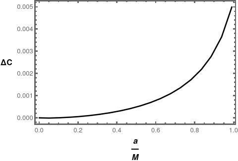
From the observation of the shadow of M87∗, the EHT collaboration has given a bound for an inclination angle Collaboration 2019a; Collaboration 2019b; Collaboration 2019c. However, the bound on from SgrA∗ is not available. From Fig. 6, we note that for Kerr black holes the maximum value for all inclination angles (). Considering the orientation of the observed relativistic jets from the M87∗, the inclination angle is estimated to be Walker et al. 2018. In Fig. 6, the variation of is shown as the function of . Note that the maximum value of for the inclination angle . For the same inclination angle, we scanned the parameter space for the dyonic Kerr-Sen black holes. From Fig. 7 we note that the for . As increases with the inclination angle , we have also scanned the parameter space for the inclination angle in Fig. 7. The maximum possible deviation is . Therefore, we conclude that all black hole parameters are allowed and the present observational bound on the deviation from circularity cannot constrain the parameter space of the dyonic Kerr-Sen black holes.


The recent EHT papers on SgrA∗ observations have used the fractional deviation parameter to constrain the spacetime geometries different from the Schwarzschild or Kerr black holes. The definition of is as follows
| (70) |
where the average diameter of the shadow , . Using the observations of the shadow of SgrA∗ and two separate sets of prior values of mass and distance of SgrA∗ from the VLTI and Keck observations, the EHT collaboration provided the bound on Collaboration 2022a; Collaboration 2022b as
| (71) |
Therefore, we get the common range of , , which is in the observational limits of both VLTI and Keck data.


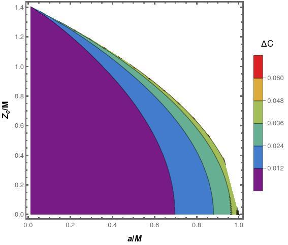
In Fig. 8, we scan the parameter space with the contours labeled by different values of for the Kerr black holes. It is noted that for all parameter values. Thus, the Kerr black hole parameters are unconstrained from the observational bound on from SgrA∗. Further, we note that the variation in is less sensitive to the variation of . Moreover, in the observation of SgrA∗, inclination angle greater than is disfavored.
Therefore, we choose in Fig. 9(a), where we scan the parameter space with contours of different values for the dyonic Kerr-Sen black holes. In the blue shaded region of the plot which means that the corresponding parameter values () are not allowed according to the observations of the SgrA∗. Further, we note that for a value greater than the critical limit , no value can satisfy the observational constraint. This critical value of is independent of the inclination angle as the critical limit corresponds to the , i.e. the static black hole. In Fig. 9(b), we show the variation of as a function of for static black holes, using the analytical expression for the shadow radius given in Eq. (62). There, we explicitly show the critical limit of . We conclude that and for any of allowed values, the allowed range of must be within the allowed region of space shown in Fig. 9(a). In other words, a value 0.873 is not allowed for any rotation parameter .
VI Comparison with other observations
Magnetic monopoles are a natural outcome of grand-unified theories (GUTs) Hooft 1974 and were among the original motivations for cosmic inflation Guth 1981; Preskill 1979. They have been searched for in various experiments Ambrosio et al. 2002; Orito et al. 1991; Balestra et al. 2008. Primordial black holes with magnetic charges, which have reached the extremality condition in the course of cosmic evolution and do not Hawking radiate anymore, can be a possible dark matter candidate Diamond and Kaplan 2022. They are termed as the extremal Magnetic Black Holes (EMBHs). Various astrophysical limits on such EMBHs were discussed in Diamond and Kaplan 2022. The authors in Diamond and Kaplan 2022 put constraints on such black holes with mass range having the upper limit . Therefore, these black holes cannot be used for modeling supermassive black holes such as M87∗ or SgrA∗. Hence, bounds obtained from observations of shadow images, as discussed in this article are not directly applicable to such EMBHs. However, we can develop some qualitative idea on what type of physical processes can indeed give bounds on any magnetic charge present in supermassive black holes such as the one at the center of our galaxy. In the following, we discuss two such possibilities.
From the observed temperature of clouds of Warm Ionized Medium (WIM) in the Milky Way Lehner et al. 2004, we can put some upper bound on the magnetic charge of SgrA*. Following the calculations of Diamond and Kaplan 2022, we get a rough estimate of a upper bound on any magnetic charge that may be present in SgrA∗. While the magnetized black hole passes through the surrounding plasma (WIM), the black hole deposits energy into the plasma. The rate of energy deposition is given by Diamond and Kaplan 2022
| (72) |
where is the magnetic charge (in the mass unit) of the black hole. Note that, in Diamond and Kaplan 2022 natural units are used. In these units, the magnetic charge is unit less and given by where the Planck mass . This process heats up the surrounding gas clouds. On the other hand, the observed cooling rate per unit volume for the WIM gas clouds in the Milky Way is
| (73) |
where is the typical number density of hydrogen atoms in the gas cloud. The low density WIM fills more than 20% of the volume within a 2 Kpc thick layer around the galactic midplane. These results have been derived from a relatively small number of sight lines that sample a region of radius 3-4 Kpc about the Sun Reynolds 1992. Therefore, around SgrA*, consider a region of disk of radius 8 Kpc (i.e. the distance from the Sun to the SgrA*) and thickness 2 Kpc. We assume that WIM clouds fill 20% of this region of space. So, the effective volume of WIM, . Therefore, the net cooling rate of WIM surrounding SgrA* up to the distance to the Sun is roughly . (Here, note that the cooling rate per unit volume may be different as we go far away beyond 3-4 Kpc from the Sun and near SgrA*. But for a rough estimate we can assume the cooling rate to be the same throughout the region of space we considered.) Now the heating rate given by Eq. (72) must be less than the net cooling rate, i.e.
| (74) |
Thus the bound on the magnetic charge . SgrA* has mass . Thus, .
Another astrophysical constraint comes from the Parker bound Parker 1970 which is based upon the survival of today’s galactic magnetic field, as the field energy is drained out by the magnetic monopoles while moving through the field. This puts an upper limit on the flux of magnetic monopoles. Monopoles moving through a magnetic field extract energy from the field at the rate causing dissipation of the field energy in the characteristic time
| (75) |
where is the magnetic current density and Gauss is the galactic magnetic field. years if the field can be regenerated in a time as short as years. The “Extended Parker bound” obtained by requiring survival and growth of a small galactic seed field after the collapse of the protogalaxy is Lewis et al. 2000
| (76) |
where is the flux of magnetic monopoles around the solar system and GeV. The magnetic current density , where is the magnetic charge density and is velocity of the charges. The flux of magnetic monopoles is . The relative velocity of the SgrA* with respect to the Solar System is km/sec and for the magnetic monopole charge of SgrA*. Thus the effective flux of magnetic charge of SgrA* around the solar system is
| (77) |
where (distance to the SgrA* from the Solar System). Therefore, and .
Clearly, the above astrophysical constraints seem to be far more stringent, by several orders of magnitude than the constraint obtained from shadow observations (i.e. the result ).
VII Discussion and conclusions
In this paper we have revisited black holes with dyonic charges in Einstein-Maxwell–dilaton-axion (EMDA) theory in the context of the observations on shadows of the supermassive black holes M87∗ and SgrA∗.
First we outlined the derivation of the static black hole solution by direct integration of the field equations of EMDA theory. Further, the rotating version (the dyonic Kerr-Sen black hole) was obtained from the static solution by applying the Newman-Janis algorithm. Thereafter, we analyzed the structure of the static black holes in detail. The differences with the standard Reissner-Nordström (RN) black holes are parametrized by the quantity . These static black holes have a single horizon (the event horizon) unlike non-extremal RN black holes. For either or the axion field vanishes. However the dilaton field vanishes only when both and , which is the case for the Schwarzschild black hole. Thus there is no solution with only axion and Maxwell’s electromagnetic field but without dilaton field. The reason lies in the structure of the EMDA action where the axion field is linearly coupled with . The static dyonic black holes satisfy all energy conditions outside the event horizon. There is also no stable photon orbit outside the event horizon of these static dyonic black holes.
For the rotating case () the axion field is nonzero even if the axion charge is zero () which is the case for the Kerr-Sen black hole (, , and ). In the static limit of the Kerr-Sen black holes (i.e. setting ), the axion field vanishes. This is an interesting difference between the Kerr-Sen black holes and the dyonic Kerr-Sen black holes, in general.
We study the shadow profiles for both rotating and static black holes. We have obtained the exact expression for the shadow radius for static black holes. The parameter and the shadow radius obeys . The effect of magnetic charge/ monopole on the shadow profile of rotating black holes has been investigated graphically by comparing the dyonic Kerr-Sen black holes with the Kerr-Newman and the Kerr-Sen black holes (Fig. 4). The deviation increases with the increase in magnetic charge. However, the deviation is not so prominent for higher rotation parameter (Fig. 5).
Finally, we test whether the known supermassive black holes at galactic centres could be modeled as such dyonic Kerr-Sen black holes. In other words, we look for metric parameter values for which the shadow features match with those in the observed shadow images of M87∗ and SgrA∗. We have used two observational quantities related to black hole shadows – the deviation from circularity of the observed shadow boundary () and the fractional deviation parameter () representing the deviation of the observed average shadow diameter from that for a Schwarzschild black hole. The observational bound on for M87∗ is satisfied for all parameter values for the dyonic black holes. Thus, it cannot be constrained. For SgrA∗, the EHT collaboration provided a bound on which gives a constraint on the black hole parameter . Thus we get an upper bound on the magnetic monopole charge (if any) for SgrA∗ as where for SgrA∗. In natural units, a magnetic charge where is the Planck mass. In these units, the obtained bound on the magnetic charge of SgrA∗ is .
In the literature any other observational constraint on the possibility of magnetic monopole charge of SgrA* does not exist. There are some astrophysical constraints on the Extremal Magnetic Black Holes (EMBHs), which are basically primordial black holes and dark matter candidates. But these constraints are not useful for SgrA* and M87* as the mass of the supermassive black holes are extremely high as compared to those EMBH mass ranges. However, in Section VI, we have estimated roughly the astrophysical constraints on the magnetic monopole charge of SgrA*, following arguments similar to those discussed in Diamond and Kaplan 2022. From the observed cooling rate of the WIM clouds in the Milky Way, we can get a rough estimate and from the Parker bound on the flux of the magnetic charges, we get an estimate . Both these estimates are more stringent by several orders of magnitude than those we obtained from the observed shadow of SgrA*. However, for M87* situated at a distance of 16.8 Mpc, similar astrophysical observations do not exist and hence similar constraints (as found for SgrA*) cannot be estimated.
Thus, at present, it is difficult to reach any definite conclusion about the viable presence/absence of magnetic monopole charges in the supermassive black holes such as M87* and SgrA*. Future observations of shadow images at greater experimental sensitivities and more concrete analysis of other astrophysical constraints may provide bounds which are closer in value to each other and hence more conclusive in nature. However, the theoretical analysis we have carried out is indeed new and may be of use once more imaging observations on shadows of black holes are carried out and presented in future.
Acknowledgements
The research of SJ is partially supported by the SERB, DST, Govt. of India, through a TARE fellowship grant no. TAR/2021/000354, hosted by the department of Physics, Indian Institute of Technology Kharagpur.
References
- Chen and Zhang (2013) B. Chen and J.-j. Zhang, Phys. Rev. D 87, 081505 (2013).
- Gibbons and Maeda (1988) G. W. Gibbons and K.-i. Maeda, Nucl. Phys. B 298, 741 (1988).
- Garfinkle et al. (1991) D. Garfinkle, G. T. Horowitz, and A. Strominger, Phys. Rev. D 43, 3140 (1991), [Erratum: Phys.Rev.D 45, 3888 (1992)].
- Sen (1992) A. Sen, Phys. Rev. Lett. 69, 1006 (1992), arXiv:hep-th/9204046 .
- Campbell et al. (1991) B. A. Campbell, N. Kaloper, and K. A. Olive, Phys. Lett. B 263, 364 (1991).
- Shapere et al. (1991) A. D. Shapere, S. Trivedi, and F. Wilczek, Mod. Phys. Lett. A 6, 2677 (1991).
- Kallosh and Ortín (1993) R. Kallosh and T. Ortín, Phys. Rev. D 48, 742 (1993).
- Collaboration (2019a) E. H. T. Collaboration, The Astrophysical Journal Letters 875, L1 (2019a).
- Collaboration (2019b) E. H. T. Collaboration, The Astrophysical Journal Letters 875, L5 (2019b).
- Collaboration (2019c) E. H. T. Collaboration, The Astrophysical Journal Letters 875, L6 (2019c).
- Collaboration (2022a) E. H. T. Collaboration, The Astrophysical Journal Letters 930, L12 (2022a).
- Collaboration (2022b) E. H. T. Collaboration, The Astrophysical Journal Letters 930, L17 (2022b).
- Hioki and Miyamoto (2008) K. Hioki and U. Miyamoto, Phys. Rev. D 78, 044007 (2008), arXiv:0805.3146 [gr-qc] .
- Xavier et al. (2020) S. V. M. C. B. Xavier, P. V. P. Cunha, L. C. B. Crispino, and C. A. R. Herdeiro, Int. J. Mod. Phys. D 29, 2041005 (2020), arXiv:2003.14349 [gr-qc] .
- Narang et al. (2020) A. Narang, S. Mohanty, and A. Kumar, (2020), arXiv:2002.12786 [gr-qc] .
- Cheng et al. (1994) G.-J. Cheng, R.-R. Hsu, and W.-F. Lin, J. Math. Phys. 35, 4839 (1994), arXiv:hep-th/9302065 .
- Shaikh (2019) R. Shaikh, Phys. Rev. D 100, 024028 (2019), arXiv:1904.08322 [gr-qc] .
- Banerjee et al. (2022) I. Banerjee, S. Sau, and S. SenGupta, (2022), arXiv:2207.06034 [gr-qc] .
- Banerjee et al. (2020a) I. Banerjee, S. Sau, and S. SenGupta, Phys. Rev. D 101, 104057 (2020a), arXiv:1911.05385 [gr-qc] .
- Hu et al. (2021) Z. Hu, Z. Zhong, P.-C. Li, M. Guo, and B. Chen, Phys. Rev. D 103, 044057 (2021).
- Lee et al. (2021) B.-H. Lee, W. Lee, and Y. S. Myung, Phys. Rev. D 103, 064026 (2021).
- Banerjee et al. (2020b) I. Banerjee, S. Chakraborty, and S. SenGupta, Phys. Rev. D 101, 041301 (2020b).
- Hou et al. (2021) Y. Hou, M. Guo, and B. Chen, Phys. Rev. D 104, 024001 (2021).
- Vagnozzi et al. (2022) S. Vagnozzi et al., (2022), arXiv:2205.07787 [gr-qc] .
- Cvetič et al. (2016) M. Cvetič, G. W. Gibbons, and C. N. Pope, Phys. Rev. D 94, 106005 (2016).
- Guo et al. (2022) G. Guo, Y. Lu, P. Wang, H. Wu, and H. Yang, arXiv 2212.12901 (2022).
- Newman and Janis (1965) E. T. Newman and A. I. Janis, J. Math. Phys. 6, 915 (1965).
- Newman et al. (1965) E. T. Newman, E. Couch, K. Chinnapared, A. Exton, A. Prakash, and R. Torrence, Journal of Mathematical Physics 6, 918 (1965).
- Drake and Szekeres (2000) S. P. Drake and P. Szekeres, Gen. Rel. Grav. 32, 445 (2000), arXiv:gr-qc/9807001 .
- Gal’tsov and Kechkin (1994) D. V. Gal’tsov and O. V. Kechkin, Phys. Rev. D 50, 7394 (1994).
- Wu et al. (2021) D. Wu, S.-Q. Wu, P. Wu, and H. Yu, Phys. Rev. D 103, 044014 (2021), arXiv:2010.13518 [gr-qc] .
- Perlick and Tsupko (2022) V. Perlick and O. Y. Tsupko, Phys. Rept. 947, 1 (2022), arXiv:2105.07101 [gr-qc] .
- Chang and Zhu (2021) Z. Chang and Q.-H. Zhu, Journal of Cosmology and Astroparticle Physics 2021, 003 (2021).
- Bardeen (1973) J. M. Bardeen, Proceedings, Ecole d’Eté de Physique Théorique: Les Astres Occlus : Les Houches, France, August, 1972, 215-240 , 215 (1973).
- Vazquez and Esteban (2004) S. E. Vazquez and E. P. Esteban, Nuovo Cim. B 119, 489 (2004), arXiv:gr-qc/0308023 .
- Grenzebach et al. (2014) A. Grenzebach, V. Perlick, and C. Lämmerzahl, Phys. Rev. D 89, 124004 (2014).
- Grenzebach et al. (2015) A. Grenzebach, V. Perlick, and C. Lämmerzahl, Int. J. Mod. Phys. D 24, 1542024 (2015), arXiv:1503.03036 [gr-qc] .
- Bambi et al. (2019) C. Bambi, K. Freese, S. Vagnozzi, and L. Visinelli, Phys. Rev. D 100, 044057 (2019), arXiv:1904.12983 [gr-qc] .
- Afrin et al. (2023) M. Afrin, S. Vagnozzi, and S. G. Ghosh, Astrophys. J. 944, 149 (2023), arXiv:2209.12584 [gr-qc] .
- Shaikh (2022) R. Shaikh, (2022), arXiv:2208.01995 [gr-qc] .
- Walker et al. (2018) R. C. Walker, P. E. Hardee, F. B. Davies, C. Ly, and W. Junor, The Astrophysical Journal 855, 128 (2018).
- Hooft (1974) G. Hooft, Nuclear Physics B 79, 276 (1974).
- Guth (1981) A. H. Guth, Phys. Rev. D 23, 347 (1981).
- Preskill (1979) J. P. Preskill, Phys. Rev. Lett. 43, 1365 (1979).
- Ambrosio et al. (2002) M. Ambrosio et al. (MACRO), Eur. Phys. J. C 25, 511 (2002), arXiv:hep-ex/0207020 .
- Orito et al. (1991) S. Orito et al., Phys. Rev. Lett. 66, 1951 (1991).
- Balestra et al. (2008) S. Balestra et al., Eur. Phys. J. C 55, 57 (2008), arXiv:0801.4913 [hep-ex] .
- Diamond and Kaplan (2022) M. D. Diamond and D. E. Kaplan, JHEP 03, 157 (2022), arXiv:2103.01850 [hep-ph] .
- Lehner et al. (2004) N. Lehner, B. P. Wakker, and B. D. Savage, Astrophys. J. 615, 767 (2004), arXiv:astro-ph/0407363 .
- Reynolds (1992) R. Reynolds, in AIP Conference Proceedings, Vol. 278 (American Institute of Physics, 1992) pp. 156–165.
- Parker (1970) E. N. Parker, Astrophys. J. 160, 383 (1970).
- Lewis et al. (2000) M. J. Lewis, K. Freese, and G. Tarle, Phys. Rev. D 62, 025002 (2000).