跳到论文正文
W Papers独立论文阅读器 arXiv:2303.14413 论文正文 计算阅读时间 · 0%
引用这篇论文根据当前论文元数据生成,正式投稿前建议核对。


License: arXiv.org perpetual non-exclusive license
arXiv:2303.14413v1 [gr-qc] 25 Mar 2023
\typearea

15

OCU-PHYS-480 AP-GR-145

The exact solutions to an Einstein-Dirac-Maxwell system with Sasakian quasi-Killing spinors on 4D spacetimes

Satsuki Matsuno11 1 smatsuno43@gmail.com
Fumihiro Ueno22 2 ueno-fumihiro-dx@alumni.osaka-u.ac.jp

Department of Physics, Graduate School of Science, Osaka Metropolitan University
3-3-138 Sugimoto, Sumiyoshi, Osaka 558-8585, Japan

Abstract

Exact solutions to an Einstein-Maxwell(E-D-M) system with an electric current are simple models of global cosmic magnetic phenomena in the universe. In this paper, we consider an E-D-M system with two chiral spinors ψ±\psi^{\pm} coupled with a gauge field AA and an electromagnetic field F=d​AF=dA. We construct a family of exact solutions to the E-D-M system on four-dimensional static Sasakian spacetimes. The electromagnetic field in the solutions is a contact magnetic field, and the chiral spinors are induced from Sasakian quasi-Killing spinors. We find closed universe models whose weak energy condition holds and open universe models whose weak energy condition is violated. In this study, we introduce the Sasakian frame, which is used to prospectively discuss the properties of Sasakian quasi-Killing spinors. A simple description of Sasakian quasi-Killing spinors of a certain type is obtained.

1 Introduction

In the real universe, there is a somewhat strong global magnetic field[1]. It is known that there is a strong magnetic field, then there may be an electric current. Such a system is composed of Einstein gravity, an electromagnetic field, and matter generating the current. Most of the systems are very complicated, and it is often difficult to find exact solutions without simplification.

So, it is interesting to constructing exact solutions to an Einstein-Maxwell system with an electric current. Many researchers have constructed exact solutions to Einstein-Maxwell systems with charged perfect fluids[2].

Ishihara and Matsuno (one of the present authors) constructed a family of exact solutions to an Einstein-Maxwell system with a charged dust fluid on a static Sasakian spacetime[3, 4]. The solutions are derived from matter consisting of a contact magnetic field and charged dust fluids flowing along Reeb orbits. However, as fluid is a composite object, it is expected that similar situations can be created by more fundamental matter, for example spinors or scalar fields.

In [6], on the four-dimensional static Einstein spacetime, a family of exact solutions to Dirac-Maxwell system is constructed. The spinor of the solutions generates an electric current which flows along fibers of the Hopf fibration of S3S^{3}. Inspired by this work, we generalize S3S^{3} to three-dimensional Sasakian manifolds and construct exact solutions to an Einstein-Dirac-Maxwell (E-D-M) system by considering spinors that generate an electric current along Reeb orbits.

In this paper, we consider an E-D-M system consisting of two chiral spinors ψ±\psi^{\pm} coupled with a gauge field AA and the electromagnetic field F=d​AF=dA. The action functional of the theory is given by

S=∫M(ℛ−14​‖F‖2+ℜ​𝔢⁡(ψ+¯​(D̸+−m+)​ψ+)+ℜ​𝔢⁡(ψ−¯​(D̸−−m−)​ψ−)−2​Λ)​volg.S=\int_{M}\left(\mathcal{R}-\frac{1}{4}||F||^{2}+\mathop{\mathfrak{Re}}\nolimits\left(\overline{\psi^{+}}(\not{D}^{+}-m^{+})\psi^{+}\right)+\mathop{\mathfrak{Re}}\nolimits\left(\overline{\psi^{-}}(\not{D}^{-}-m^{-})\psi^{-}\right)-2\Lambda\right)\operatorname{vol}_{g}.

Our strategy is to use a contact magnetic field and Sasakian quasi-Killing spinors for constructing exact solutions to the system. A contact magnetic field is a magnetic field whose gauge field is proportional to a contact form on contact manifolds, which was introduced in [7]. The motion of charged particles in contact magnetic fields and other geometrical properties have been studied in [7, 8, 9] (and references therein). However, few studies have investigated the relationship between a contact magnetic field and Einstein gravity. A Sasakian quasi-Killing spinor is a generalization of a Killing spinor in Sasakian geometry, which was introduced by Friedrich and Kim[10]. Killing spinors play an important role in supergravity and have been actively studied[11, 12, 13, 14] (and references therein). On the other hand, Sasakian quasi-Killing spinors seem to have few applications in mathematical physics. It is expected that using Sasakian quasi-Killing spinors rather than Killing spinors prescribes a rich solution space to Einstein gravity since the number of Sasakian quasi-Killing spinors is larger than that of Killing spinors on Sasakian manifolds.

We construct a family of exact solutions to the E-D-M system on static Sasakian spacetimes, which are direct product manifolds of time and a Sasakian 3-manifold. The matter fields in the solutions are a contact magnetic field and chiral spinors made from Sasakian quasi-Killing spinors. These solutions describe a situation where an electric current flows uniformly along one direction in space, generating a global cosmic magnetic field. There are closed universe models homeomorphic to ℝ×S3\mathbb{R}\times S^{3} whose weak energy condition holds and open universe models homeomorphic to ℝ×ℝ3\mathbb{R}\times\mathbb{R}^{3} whose weak energy condition is violated.

The organization of this paper is as follows. At the \hyperref[subsc:relusts]end of this section, we summarize the main results of this study. In Section 2 we describe our system in detail. We also review some facts about Sasakian geometry and Sasakian quasi-Killing spinors, and explain how to construct a spinor on a four-dimensional static Sasakian spacetime from spinors on a three-dimensional Sasakian manifold. Section 3 is devoted to solving our system. First, we introduce the Sasakian frame, which is used to prospectively discuss the properties of Sasakian quasi-Killing spinors and show some propositions. Next, after fully determining the solutions of the Einstein-Dirac system in our settings, we construct a family of exact solutions to our E-D-M system. Some of the calculations are described in Appendix B. Finally, in Section 4, the results of this paper are briefly summarized and the energy condition of spinors and possible future research are discussed.

Summary of the results

We summarize our results in Section 3.2. Let (N,ϕ,ξ,η,h)(N,\phi,\xi,\eta,h) be a three-dimensional Sasakian space form of ϕ\phi-sectional curvature HH, and let (M,g)(M,g) be a four-dimensional static spacetime defined by

M=ℝ×N,g=−d​t2+r2​h,r∈ℝ>0.M=\mathbb{R}\times N,\ g=-dt^{2}+r^{2}h,\ r\in\mathbb{R}_{>0}.

We consider the following matter fields on (M,g)(M,g). The electromagnetic field is F=d​AF=dA whose gauge field is given by A=B​η,B∈ℝA=B\eta,\ B\in\mathbb{R}. The massive spinor fields are ψ±=e−1​E​t​ϕR±⊕ϕL±\psi^{\pm}=e^{\sqrt{-1}Et}\phi_{R}^{\pm}\oplus\phi_{L}^{\pm} with charges ±q\pm q and masses m±>0m^{\pm}>0 respectively, where ϕP±,P=R,L\phi_{P}^{\pm},\ P=R,L are Sasakian quasi-Killing spinors of type (a,b)(a,b). Suppose (M,g),F(M,g),F and ψ±\psi^{\pm} satisfy the E-D-M system, that is,

Ric−12​ℛ​g+Λ​g=T≔Tem+Tspin,\displaystyle\operatorname{Ric}-\frac{1}{2}\mathcal{R}g+\Lambda g=T\coloneqq T^{\rm em}+T^{\rm spin}, (1.1)
(D̸±−m±)​ψ±=0,\displaystyle(\not{D}^{\pm}-m^{\pm})\psi^{\pm}=0, (1.2)
∗d∗F=(Jq(ψ+)+J−q(ψ−))♭,\displaystyle*d*F={}^{\flat}\left(J_{q}(\psi^{+})+J_{-q}(\psi^{-})\right), (1.3)

where Λ∈ℝ\Lambda\in\mathbb{R} is cosmological constant, D̸±\not{D}^{\pm} are Dirac operators of spin-c connection with respect to charge ±q\pm q, and J±q​(ψ±)J_{\pm q}(\psi^{\pm}) are the Dirac current of ψ±\psi^{\pm}. Then the solutions of the system for H≠−5H\neq-5 are given by

(a,b)\displaystyle(a,b) =(12,H−14),\displaystyle=\left(\frac{1}{2},\frac{H-1}{4}\right), (1.4)
‖ϕR+‖N2=‖ϕR−‖N2\displaystyle||\phi^{+}_{R}||_{N}^{2}=||\phi^{-}_{R}||_{N}^{2} =−B⁡(4​B​q+4​E​r+H+5)q​r3​(4​B​q+H+5),\displaystyle=-\frac{B\left(4Bq+4Er+H+5\right)}{qr^{3}(4Bq+H+5)}, (1.5)
‖ϕL+‖N2=‖ϕL−‖N2\displaystyle||\phi^{+}_{L}||_{N}^{2}=||\phi^{-}_{L}||_{N}^{2} =B⁡(4​B​q−4​E​r+H+5)q​r3​(4​B​q+H+5),\displaystyle=\frac{B\left(4Bq-4Er+H+5\right)}{qr^{3}\left(4Bq+H+5\right)}, (1.6)
(m+)2\displaystyle(m^{+})^{2} =−(H+4​B​q+5−4​r​E)​(H+4​B​q+5+4​E​r)16​r2,\displaystyle=-\frac{\left(H+4Bq+5-4rE\right)(H+4Bq+5+4Er)}{16r^{2}}, (1.7)
(m−)2\displaystyle(m^{-})^{2} =−(H−4​B​q+5−4​r​E)​(H−4​B​q+5+4​E​r)16​r2,\displaystyle=-\frac{\left(H-4Bq+5-4rE\right)\left(H-4Bq+5+4Er\right)}{16r^{2}}, (1.8)
B2\displaystyle B^{2} =(H−1)​(L+1)​r22​(H+5),\displaystyle=\frac{\left(H-1\right)\left(L+1\right)r^{2}}{2(H+5)}, (1.9)
q2\displaystyle q^{2} =(H+5)​(H−1)​(L+1)8​r2​(H−3​L+2)2,\displaystyle=\frac{(H+5)\left(H-1\right)\left(L+1\right)}{8r^{2}\left(H-3L+2\right)^{2}}, (1.10)
E2\displaystyle E^{2} =−(H2−2​H​L+6​H−4​L+11)​(H2−2​H​L+8​H−16​L+9)16​r2​(H−3​L+2)2,\displaystyle=-\frac{\left(H^{2}-2HL+6H-4L+11\right)\left(H^{2}-2HL+8H-16L+9\right)}{16r^{2}\left(H-3L+2\right)^{2}}, (1.11)

where L=Λ​r2L=\Lambda r^{2}, and the relation of the Sasakian space form NN and the range of H,LH,L and EE are given in the following table:

Table 1.1: The ranges of H,LH,L and EE
Range of HH Range of LL Sign of EE NN
(i) −8<H<−5-8<H<-5 h⁡(H)<L<∞h(H)<L<\infty Negative SL⁡(2,ℝ)~\widetilde{{\rm SL}(2,\mathbb{R})}
(ii) −5<H<−4-5<H<-4 k⁡(H)<L<−1k(H)<L<-1 Negative SL⁡(2,ℝ)~\widetilde{{\rm SL}(2,\mathbb{R})}
(iii) 1<H1<H h⁡(H)<L<k⁡(H)h(H)<L<k(H) Positive S3S^{3}

where k⁡(H)=H+22,h⁡(H)=H2+8​H+92​(H+8)k(H)=\frac{H+2}{2},\ h(H)=\frac{H^{2}+8H+9}{2(H+8)}.

2 The Einstein-Dirac-Maxwell system

First, we describe our E-D-M system. Let (M,g)(M,g) be a four-dimensional spacetime. We consider two spinors ψ±\psi^{\pm} coupled with a U⁡(1)U(1) gauge field AA and an electromagnetic field F=d​AF=dA. In this paper, we solve Euler-Lagrange equations of the following Lagrangian density of the E-D-M system

ℒ=ℛ−14​‖F‖2+(ψ+,(D̸+−m+)​ψ+)M+(ψ−,(D̸−−m−)​ψ−)M−2​Λ,\mathcal{L}=\mathcal{R}-\frac{1}{4}||F||^{2}+\left(\psi^{+},(\not{D}^{+}-m^{+})\psi^{+}\right)_{M}+\left(\psi^{-},(\not{D}^{-}-m^{-})\psi^{-}\right)_{M}-2\Lambda, (2.1)

where Λ\Lambda is a cosmological constant, ℛ\mathcal{R} is the scalar curvature, m±>0m^{\pm}>0 are masses of ψ±\psi^{\pm}, D̸±\not{D}^{\pm} are Dirac operators with respect to a spin-c connections ∇±q\nabla^{\pm}q for charges ±q\pm q, and (ψ1,ψ2)M=ℜ​𝔢⁡(ψ1¯​ψ2)\left(\psi_{1},\psi_{2}\right)_{M}=\mathop{\mathfrak{Re}}\nolimits(\overline{\psi_{1}}\psi_{2}). The Euler-Lagrange equations are Einstein, Dirac and Maxwell equations

Ric−12​ℛ​g+Λ​g=T≔Tem+Tspin,\displaystyle\operatorname{Ric}-\frac{1}{2}\mathcal{R}g+\Lambda g=T\coloneqq T^{\rm em}+T^{\rm spin}, (2.2)
(D̸±−m±)​ψ±=0,\displaystyle(\not{D}^{\pm}-m^{\pm})\psi^{\pm}=0, (2.3)
∗d∗F=(Jq(ψ+)+J−q(ψ−))♭,\displaystyle*d*F={}^{\flat}\left(J_{q}(\psi^{+})+J_{-q}(\psi^{-})\right), (2.4)

where the Dirac currents of ψ±\psi^{\pm} are defined by J±q​(ψ±)≔±q⁡(ψ±¯​γμ​ψ±)​XμJ_{\pm q}(\psi^{\pm})\coloneqq\pm q(\overline{\psi^{\pm}}\gamma^{\mu}\psi^{\pm})X_{\mu} using a global orthonormal frame {Xμ}μ=03\{X_{\mu}\}_{\mu=0}^{3} of (M,g).(M,g). The energy-momentum tensors of ψ±\psi^{\pm} are given by

Tψ±​(X,Y)=14​(ψ±,−1​X⋅∇Y±qψ±+−1​Y⋅∇X±qψ±)M,(X,Y∈Γ⁡(T​M)).T^{\psi^{\pm}}(X,Y)=\frac{1}{4}\left(\psi^{\pm},\sqrt{-1}X\cdot\nabla_{Y}^{\pm q}\psi^{\pm}+\sqrt{-1}Y\cdot\nabla_{X}^{\pm q}\psi^{\pm}\right)_{M},(X,Y\in\Gamma(TM)). (2.5)

Then the total energy-momentum tensor of spinors is written as Tspin=Tψ++Tψ−.T^{\rm spin}=T^{\psi^{+}}+T^{\psi^{-}}. The energy-momentum tensor of the electromagnetic field FF is given by

Tem​(X,Y)=g∗​(X​⌟​F,Y​⌟​F)−14​‖F‖2​g​(X,Y),(X,Y∈Γ⁡(T​M)).T^{\rm em}(X,Y)=g^{*}(X\lrcorner F,Y\lrcorner F)-\frac{1}{4}||F||^{2}g(X,Y),(X,Y\in\Gamma(TM)). (2.6)

Secondary, we review some basic facts about Sasakian geometry. The definition of Sasakian manifolds is as follows.

Definition 2.1.

A contact metric manifold is a quintuple (M,ϕ,ξ,η,g)(M,\phi,\xi,\eta,g) consisting of an odd dimensional manifold MM, a (1,1)(1,1)-type tensor field ϕ\phi, a vector field ξ\xi, a one-form η\eta and a Riemannian metric gg, which satisfies the following conditions.

ϕ2\displaystyle\phi^{2} =−id+η⊗ξ,\displaystyle=-\operatorname{id}+\eta\otimes\xi, (2.7)
η⁡(ξ)\displaystyle\eta(\xi) =1,\displaystyle=1, (2.8)
g⁡(ϕ​X,ϕ​Y)\displaystyle g(\phi X,\phi Y) =g⁡(X,Y)−η⁡(X)​η​(Y),\displaystyle=g(X,Y)-\eta(X)\eta(Y), (2.9)
g⁡(X,ϕ​Y)\displaystyle g(X,\phi Y) =d​η​(X,Y).\displaystyle=d\eta(X,Y). (2.10)

The quadruple (ϕ,ξ,η,g)(\phi,\xi,\eta,g) is called a contact metric structure of MM. The one-form η\eta and the vector field ξ\xi are called the contact form and the Reeb vector field of the contact metric structure. A contact manifold (M,ϕ,ξ,η,g)(M,\phi,\xi,\eta,g) is called a Sasakian manifold if the Riemann curvature tensor of (M,g)(M,g) satisfies R⁡(X,Y)​ξ=η⁡(Y)​X−η⁡(X)​YR(X,Y)\xi=\eta(Y)X-\eta(X)Y for arbitrary vector fields X,Y∈Γ⁡(T​M)X,Y\in\Gamma(TM).

It is known that a three-dimensional Riemannian manifold (M,g)(M,g) is a Sasakian manifold if and only if MM admits a unit Killing vector field ξ\xi and constant sectional curvature for any plane section including ξ\xi. For any vector field XX orthogonal to ξ\xi, the sectional curvature of the form H⁡(X)≔K⁡(X,ϕ⁡(X))H(X)\coloneqq K(X,\phi(X)) is called a ϕ−\phi-sectional curvature. A complete simply connected Sasakian manifold which has constant ϕ−\phi-sectional curvature is called a Sasakian space form.

Third, we introduce spacetimes which we investigated. Let (N,h)(N,h) be a three-dimensional simply connected Sasakian space form, and (M,g)(M,g) be a four-dimensional static spacetime defined by M=ℝ×NM=\mathbb{R}\times N and g=−d​t2+r2​h,g=-dt^{2}+r^{2}h, where tt is a coordinate of ℝ\mathbb{R} and rr is a positive constant. Because Sasakian space forms are all Lie groups, thus (N,h)(N,h) has a unique spin structure, therefore, (M,g)(M,g) also has a unique spin structure.

Finally, we introduce an ansatz of matter fields. We define a gauge field A=B​η,(B∈ℝ)A=B\eta,(B\in\mathbb{R}) using the contact form η\eta on N.N. Then the electromagnetic field FF is defined as F=d​A,F=dA, and since it is pure magnetic, it is called a contact magnetic field. Our two chiral spinors of spinor bundle SMS_{M} over (M,g)(M,g) are derived from Sasakian quasi-Killing spinors of spinor bundle SNS_{N} over (N,h)(N,h). A Sasakian quasi-Killing spinor is defined by Friedrich and Kim[10].

Definition 2.2.

A Sasakian quasi-Killing spinor of type (a,b)(a,b) is a non-trivial spinor field ϕ\phi which satisfies the following equation

∇XSNϕ=a​X⋅ϕ+b​η​(X)​ξ⋅ϕ,\nabla^{S_{N}}_{X}\phi=aX\cdot\phi+b\eta(X)\xi\cdot\phi, (2.11)

where, a,ba,b are real numbers and ∇SN\nabla^{S_{N}} is the spin connection induced from the Levi-Civita connection of (N,h)(N,h).

The spinor bundle SMS_{M} has a chiral decomposition SM=SMR⊕SMLS_{M}=S^{R}_{M}\oplus S^{L}_{M}. We have bundle isomorphisms SMP≃π∗​SN​(P=R,L)S_{M}^{P}\simeq\pi^{\ast}S_{N}\ (P=R,L) where π:M=ℝ×N→N\pi:M=\mathbb{R}\times N\to N is a projection map onto the second factor. Via these isomorphisms, we obtain two inclusion maps ιP:Γ⁡(SN)↪Γ⁡(SMR⊕SML)=Γ⁡(SM)\iota_{P}\colon\Gamma(S_{N})\hookrightarrow\Gamma(S^{R}_{M}\oplus S^{L}_{M})=\Gamma(S_{M}), that is, for ϕ∈Γ⁡(SN)\phi\in\Gamma(S_{N}), we define ιP​(ϕ)∈Γ⁡(SMP)\iota_{P}(\phi)\in\Gamma(S^{P}_{M}) as

ιR​(ϕ)=(ϕ0)∈Γ⁡(SMR),ιL​(ϕ)=(0ϕ)∈Γ⁡(SML).\displaystyle\iota_{R}(\phi)=\begin{pmatrix}\phi\\ 0\end{pmatrix}\in\Gamma(S^{R}_{M}),\ \iota_{L}(\phi)=\begin{pmatrix}0\\ \phi\end{pmatrix}\in\Gamma(S^{L}_{M}). (2.12)

For four Sasakian quasi-Killing spinors ϕP±​(P=R,L)\phi^{\pm}_{P}(P=R,L) of SNS_{N}, we can consider two chiral spinors ψ±\psi^{\pm} of SMS_{M}

ψ±≔e−1​E​t​(ιR​(ϕR±)+ιL​(ϕL±))=e−1​E​t​(ϕR±⊕ϕL±)=e−1​E​t​(ϕR±ϕL±),(E∈ℝ).\psi^{\pm}\coloneqq e^{\sqrt{-1}Et}\left(\iota_{R}(\phi^{\pm}_{R})+\iota_{L}(\phi^{\pm}_{L})\right)=e^{\sqrt{-1}Et}\left(\phi^{\pm}_{R}\oplus\phi^{\pm}_{L}\right)=e^{\sqrt{-1}Et}\begin{pmatrix}\phi^{\pm}_{R}\\ \phi^{\pm}_{L}\end{pmatrix},(E\in\mathbb{R}). (2.13)

To describe an interaction between charged spinors and gauge fields, we would like to introduce the spin-c connection. Let LL be a trivial complex line bundle and let A=B​η,B∈ℝA=B\eta,\ B\in\mathbb{R}. We define two connection forms ±−1​q​A\pm\sqrt{-1}qA on LL as gauge potentials. We identify the section of the spinor bundle SMS_{M} with a section of a trivial spin-c bundle Σ=SM⊗L\Sigma=S_{M}\otimes L. Let ∇±q=∇SM±−1​q​A\nabla^{\pm q}=\nabla^{S_{M}}\pm\sqrt{-1}qA be two connections on Σ\Sigma for charges ±q⁡(q>0).\pm q(q>0). Since the spin connection on SMS_{M} splits as ∇SM=∇SMR⊕∇SML,\nabla^{S_{M}}=\nabla^{S^{R}_{M}}\oplus\nabla^{S^{L}_{M}}, we obtain a connection decomposition on Σ=ΣR⊗ΣL​(ΣP=SMP⊗L)\Sigma=\Sigma^{R}\otimes\Sigma^{L}(\Sigma^{P}=S_{M}^{P}\otimes L) as

∇±q=(∇SMR±−1​q​A)⊕(∇SML±−1​q​A).\nabla^{\pm q}=(\nabla^{S^{R}_{M}}\pm\sqrt{-1}qA)\oplus(\nabla^{S^{L}_{M}}\pm\sqrt{-1}qA). (2.14)

We use Pauli matrices σi​(i=1,2,3)\sigma^{i}(i=1,2,3) as a basis of Lie algebra −1​𝔰​𝔬​(3)\sqrt{-1}\mathfrak{so}(3), i.e.

σ1=(0110),σ2=(0−−1−10),σ3=(100−1).\sigma^{1}=\begin{pmatrix}0&1\\ 1&0\end{pmatrix},\sigma^{2}=\begin{pmatrix}0&-\sqrt{-1}\\ \sqrt{-1}&0\end{pmatrix},\sigma^{3}=\begin{pmatrix}1&0\\ 0&-1\end{pmatrix}. (2.15)

The gamma matrices in the chiral representation are written as

γμ=(0σμσ¯μ0)⁡(μ=0,1,2,3),\gamma^{\mu}=\begin{pmatrix}0&\sigma^{\mu}\\ {\overline{\sigma}}^{\mu}&0\end{pmatrix}(\mu=0,1,2,3), (2.16)

where σ0=I2\sigma_{0}=I_{2} and (σ¯0,σ¯1,σ¯2,σ¯3)=(σ0,−σ1,−σ2,−σ3)({\overline{\sigma}}^{0},{\overline{\sigma}}^{1},{\overline{\sigma}}^{2},{\overline{\sigma}}^{3})=(\sigma^{0},-\sigma^{1},-\sigma^{2},-\sigma^{3}). Let D̸±=−1​∑μγμ​∇Xμ±q\not{D}^{\pm}=\sqrt{-1}\sum_{\mu}\gamma^{\mu}\nabla^{\pm q}_{X_{\mu}} be Dirac operators on Σ\Sigma using a global orthonormal frame {Xμ}μ=03\{X_{\mu}\}_{\mu=0}^{3} of (M,g).(M,g). The decomposition of Dirac operators

D̸±=(0D̸L±D̸R±0)\not{D}^{\pm}=\begin{pmatrix}0&\not{D}^{\pm}_{L}\\ \not{D}^{\pm}_{R}&0\end{pmatrix}\\ (2.17)

holds, where D̸R±=−1​∑μσ¯μ​(∇XμSMR±−1​q​A​(Xμ))\not{D}^{\pm}_{R}=\sqrt{-1}\sum_{\mu}{\overline{\sigma}}^{\mu}(\nabla^{S^{R}_{M}}_{X_{\mu}}\pm\sqrt{-1}qA(X_{\mu})) and D̸L±=−1​∑μσμ​(∇XμSML±−1​q​A​(Xμ))\not{D}^{\pm}_{L}=\sqrt{-1}\sum_{\mu}\sigma^{\mu}(\nabla^{S^{L}_{M}}_{X_{\mu}}\pm\sqrt{-1}qA(X_{\mu})).

Let ⟨ϕ1,ϕ2⟩N\left\langle\phi_{1},\phi_{2}\right\rangle_{N} denote a Hermitian metric on SNS_{N} for ϕi∈Γ⁡(SN),(i=1,2)\phi_{i}\in\Gamma(S_{N}),(i=1,2) and ⟨ψ1,ψ2⟩M=ψ1¯​ψ2\left\langle\psi_{1},\psi_{2}\right\rangle_{M}=\overline{\psi_{1}}\psi_{2} denote an invariant bilinear form on SMS_{M} for ψi∈Γ⁡(SM)​(i=1,2),\psi_{i}\in\Gamma(S_{M})(i=1,2), where ψ1¯≔ψ1†​γ0\overline{\psi_{1}}\coloneqq\psi_{1}^{\dagger}\gamma^{0} is the Dirac conjugate of ψ1∈Γ⁡(SM).\psi_{1}\in\Gamma(S_{M}). We also use brackets (∙,∙)N=ℜ​𝔢⁡⟨∙,∙⟩N\left(\bullet,\bullet\right)_{N}=\mathop{\mathfrak{Re}}\nolimits{\left\langle\bullet,\bullet\right\rangle_{N}} and (∙,∙)M=ℜ​𝔢⁡⟨∙,∙⟩M\left(\bullet,\bullet\right)_{M}=\mathop{\mathfrak{Re}}\nolimits{\left\langle\bullet,\bullet\right\rangle_{M}} and use the same symbols for Σ\Sigma.

3 Solutions to the Einstein-Dirac-Maxwell system

In this section, we solve our E-D-M system. We describe all solutions to our system except in the case H=−5H=-5.

3.1 Preparation for solving the E-D-M system

At first, we derive some basic formulae and propositions. three-dimensional Sasakian space forms are homogeneous and there are three kinds. They are decided by ϕ\phi-sectional curvature HH. A Sasakian space form is in Bianchi type IX if H>−3H>-3, type II if H=−3H=-3, or type VIII if H<−3H<-3. They are diffeomorphic to S3,Nil3,SL⁡(2,ℝ)~{\rm S}^{3},{\rm Nil}_{3},\widetilde{{\rm SL}(2,\mathbb{R})} respectively.

There is a useful global orthonormal frame on a Sasakian space form. On a three-dimensional Sasakian space form (N,ϕ,ξ,η,h)(N,\phi,\xi,\eta,h), there exists a global orthonormal frame {e1=ξ,e2,e3}\{e_{1}=\xi,e_{2},e_{3}\} which satisfies

[e1,e2]=−H+32​e3,[e1,e3]=H+32​e2,[e2,e3]=−2​e1,\displaystyle[e_{1},e_{2}]=-\frac{H+3}{2}e_{3},\ [e_{1},e_{3}]=\frac{H+3}{2}e_{2},\ [e_{2},e_{3}]=-2e_{1}, (3.1)

where HH is a ϕ\phi-sectional curvature (see Appendix A). We call this frame a Sasakian frame. The Ricci tensor of NN is given by

RicN=diag⁡(2,H+1,H+1),\displaystyle{\rm Ric}_{N}={\rm diag}(2,H+1,H+1), (3.2)

with respect to a Sasakian frame {e1,e2,e3}\{e_{1},e_{2},e_{3}\}.

We can define a global orthonormal frame {X0,X1,X2,X3}\{X_{0},X_{1},X_{2},X_{3}\} on (M,g)(M,g), where M=ℝ×NM=\mathbb{R}\times N and g=−d​t2+r2​hg=-dt^{2}+r^{2}h. That is, let {e1,e2,e3}\{e_{1},e_{2},e_{3}\} be a Sasakian frame on (N,h)(N,h) and put X0=∂t,Xi=1rei,(i=1,2,3)X_{0}=\partial_{t},\ X_{i}=\frac{1}{r}e_{i},\ (i=1,2,3). We also call this frame a Sasakian frame. Moreover the Ricci tensor of (M,g)(M,g) is given by

RicM=diag⁡(0,2r,H+1r,H+1r),\displaystyle{\rm Ric}_{M}={\rm diag}\left(0,\frac{2}{r},\frac{H+1}{r},\frac{H+1}{r}\right), (3.3)

with respect to a Sasakian frame {X0,X1,X2,X3}\{X_{0},X_{1},X_{2},X_{3}\}.

Let ∇N,∇M\nabla^{N},\nabla^{M} denote the Levi-Civita connections of N,MN,M respectively. The Levi-Civita connection ∇N\nabla^{N} is given by

∇eiNej=−∑k=13ciϵi​j​kek,(i,j∈{1,2,3}),\displaystyle\nabla^{N}_{e_{i}}e_{j}=-\sum_{k=1}^{3}c_{i}\epsilon_{ijk}e_{k},\ (i,j\in\{1,2,3\}), (3.4)

for a Sasakian frame {e1,e2,e3}\{e_{1},e_{2},e_{3}\}, where c1=H+12,c2=c3=1c_{1}=\frac{H+1}{2},\ c_{2}=c_{3}=1.

We denote the co-frame of {e1,e2,e3}\{e_{1},e_{2},e_{3}\} by {ω1=η,ω2,ω3}\{\omega^{1}=\eta,\omega^{2},\omega^{3}\}, where η\eta is the contact form of (N,h)(N,h). Hereafter we identify a pp-form α∈Ωp​(N)\alpha\in\Omega^{p}(N) and π∗​α∈Ωp​(M)\pi^{\ast}\alpha\in\Omega^{p}(M).

3.1.1 Formulae and Propositions for spinor fields

Here we give the connection form of the spinor bundle SMS_{M} and some basic propositions. We use a matrix representation of Clifford algebra ℂ​l3\mathbb{C}l_{3} written as

ei↦−1​σi≕si​(i=1,2,3),e_{i}\mapsto\sqrt{-1}\sigma_{i}\eqqcolon s_{i}\ (i=1,2,3), (3.5)

where {e1,e2,e3}\{e_{1},e_{2},e_{3}\} is a Sasakian frame on NN.

Lemma 3.1.

The spin connection form ωSN\omega^{S_{N}} of the spinor bundle SNS_{N} is given by

ωSN=12​∑k=13sk​ωk+H−14​s1​η,\displaystyle\omega^{S_{N}}=\frac{1}{2}\sum_{k=1}^{3}s_{k}\omega^{k}+\frac{H-1}{4}s_{1}\eta, (3.6)

with respect to a Sasakian frame {e1,e2,e3}\{e_{1},e_{2},e_{3}\}. Furthermore, the spin connection form ωSM\omega^{S_{M}} of the spinor bundle SMS_{M} is given by

ωSM=1r​ωSN⊕1r​ωSN.\displaystyle\omega^{S_{M}}=\frac{1}{r}\omega^{S_{N}}\oplus\frac{1}{r}\omega^{S_{N}}. (3.7)

Then, for ϕ∈Γ⁡(SN)\phi\in\Gamma(S_{N}), we have ∇SMιP​(ϕ)=ιP​(∇SNϕ)\nabla^{S_{M}}\iota_{P}(\phi)=\iota_{P}(\nabla^{S_{N}}\phi).

Proof.

The first claim follows from the simple calculation

ωSN\displaystyle\omega^{S_{N}} =14∑i,j,kh(∇eiej,ek)ωisjsk=−14∑i,j,kh(∇eiej,ek)ωiϵj​k​lsl\displaystyle=\frac{1}{4}\sum_{i,j,k}h(\nabla_{e_{i}}e_{j},e_{k})\omega^{i}s_{j}s_{k}=-\frac{1}{4}\sum_{i,j,k}h(\nabla_{e_{i}}e_{j},e_{k})\omega^{i}\epsilon_{jkl}s_{l}
=12​c3​ω3​s3+12​c2​ω2​s2+12​c1​ω1​s1\displaystyle=\frac{1}{2}c_{3}\omega^{3}s_{3}+\frac{1}{2}c_{2}\omega^{2}s_{2}+\frac{1}{2}c_{1}\omega^{1}s_{1}
=12​∑ksk​ωk+H−14​s1​η,\displaystyle=\frac{1}{2}\sum_{k}s_{k}\omega^{k}+\frac{H-1}{4}s_{1}\eta,

and the second claim is derived by

ωSM\displaystyle\omega^{S_{M}} =14​∑μ,ν,λg⁡(∇XμXν,Xλ)​ω~μ​γν​γλ=14​r​∑i,j,kh⁡(∇eiej,ek)​ω~i​γj​γk\displaystyle=\frac{1}{4}\sum_{\mu,\nu,\lambda}g(\nabla_{X_{\mu}}X_{\nu},X_{\lambda})\tilde{\omega}^{\mu}\gamma^{\nu}\gamma^{\lambda}=\frac{1}{4r}\sum_{i,j,k}h(\nabla_{e_{i}}e_{j},e_{k})\tilde{\omega}^{i}\gamma^{j}\gamma^{k} (3.8)
=14​r​∑i,j,kh⁡(∇eiej,ek)​ω~i​(sj​sk⊕sj​sk)=1r​ωSN⊕1r​ωSN,\displaystyle=\frac{1}{4r}\sum_{i,j,k}h(\nabla_{e_{i}}e_{j},e_{k})\tilde{\omega}^{i}(s_{j}s_{k}\oplus s_{j}s_{k})=\frac{1}{r}\omega^{S_{N}}\oplus\frac{1}{r}\omega^{S_{N}}, (3.9)

where {ω~μ}\{\tilde{\omega}^{\mu}\} is the co-frame of a Sasakian frame {Xμ}\{X_{\mu}\}. ∎

Using a Sasakian frame {e1,e2,e3}\{e_{1},e_{2},e_{3}\}, an invariant Hermitian metric is given by ⟨ϕ1,ϕ2⟩N=ϕ1†​ϕ2\langle\phi_{1},\phi_{2}\rangle_{N}=\phi_{1}^{\dagger}\phi_{2} and the Dirac current of ϕ∈Γ⁡(SN)\phi\in\Gamma(S_{N}) is given by JN(ϕ)≔−∑i−1⟨ϕ,siϕ⟩NeiJ_{N}(\phi)\coloneqq-\sum_{i}\sqrt{-1}\langle\phi,s_{i}\phi\rangle_{N}e_{i}. We denote ∑iJN​(ϕ)i\sum_{i}J_{N}(\phi)_{i} for an i-th component of JN​(ϕ)J_{N}(\phi).

Friedrich and Kim have classified Sasakian quasi-Killing spinors on three-dimensional Sasakian space forms as follows[10].

Proposition 3.2.

On three-dimensional Sasakian space forms with ϕ\phi-sectional curvature HH, there exists a Sasakian quasi-Killing spinor of type (12,H−14)\left(\frac{1}{2},\frac{H-1}{4}\right). Moreover, if H>−3H>-3 then there exists a Sasakian quasi-Killing spinor of type (1∓3+H2,−2∓3+H2)\left(\frac{1\mp\sqrt{3+H}}{2},-\frac{2\mp\sqrt{3+H}}{2}\right). In particular, if H=−3−52H=-\frac{3-\sqrt{5}}{2} then there exists a Sasakian quasi-Killing spinor of type (−3+54,5+54)\left(-\frac{3+\sqrt{5}}{4},\frac{5+\sqrt{5}}{4}\right), and if H=−3+52H=-\frac{3+\sqrt{5}}{2} then there exists a Sasakian quasi-Killing spinor of type (−3−54,5−54)\left(-\frac{3-\sqrt{5}}{4},\frac{5-\sqrt{5}}{4}\right).

The connection form (3.6) enables us to obtain a simple description of a Sasakian quasi-Killing spinor of type (12,H−14)\left(\frac{1}{2},\frac{H-1}{4}\right) as follows.

Proposition 3.3.

A spinor ϕ∈Γ⁡(SN)\phi\in\Gamma(S_{N}) is a Sasakian quasi-Killing spinor of type (12,H−14)\left(\frac{1}{2},\frac{H-1}{4}\right) if and only if ϕ=(αβ),α,β∈ℂ\phi=\begin{pmatrix}\alpha\\ \beta\end{pmatrix},\ \alpha,\beta\in\mathbb{C} with respect to a Sasakian frame {e1,e2,e3}\{e_{1},e_{2},e_{3}\}.

We decompose the spinor bundle SNS_{N} as well as Friedrich. The spinor bundle SNS_{N} splits into the orthogonal direct sum SN=Σ0⊕Σ1S_{N}=\Sigma_{0}\oplus\Sigma_{1} with ξ|Σ0=−−1​Id,ξ|Σ1=−1​Id\xi|_{\Sigma_{0}}=-\sqrt{-1}\ {\rm Id},\ \xi|_{\Sigma_{1}}=\sqrt{-1}\ {\rm Id}. Sections χ0∈Γ⁡(Σ0)\chi_{0}\in\Gamma(\Sigma_{0}) and χ1∈Γ⁡(Σ1)\chi_{1}\in\Gamma(\Sigma_{1}) are given by χ0=f0​(1−1)\chi_{0}=f_{0}\begin{pmatrix}1\\ -1\end{pmatrix} and χ1=f1​(11)\chi_{1}=f_{1}\begin{pmatrix}1\\ 1\end{pmatrix} for f0,f1∈C∞​(N)f_{0},f_{1}\in C^{\infty}(N) with respect to a Sasakian frame since we have ξ⋅=s1=(0−1−10)\xi\cdot=s_{1}=\begin{pmatrix}0&\sqrt{-1}\\ \sqrt{-1}&0\end{pmatrix} by (3.5). In particular, a Sasakian quasi-Killing spinor of type (12,H−14)\left(\frac{1}{2},\frac{H-1}{4}\right) is in Γ⁡(Σ0⊕Σ1)\Gamma(\Sigma_{0}\oplus\Sigma_{1}) from Proposition 3.3.

3.1.2 Formulae of the electromagnetic field

Here we explicitly write down the Maxwell equation (2.4) and the energy-momentum tensor of the electromagnetic field (2.6).

Since A=B​ηA=B\eta and F=d​A,F=dA, we have

∗d∗F\displaystyle\ast d\ast F =∗d∗(2Bω2∧ω3)=∗d(2​Brω0∧ω1)\displaystyle=\ast d\ast(2B\omega^{2}\wedge\omega^{3})=\ast d\left(\frac{2B}{r}\omega^{0}\wedge\omega^{1}\right)
=∗(−4​Brω0∧ω2∧ω3)=4​Br2ω1,\displaystyle=\ast\left(-\frac{4B}{r}\omega^{0}\wedge\omega^{2}\wedge\omega^{3}\right)=\frac{4B}{r^{2}}\omega^{1}, (3.10)

it follows that the Maxwell equation (2.4) is given by

4​Br3​X1=Jq​(ψ+)+J−q​(ψ−).\displaystyle\frac{4B}{r^{3}}X_{1}=J_{q}(\psi^{+})+J_{-q}(\psi^{-}). (3.11)

By simple calculation, we have the energy-momentum tensor of FF as follows

Tem=2​B2r4​diag​(1,−1,1,1),\displaystyle T^{\rm em}=\frac{2B^{2}}{r^{4}}{\rm diag}(1,-1,1,1), (3.12)

with respect to a Sasakian frame {X0,X1,X2,X3}\{X_{0},X_{1},X_{2},X_{3}\}.

3.1.3 Basic propositions of the Dirac-Maxwell system

In our settings, Maxwell equation (2.4) uniquely decides the type of Sasakian quasi-Killing spinors. First, we consider the derivative of the components of the Dirac current of a Sasakian quasi-Killing spinor as follows.

Lemma 3.4.

Let NN be a three-dimensional Sasakian space form, and let {e1,e2,e3}\{e_{1},e_{2},e_{3}\} be a Sasaian frame. For a Sasakian quasi-Killing spinor ϕ\phi of type (a,b)(a,b), the derivative of the scalar function JN​(ϕ)iJ_{N}(\phi)_{i} is given by

ej​(JN​(ϕ)i)=∑k(2​a​ϵj​i​k+2​b​η​(ej)​ϵi​1​k−cj​ϵj​i​k)​JN​(ϕ)k,\displaystyle e_{j}(J_{N}(\phi)_{i})=\sum_{k}(2a\epsilon_{jik}+2b\eta(e_{j})\epsilon_{i1k}-c_{j}\epsilon_{jik})J_{N}(\phi)_{k}, (3.13)

especially e3​(JN​(ϕ)2)=(−2​a+1)​JN​(ϕ)1e_{3}(J_{N}(\phi)_{2})=(-2a+1)J_{N}(\phi)_{1} holds.

Proof.
ej​(JN​(ϕ)i)\displaystyle e_{j}(J_{N}(\phi)_{i}) =−1​⟨∇jϕ,si​ϕ⟩N+−1​⟨ϕ,(∇jei)​ϕ⟩N+−1​⟨ϕ,si​∇jϕ⟩N\displaystyle=\sqrt{-1}\langle\nabla_{j}\phi,s_{i}\phi\rangle_{N}+\sqrt{-1}\langle\phi,(\nabla_{j}e_{i})\phi\rangle_{N}+\sqrt{-1}\langle\phi,s_{i}\nabla_{j}\phi\rangle_{N}
OPEN=a​−1​⟨sj​ϕ,si​ϕ⟩N+a​−1​⟨ϕ,si​sj​ϕ⟩N)+b​η​(ej)​−1​⟨s1​ϕ,si​ϕ⟩N\displaystyle=a\sqrt{-1}\langle s_{j}\phi,s_{i}\phi\rangle_{N}+a\sqrt{-1}\langle\phi,s_{i}s_{j}\phi\rangle_{N})+b\eta(e_{j})\sqrt{-1}\langle s_{1}\phi,s_{i}\phi\rangle_{N}
+b​−1​η​(ej)​⟨ϕ,si​s1​ϕ⟩N+−1​⟨ϕ,(∇ejei)​ϕ⟩N\displaystyle+b\sqrt{-1}\eta(e_{j})\langle\phi,s_{i}s_{1}\phi\rangle_{N}+\sqrt{-1}\langle\phi,(\nabla_{e_{j}}e_{i})\phi\rangle_{N}
=a​−1​⟨ϕ,−sj​si+si​sj​ϕ⟩N+b​−1​η​(ej)​⟨ϕ,−s1​si+si​s1​ϕ⟩N\displaystyle=a\sqrt{-1}\langle\phi,-s_{j}s_{i}+s_{i}s_{j}\phi\rangle_{N}+b\sqrt{-1}\eta(e_{j})\langle\phi,-s_{1}s_{i}+s_{i}s_{1}\phi\rangle_{N}
+−1​⟨ϕ,(∇ejei)​ϕ⟩N\displaystyle+\sqrt{-1}\langle\phi,(\nabla_{e_{j}}e_{i})\phi\rangle_{N}
=2​a​∑kϵj​i​k​JN​(ϕ)k+2​b​η​(ej)​∑kϵi​1​k​JN​(ϕ)k−cj​∑kϵj​i​k​JN​(ϕ)k\displaystyle=2a\sum_{k}\epsilon_{jik}J_{N}(\phi)_{k}+2b\eta(e_{j})\sum_{k}\epsilon_{i1k}J_{N}(\phi)_{k}-c_{j}\sum_{k}\epsilon_{jik}J_{N}(\phi)_{k}
(we usedsisj=−δi​j−∑kϵi​j​kskand∇eiej=−∑kciϵi​j​kek)\displaystyle(\text{we used}\ s_{i}s_{j}=-\delta_{ij}-\sum_{k}\epsilon_{ijk}s_{k}{\rm\ and\ }\nabla_{e_{i}}e_{j}=-\sum_{k}c_{i}\epsilon_{ijk}e_{k})
=∑k(2​a​ϵj​i​k+2​b​η​(ej)​ϵi​1​k−cj​ϵj​i​k)​JN​(ϕ)k\displaystyle=\sum_{k}(2a\epsilon_{jik}+2b\eta(e_{j})\epsilon_{i1k}-c_{j}\epsilon_{jik})J_{N}(\phi)_{k} (3.14)

∎

Then the following proposition holds.

Proposition 3.5.

Let ψ±∈Γ⁡(Σ)\psi^{\pm}\in\Gamma(\Sigma) be two chiral spinors with charge ±q\pm q defined by (2.13). If ψ±\psi^{\pm} and AA satisfy the Maxwell equation (2.4), then (a,b)=(12,H−14)(a,b)=\left(\frac{1}{2},\frac{H-1}{4}\right).

Proof.

Since (3.11), the current Jq​(ψ+)+J−q​(ψ−)J_{q}(\psi^{+})+J_{-q}(\psi^{-}) is proportional to ξ\xi, so we have

J1\displaystyle J_{1} ≔Jq​(ψ+)1+J−q​(ψ−)1=q⁡(−JN​(ϕR+)1+JN​(ϕL+)1+JN​(ϕR−)1−JN​(ϕL−)1)≠0,\displaystyle\coloneqq J_{q}(\psi^{+})_{1}+J_{-q}(\psi^{-})_{1}=q(-J_{N}(\phi^{+}_{R})_{1}+J_{N}(\phi^{+}_{L})_{1}+J_{N}(\phi^{-}_{R})_{1}-J_{N}(\phi^{-}_{L})_{1})\neq 0, (3.15)
J2\displaystyle J_{2} ≔Jq​(ψ+)2+J−q​(ψ−)2=q⁡(−JN​(ϕR+)2+JN​(ϕL+)2+JN​(ϕR−)2−JN​(ϕL−)2)=0,\displaystyle\coloneqq J_{q}(\psi^{+})_{2}+J_{-q}(\psi^{-})_{2}=q(-J_{N}(\phi^{+}_{R})_{2}+J_{N}(\phi^{+}_{L})_{2}+J_{N}(\phi^{-}_{R})_{2}-J_{N}(\phi^{-}_{L})_{2})=0, (3.16)

and furthermore e3​(J2)=0e_{3}(J_{2})=0 must holds. Since Lemma 3.4, we have

e3​(J2)\displaystyle e_{3}(J_{2}) =q⁡(−2​a+1)​(−JN​(ϕR+)1+JN​(ϕL+)1+JN​(ϕR−)1−JN​(ϕL−)1)\displaystyle=q(-2a+1)(-J_{N}(\phi^{+}_{R})_{1}+J_{N}(\phi^{+}_{L})_{1}+J_{N}(\phi^{-}_{R})_{1}-J_{N}(\phi^{-}_{L})_{1})
=q⁡(−2​a+1)​J1.\displaystyle=q(-2a+1)J_{1}. (3.17)

therefore we have a=12a=\frac{1}{2}. By Proposition 3.2, the classification result by Friedrich and Kim, b=H−14b=\frac{H-1}{4} holds. ∎

Remark 3.6.

From Equation 3.13 we have e1​(JN​(ϕ)2)=(2​a−2​b−c1)​JN​(ϕ)3,e1​(JN​(ϕ)3)=(−2​a+2​b+c1)​JN​(ϕ)2,e2​(JN​(ϕ)3)=(2​a−1)​JN​(ϕ)1,e3​(JN​(ϕ)2)=(−2​a+1)​JN​(ϕ)1,e2​(JN​(ϕ)2)=e3​(JN​(ϕ)3)=0e_{1}(J_{N}(\phi)_{2})=(2a-2b-c_{1})J_{N}(\phi)_{3},\ e_{1}(J_{N}(\phi)_{3})=(-2a+2b+c_{1})J_{N}(\phi)_{2},\ e_{2}(J_{N}(\phi)_{3})=(2a-1)J_{N}(\phi)_{1},\ e_{3}(J_{N}(\phi)_{2})=(-2a+1)J_{N}(\phi)_{1},\ e_{2}(J_{N}(\phi)_{2})=e_{3}(J_{N}(\phi)_{3})=0. Thus, in the case (a,b)=(12,H−14)(a,b)=\left(\frac{1}{2},\frac{H-1}{4}\right), if JN​(ϕ)2=JN​(ϕ)3=0J_{N}(\phi)_{2}=J_{N}(\phi)_{3}=0 at an arbitrary point then JN​(ϕ)2=JN​(ϕ)3=0J_{N}(\phi)_{2}=J_{N}(\phi)_{3}=0 on the whole of NN. Then JN​(ϕ)J_{N}(\phi) is a Killing vector field because Equation 3.13 implies (∇ejJN​(ϕ))i=∑k(2​a​ϵj​i​k+2​b​η​(ej)​ϵi​1​k)​JN​(ϕ)k(\nabla_{e_{j}}J_{N}(\phi))_{i}=\sum_{k}(2a\epsilon_{jik}+2b\eta(e_{j})\epsilon_{i1k})J_{N}(\phi)_{k}. Thus, on a three-dimensional Sasakian space form with H≠1H\neq 1, a Sasakian quasi-Killing spinor ϕ\phi of type (12,H−14)\left(\frac{1}{2},\frac{H-1}{4}\right) with JN​(ϕ)2=JN​(ϕ)3=0J_{N}(\phi)_{2}=J_{N}(\phi)_{3}=0 is an example of a non-Killing spinor whose Dirac current is a Killing vector field. If H=1H=1, it is a Killing spinor.

As we intend to show in Proposition 3.9, the Dirac equation leads to that ϕP±\phi_{P}^{\pm} are in Γ⁡(Σ0)\Gamma(\Sigma_{0}) or Γ⁡(Σ1)\Gamma(\Sigma_{1}). Given this fact, a more concrete representation of Maxwell’s equations is as follows.

Proposition 3.7.

Let ψ±∈Γ⁡(Σ)\psi^{\pm}\in\Gamma(\Sigma) be two chiral spinors with charge ±q\pm q defined by (2.13). If Sasakian quasi-Killing spinors ϕP±,P∈{R,L}\phi^{\pm}_{P},\ P\in\{R,L\} of type (12,H−14)\left(\frac{1}{2},\frac{H-1}{4}\right) are in Γ⁡(Σℓ±),ℓ±∈{0,1}\Gamma(\Sigma_{\ell_{\pm}}),\ \ell_{\pm}\in\{0,1\}, then the Maxwell equation (2.4) is given by

‖ϕR+‖N2+‖ϕL+‖N2−||ϕR−||N2−‖ϕL−‖N2=0,\displaystyle||\phi^{+}_{R}||_{N}^{2}+||\phi^{+}_{L}||_{N}^{2}-||\phi^{-}_{R}||_{N}^{2}-||\phi^{-}_{L}||_{N}^{2}=0, (3.18)
(−1)ℓ+​‖ϕR+‖N2−(−1)ℓ+​‖ϕL+‖N2−(−1)ℓ−||ϕR−||N2+(−1)ℓ−​‖ϕL−‖N2=4​Bq​r3\displaystyle(-1)^{\ell_{+}}||\phi^{+}_{R}||_{N}^{2}-(-1)^{\ell_{+}}||\phi^{+}_{L}||_{N}^{2}-(-1)^{\ell_{-}}||\phi^{-}_{R}||_{N}^{2}+(-1)^{\ell_{-}}||\phi^{-}_{L}||_{N}^{2}=\frac{4B}{qr^{3}} (3.19)
Proof.

By the assumptions, we have

ϕR±=αR±(1(−1)1+ℓ±),ϕL±=αL±(1(−1)1+ℓ±),αR±,αL±∈ℂ.\displaystyle\phi_{R}^{\pm}=\alpha_{R}^{\pm}\begin{pmatrix}1\\ (-1)^{1+\ell_{\pm}}\end{pmatrix},\ \phi_{L}^{\pm}=\alpha_{L}^{\pm}\begin{pmatrix}1\\ (-1)^{1+\ell_{\pm}}\end{pmatrix},\ \alpha_{R}^{\pm},\alpha_{L}^{\pm}\in\mathbb{C}. (3.20)

Then we obtain

Jq​(ψ+)+J−q​(ψ−)\displaystyle J_{q}(\psi^{+})+J_{-q}(\psi^{-}) =q⁡(⟨ψ+,γ0​ψ+⟩M−⟨ψ−,γ0​ψ−⟩M)​X0+q⁡(⟨ψ+,γ1​ψ+⟩M−⟨ψ−,γ1​ψ−⟩M)​X1\displaystyle=q\left(\langle\psi^{+},\gamma^{0}\psi^{+}\rangle_{M}-\langle\psi^{-},\gamma^{0}\psi^{-}\rangle_{M}\right)X_{0}+q\left(\langle\psi^{+},\gamma^{1}\psi^{+}\rangle_{M}-\langle\psi^{-},\gamma^{1}\psi^{-}\rangle_{M}\right)X_{1}
=2​q​(|αR+|2+|αL+|2−|αR−|2−|αL−|2)​X0\displaystyle=2q\left(|\alpha_{R}^{+}|^{2}+|\alpha_{L}^{+}|^{2}-|\alpha_{R}^{-}|^{2}-|\alpha_{L}^{-}|^{2}\right)X_{0}
+2​q​((−1)ℓ+​(|αR+|2−|αL+|2)−(−1)ℓ−​(|αR−|2−|αL−|2))​X1\displaystyle+2q\left((-1)^{\ell_{+}}(|\alpha_{R}^{+}|^{2}-|\alpha_{L}^{+}|^{2})-(-1)^{\ell_{-}}(|\alpha_{R}^{-}|^{2}-|\alpha_{L}^{-}|^{2})\right)X_{1}
=q⁡(||ϕR+||N2+‖ϕL+‖N2−‖ϕR−‖N2−|​|ϕL−||N2)​X0\displaystyle=q\left(||\phi^{+}_{R}||_{N}^{2}+||\phi^{+}_{L}||_{N}^{2}-||\phi^{-}_{R}||_{N}^{2}-||\phi^{-}_{L}||_{N}^{2}\right)X_{0}
+q⁡((−1)ℓ+​||ϕR+||N2−(−1)ℓ+​‖ϕL+‖N2−(−1)ℓ−​‖ϕR−‖N2+(−1)ℓ−|​|ϕL−||N2)​X1,\displaystyle+q\left((-1)^{\ell_{+}}||\phi^{+}_{R}||_{N}^{2}-(-1)^{\ell_{+}}||\phi^{+}_{L}||_{N}^{2}-(-1)^{\ell_{-}}||\phi^{-}_{R}||_{N}^{2}+(-1)^{\ell_{-}}||\phi^{-}_{L}||_{N}^{2}\right)X_{1},

which implies the claim. ∎

Next we write down the Dirac equation (2.3).

Proposition 3.8.

Let ψ±∈Γ⁡(Σ)\psi^{\pm}\in\Gamma(\Sigma) be two chiral spinors with charge ±q\pm q defined by (2.13). The Dirac equations (D̸±−m±)​ψ±=0(\not{D}^{\pm}-m^{\pm})\psi^{\pm}=0 are equivalent to the following linear equations

DR±​ϕR±\displaystyle D^{\pm}_{R}\phi^{\pm}_{R} =m±​ϕL±,\displaystyle=m^{\pm}\phi^{\pm}_{L}, (3.21)
DL±​ϕL±\displaystyle D^{\pm}_{L}\phi^{\pm}_{L} =m±​ϕR±,\displaystyle=m^{\pm}\phi^{\pm}_{R}, (3.22)

where DR±=(−E+3​a+br)​I2∓q​Br​σ1D^{\pm}_{R}=\left(-E+\frac{3a+b}{r}\right)I_{2}\mp\frac{qB}{r}\sigma_{1} and DL±=(−E−3​a+br)​I2∓q​Br​σ1.D^{\pm}_{L}=\left(-E-\frac{3a+b}{r}\right)I_{2}\mp\frac{qB}{r}\sigma_{1}.

Proof.

We can verify it by simple calculation,

D̸±​ψ±\displaystyle\not{D}^{\pm}\psi^{\pm} =(0−1​σμ​(∇XμSML±−1​q​A​(Xμ))−1​σ¯μ​(∇XμSMR±−1​q​A​(Xμ))0)​ψ±\displaystyle=\begin{pmatrix}0&\sqrt{-1}\sigma^{\mu}\left(\nabla^{S^{L}_{M}}_{X_{\mu}}\pm\sqrt{-1}qA(X_{\mu})\right)\\ \sqrt{-1}{\overline{\sigma}}^{\mu}\left(\nabla^{S^{R}_{M}}_{X_{\mu}}\pm\sqrt{-1}qA(X_{\mu})\right)&0\end{pmatrix}\psi^{\pm}
=(0−E−(3​a+b)/r∓q​Br​σ1−E+(3​a+b)/r±q​Br​σ10)​ψ±.\displaystyle=\begin{pmatrix}0&-E-(3a+b)/r\mp\frac{qB}{r}\sigma_{1}\\ -E+(3a+b)/r\pm\frac{qB}{r}\sigma_{1}&0\end{pmatrix}\psi^{\pm}. (3.23)

∎

3.2 Solutions to the E-D-M system

In this section, we begin by fully determining the solutions to our D-M system. It then becomes clear that there are two cases whether H=−5H=-5 or not and that the solutions to the D-M system are quite different for each case. Then, after calculating the energy-momentum tensor of the spinors, we solve to our E-D-M system for the case of H≠−5H\neq-5.

Proposition 3.9.

Let ψ±∈Γ⁡(Σ)\psi^{\pm}\in\Gamma(\Sigma) be two chiral spinors with charge ±q\pm q defined by (2.13). Suppose that ψ±\psi^{\pm} and AA satisfy the D-M system then the following hold.

  1. (I)

    In the case of H≠−5H\neq-5, we have ϕP±∈Γ⁡(Σℓ±),ℓ±∈{0,1}\phi^{\pm}_{P}\in\Gamma(\Sigma_{\ell_{\pm}}),\ \ell_{\pm}\in\{0,1\}. Especially,

    1. (i)

      if (ℓ+,ℓ−)=(1,0)(\ell_{+},\ell_{-})=(1,0), we have

      ‖ϕR+‖N2=‖ϕR−‖N2\displaystyle||\phi^{+}_{R}||_{N}^{2}=||\phi^{-}_{R}||_{N}^{2} =−B⁡(4​B​q+4​E​r+H+5)q​r3​(4​B​q+H+5),\displaystyle=-\frac{B\left(4Bq+4Er+H+5\right)}{qr^{3}(4Bq+H+5)}, (3.24)
      ‖ϕL+‖N2=‖ϕL−‖N2\displaystyle||\phi^{+}_{L}||_{N}^{2}=||\phi^{-}_{L}||_{N}^{2} =B⁡(4​B​q−4​E​r+H+5)q​r3​(4​B​q+H+5),\displaystyle=\frac{B\left(4Bq-4Er+H+5\right)}{qr^{3}\left(4Bq+H+5\right)}, (3.25)
    2. (ii)

      if (ℓ+,ℓ−)=(0,0)(\ell_{+},\ell_{-})=(0,0), we have

      ‖ϕR+‖N2\displaystyle||\phi^{+}_{R}||_{N}^{2} =4​B​q−4​E​r−H−54​q2​r3,‖ϕR−‖N2=−4​B​q+4​E​r+H+54​q2​r3,\displaystyle=\frac{4Bq-4Er-H-5}{4q^{2}r^{3}},\ ||\phi^{-}_{R}||_{N}^{2}=-\frac{4Bq+4Er+H+5}{4q^{2}r^{3}}, (3.26)
      ‖ϕL+‖N2\displaystyle||\phi^{+}_{L}||_{N}^{2} =−4​B​q+4​E​r−H−54​q2​r3,‖ϕL−‖N2=4​B​q−4​E​r+H+54​q2​r3,\displaystyle=-\frac{4Bq+4Er-H-5}{4q^{2}r^{3}},\ ||\phi^{-}_{L}||_{N}^{2}=\frac{4Bq-4Er+H+5}{4q^{2}r^{3}}, (3.27)
    3. (iii)

      if (ℓ+,ℓ−)=(0,1)(\ell_{+},\ell_{-})=(0,1), we have the same results as in the case (i)({\rm i}) without the sign of qq.

    4. (iv)

      if (ℓ+,ℓ−)=(1,1)(\ell_{+},\ell_{-})=(1,1), we have the same results as in the case (ii)({\rm ii}) without the sign of qq.

  2. (II)

    In the case of H=−5H=-5, we have ϕp±∈Γ⁡(Σ0⊕Σ1)\phi^{\pm}_{p}\in\Gamma(\Sigma_{0}\oplus\Sigma_{1}) and ϕL±=1m​(−EB​qrB​qr−E)​ϕR±\phi^{\pm}_{L}=\frac{1}{m}\begin{pmatrix}-E&\frac{Bq}{r}\\ \frac{Bq}{r}&-E\end{pmatrix}\phi^{\pm}_{R}.

Proof.

Since ψ±\psi^{\pm} and AA satisfy the Maxwell equation and Proposition 3.5, then a=12,b=H−14a=\frac{1}{2},b=\frac{H-1}{4} and ϕp±∈Γ⁡(Σ0⊕Σ1)\phi^{\pm}_{p}\in\Gamma(\Sigma_{0}\oplus\Sigma_{1}) holds. Thus, by Proposition 3.8, the Dirac equations for ψ±\psi^{\pm} are given by

DR±​ϕR±=m±​ϕL±,DL±​ϕL±=m±​ϕR±,\displaystyle D^{\pm}_{R}\phi^{\pm}_{R}=m^{\pm}\phi^{\pm}_{L},\ D^{\pm}_{L}\phi^{\pm}_{L}=m^{\pm}\phi^{\pm}_{R}, (3.28)
DR±=(−E+H+54​r)​I2∓q​Br​σ1,\displaystyle D^{\pm}_{R}=\left(-E+\frac{H+5}{4r}\right)I_{2}\mp\frac{qB}{r}\sigma_{1}, (3.29)
DL±=−(E+H+54​r)​I2∓q​Br​σ1,\displaystyle D^{\pm}_{L}=-\left(E+\frac{H+5}{4r}\right)I_{2}\mp\frac{qB}{r}\sigma_{1}, (3.30)

then we obtain

DR±​DL±​ϕR±=(m±)2​ϕR±,\displaystyle D^{\pm}_{R}D^{\pm}_{L}\phi_{R}^{\pm}=(m^{\pm})^{2}\phi_{R}^{\pm}, (3.31)
DR±​DL±​ϕL±=(m±)2​ϕL±,\displaystyle D^{\pm}_{R}D^{\pm}_{L}\phi_{L}^{\pm}=(m^{\pm})^{2}\phi_{L}^{\pm}, (3.32)
DR±​DL±=DL±​DR±=(−16​B2​q2​r2+(H+4​E​r+5)​(H−4​E​r+5)16​r2∓B​q​(H+5)2​r∓B​q​(H+5)2​r−16​B2​q2​r2+(H+4​E​r+5)​(H−4​E​r+5)16​r2)\displaystyle D^{\pm}_{R}D^{\pm}_{L}=D^{\pm}_{L}D^{\pm}_{R}=\begin{pmatrix}-\frac{16B^{2}q^{2}r^{2}+\left(H+4Er+5\right)\left(H-4Er+5\right)}{16r^{2}}&\mp\frac{Bq\left(H+5\right)}{2r}\\ \mp\frac{Bq\left(H+5\right)}{2r}&-\frac{16B^{2}q^{2}r^{2}+\left(H+4Er+5\right)\left(H-4Er+5\right)}{16r^{2}}\end{pmatrix}
≕(αβ±β±α)\displaystyle\ \ \ \ \ \ \ \ \ \eqqcolon\begin{pmatrix}\alpha&\beta^{\pm}\\ \beta^{\pm}&\alpha\end{pmatrix} (3.33)

(I) In the case of H≠−5H\neq-5, that is β±≠0\beta^{\pm}\neq 0, an eigenvector of DR±​DL±D^{\pm}_{R}D^{\pm}_{L} corresponding to the eigenvalue α+β±\alpha+\beta^{\pm} is a section of Σ1\Sigma_{1} and that corresponding to the eigenvalue α−β±\alpha-\beta^{\pm} is a section of Σ0\Sigma_{0}. Then, by (3.31) and (3.32), ϕP±\phi_{P}^{\pm} belong to the eigenspace Σ0\Sigma_{0} or Σ1\Sigma_{1} respectively and ϕR+,ϕL+\phi_{R}^{+},\phi_{L}^{+} ( resp. ϕR−,ϕL−\phi_{R}^{-},\phi_{L}^{-}) are in the same eigenspace. Therefore we have ϕR+,ϕL+∈Γ⁡(Σℓ+),ϕR−,ϕL−∈Γ⁡(Σℓ−),ℓ±∈{0,1}\phi_{R}^{+},\phi_{L}^{+}\in\Gamma(\Sigma_{\ell_{+}}),\ \phi_{R}^{-},\phi_{L}^{-}\in\Gamma(\Sigma_{\ell_{-}}),\ \ell_{\pm}\in\{0,1\}. Since Proposition 3.3, we have

ϕR±=αR±(1(−1)1+ℓ±),ϕL±=αL±(1(−1)1+ℓ±),αR±,αL±∈ℂ.\displaystyle\phi_{R}^{\pm}=\alpha_{R}^{\pm}\begin{pmatrix}1\\ (-1)^{1+\ell_{\pm}}\end{pmatrix},\ \phi_{L}^{\pm}=\alpha_{L}^{\pm}\begin{pmatrix}1\\ (-1)^{1+\ell_{\pm}}\end{pmatrix},\ \alpha_{R}^{\pm},\alpha_{L}^{\pm}\in\mathbb{C}. (3.34)

Then (3.28) implies

m±=αR±αL±​(H−4​E​r+5+(−1)1+ℓ±​4​B​q4​r)=−αL±αR±​(H+4​E​r+5+(−1)1+ℓ±​4​B​q4​r).\displaystyle m^{\pm}=\frac{\alpha^{\pm}_{R}}{\alpha^{\pm}_{L}}\left(\frac{H-4Er+5+(-1)^{1+\ell_{\pm}}4Bq}{4r}\right)=-\frac{\alpha^{\pm}_{L}}{\alpha^{\pm}_{R}}\left(\frac{H+4Er+5+(-1)^{1+\ell_{\pm}}4Bq}{4r}\right). (3.35)

If ℓ±=0\ell_{\pm}=0, we have

‖ϕR±‖N2‖ϕL±‖N2\displaystyle\frac{||\phi_{R}^{\pm}||^{2}_{N}}{||\phi_{L}^{\pm}||^{2}_{N}} =(αRαL)2=−4​B​q−4​E​r−H−54​B​q+4​E​r−H−5,\displaystyle=\left(\frac{\alpha_{R}}{\alpha_{L}}\right)^{2}=-\frac{4Bq-4Er-H-5}{4Bq+4Er-H-5}, (3.36)
(m±)2\displaystyle(m^{\pm})^{2} =−(H−4​B​q+5−4​r​E)​(H−4​B​q+5+4​E​r)16​r2(=α−β±),\displaystyle=-\frac{\left(H-4Bq+5-4rE\right)\left(H-4Bq+5+4Er\right)}{16r^{2}}(=\alpha-\beta^{\pm}), (3.37)

and if ℓ±=1,\ell_{\pm}=1, we have

‖ϕR±‖N2‖ϕL±‖N2\displaystyle\frac{||\phi_{R}^{\pm}||^{2}_{N}}{||\phi_{L}^{\pm}||^{2}_{N}} =(αRαL)2=−4​B​q+4​E​r+H+54​B​q−4​E​r+H+5,\displaystyle=\left(\frac{\alpha_{R}}{\alpha_{L}}\right)^{2}=-\frac{4Bq+4Er+H+5}{4Bq-4Er+H+5}, (3.38)
(m±)2\displaystyle(m^{\pm})^{2} =−(H+4​B​q+5−4​r​E)​(H+4​B​q+5+4​E​r)16​r2(=α+β±).\displaystyle=-\frac{\left(H+4Bq+5-4rE\right)(H+4Bq+5+4Er)}{16r^{2}}(=\alpha+\beta^{\pm}). (3.39)

Then we can write ‖ϕR±‖N2,‖ϕL±‖N2||\phi^{\pm}_{R}||_{N}^{2},\ ||\phi^{\pm}_{L}||_{N}^{2} as functions of B,q,E,r,B,q,E,r, and HH as follows. Since (3.18), we have

‖ϕL+‖N2‖ϕL−‖N2=(‖ϕR−‖N2/‖ϕL−‖N2)+1(‖ϕR+‖N2/‖ϕL+‖N2)+1,\displaystyle\frac{||\phi^{+}_{L}||^{2}_{N}}{||\phi^{-}_{L}||^{2}_{N}}=\frac{(||\phi^{-}_{R}||^{2}_{N}/||\phi^{-}_{L}||^{2}_{N})+1}{(||\phi^{+}_{R}||^{2}_{N}/||\phi^{+}_{L}||^{2}_{N})+1}, (3.40)

furthermore, since (3.19), we obtain

1‖ϕL−‖N2=q​r34​B​((−1)ℓ+​(‖ϕR+‖N2‖ϕL+‖N2−1)​‖ϕL+‖N2‖ϕL−‖N2−(−1)ℓ−​(‖ϕR−‖N2‖ϕL−‖N2−1)).\displaystyle\frac{1}{||\phi^{-}_{L}||_{N}^{2}}=\frac{qr^{3}}{4B}\left((-1)^{\ell_{+}}\left(\frac{||\phi^{+}_{R}||_{N}^{2}}{||\phi^{+}_{L}||_{N}^{2}}-1\right)\frac{||\phi^{+}_{L}||_{N}^{2}}{||\phi^{-}_{L}||_{N}^{2}}-(-1)^{\ell_{-}}\left(\frac{||\phi^{-}_{R}||_{N}^{2}}{||\phi^{-}_{L}||_{N}^{2}}-1\right)\right). (3.41)

Since ‖ϕR±‖N2/‖ϕL±‖N2,‖ϕR±‖N2/‖ϕL±‖N2||\phi_{R}^{\pm}||^{2}_{N}/||\phi_{L}^{\pm}||^{2}_{N},\ ||\phi_{R}^{\pm}||^{2}_{N}/||\phi_{L}^{\pm}||^{2}_{N} are given by (3.36) and (3.38), we can decide ‖ϕL−‖N2||\phi^{-}_{L}||_{N}^{2} via the above two equations. The others ‖ϕL+‖N2,‖ϕR±‖N2||\phi^{+}_{L}||^{2}_{N},||\phi_{R}^{\pm}||^{2}_{N} are given by ‖ϕL+‖N2=(‖ϕL+‖N2/‖ϕL−‖N2)​‖ϕL−‖N2||\phi^{+}_{L}||^{2}_{N}=(||\phi^{+}_{L}||^{2}_{N}/||\phi^{-}_{L}||^{2}_{N})||\phi^{-}_{L}||^{2}_{N} and ‖ϕR±‖N2=(‖ϕR±‖N2/‖ϕL±‖N2)​‖ϕL±‖N2||\phi_{R}^{\pm}||^{2}_{N}=(||\phi_{R}^{\pm}||^{2}_{N}/||\phi_{L}^{\pm}||^{2}_{N})||\phi_{L}^{\pm}||^{2}_{N}. By simple calculation, our claims are obtained.

(II) In the case of H=−5H=-5, we have

DR±\displaystyle D^{\pm}_{R} =(−EB​q/rB​q/r−E),DL±=(−E−Bq/r−Bq/r−E),\displaystyle=\left(\begin{matrix}-E&Bq/r\\ Bq/r&-E\end{matrix}\right),\ D^{\pm}_{L}=\left(\begin{matrix}-E&-Bq/r\\ -Bq/r&-E\end{matrix}\right), (3.42)
DR±​DL±\displaystyle D^{\pm}_{R}D^{\pm}_{L} =(E2−B2​q2/r2)​I2,\displaystyle=(E^{2}-B^{2}q^{2}/r^{2})I_{2}, (3.43)

then the claim immediately holds. ∎

We calculate the energy-momentum tensor of spinors for our system. We shall use the following proposition to calculate the total energy-momentum tensor of spinors in Proposition 3.11.

Proposition 3.10.

Let ϕR,ϕL\phi_{R},\phi_{L} be Sasakian quasi-Killing spinors of type (a,b)(a,b) of SNS_{N}, ψ=ψR⊕ψL=e−1​E​t​ιR​(ϕR)⊕e−1​E​t​ιL​(ϕL)\psi=\psi_{R}\oplus\psi_{L}=e^{\sqrt{-1}Et}\iota_{R}(\phi_{R})\oplus e^{\sqrt{-1}Et}\iota_{L}(\phi_{L}) be a chiral spinor of Σ\Sigma with charge q∈ℝq\in\mathbb{R}, and A=B​ηA=B\eta be a gauge field with B∈ℝB\in\mathbb{R}. Then the energy-momentum tensor of ψ\psi is given by

Tψ​(X0,X0)\displaystyle T^{\psi}(X_{0},X_{0}) =12​E​(‖ϕR‖N2+‖ϕL‖N2),\displaystyle=\frac{1}{2}E\left(||\phi_{R}||^{2}_{N}+||\phi_{L}||^{2}_{N}\right), (3.44)
Tψ​(X0,Xi)\displaystyle T^{\psi}(X_{0},X_{i}) =14​{(ar+E)​JN​(ϕR)i+(br​JN​(ϕR)1+q​Br​‖ϕR‖N2)​δ1​i}\displaystyle=\frac{1}{4}\left\{\left(\frac{a}{r}+E\right)J_{N}(\phi_{R})_{i}+\left(\frac{b}{r}J_{N}(\phi_{R})_{1}+\frac{qB}{r}||\phi_{R}||^{2}_{N}\right)\delta_{1i}\right\}
+14​{(ar−E)​JN​(ϕL)i+(br​JN​(ϕL)1+q​Br​‖ϕL‖N2)​δ1​i},\displaystyle+\frac{1}{4}\left\{\left(\frac{a}{r}-E\right)J_{N}(\phi_{L})_{i}+\left(\frac{b}{r}J_{N}(\phi_{L})_{1}+\frac{qB}{r}||\phi_{L}||^{2}_{N}\right)\delta_{1i}\right\}, (3.45)
Tψ​(Xi,Xj)\displaystyle T^{\psi}(X_{i},X_{j}) =14​{2​ar||ϕR||N2​δi​j+2​br​δ1​i​δ1​j​‖ϕR‖N2+q​Br​(JN​(ϕR)i​δ1​j+JN​(ϕR)j​δ1​i)}\displaystyle=\frac{1}{4}\left\{\frac{2a}{r}||\phi_{R}||^{2}_{N}\delta_{ij}+\frac{2b}{r}\delta_{1i}\delta_{1j}||\phi_{R}||^{2}_{N}+\frac{qB}{r}\left(J_{N}(\phi_{R})_{i}\delta_{1j}+J_{N}(\phi_{R})_{j}\delta_{1i}\right)\right\}
−14​{2​ar||ϕL||N2​δi​j+2​br​δ1​i​δ1​j​‖ϕL‖N2+q​Br​(JN​(ϕL)i​δ1​j+JN​(ϕL)j​δ1​i)},\displaystyle-\frac{1}{4}\left\{\frac{2a}{r}||\phi_{L}||^{2}_{N}\delta_{ij}+\frac{2b}{r}\delta_{1i}\delta_{1j}||\phi_{L}||^{2}_{N}+\frac{qB}{r}\left(J_{N}(\phi_{L})_{i}\delta_{1j}+J_{N}(\phi_{L})_{j}\delta_{1i}\right)\right\}, (3.46)

where {X0,X1,X2,X3}\{X_{0},X_{1},X_{2},X_{3}\} is a Sasakian frame and i,j∈{1,2,3}i,j\in\{1,2,3\}.

Proof.

The spin connection of the spinor ψ≔e−1​E​t​(ιR​(ϕR)+ιL​(ϕL))=ψR⊕ψL∈Γ⁡(Σ)\psi\coloneqq e^{\sqrt{-1}Et}\left(\iota_{R}(\phi_{R})+\iota_{L}(\phi_{L})\right)=\psi_{R}\oplus\psi_{L}\in\Gamma(\Sigma) is following,

(∇XνSMP+−1​q​A​(Xν))​ϕP​e−1​E​t\displaystyle\left(\nabla^{S^{P}_{M}}_{X_{\nu}}+\sqrt{-1}qA(X_{\nu})\right)\phi_{P}e^{\sqrt{-1}Et} ={−1​E​ϕP​e−1​E​t​(ν=0),−1​{ar​σν+(br​σ1+q​Br)​δ1​ν}​ϕP​e−1​E​t​(ν=1,2,3),\displaystyle=\begin{cases}\sqrt{-1}E\phi_{P}e^{\sqrt{-1}Et}(\nu=0),\\ \sqrt{-1}\left\{\frac{a}{r}\sigma^{\nu}+\left(\frac{b}{r}\sigma^{1}+\frac{qB}{r}\right)\delta_{1\nu}\right\}\phi_{P}e^{\sqrt{-1}Et}(\nu=1,2,3),\end{cases}
∇Xν+qψ=(∇XμSMR+−1​q​A​(Xμ))​ϕR​e−1​E​t⊕(∇XμSML+−1​q​A​(Xμ))​ϕL​e−1​E​t.\nabla_{X_{\nu}}^{+q}\psi=\left(\nabla^{S^{R}_{M}}_{X_{\mu}}+\sqrt{-1}qA(X_{\mu})\right)\phi_{R}e^{\sqrt{-1}Et}\oplus\left(\nabla^{S^{L}_{M}}_{X_{\mu}}+\sqrt{-1}qA(X_{\mu})\right)\phi_{L}e^{\sqrt{-1}Et}.

Since ∇SMR=∇SML=π∗∇SN,\nabla^{S^{R}_{M}}=\nabla^{S^{L}_{M}}={}^{\pi^{*}}\nabla^{S_{N}}, and ιR​(ϕR)=ϕR⊕0,ιL​(ϕL)=0⊕ϕL\iota_{R}(\phi_{R})=\phi_{R}\oplus 0,\iota_{L}(\phi_{L})=0\oplus\phi_{L}, it follows,

⟨ψ,−1​Xμ⋅∇Xν+qψ⟩M=−1​(ϕR†​σ¯μ​(∇XνSMR+−1​q​A​(Xν))​ϕR+ϕL†​σμ​(∇XνSML+−1​q​A​(Xν))​ϕL).\left\langle\psi,\sqrt{-1}X_{\mu}\cdot\nabla^{+q}_{X_{\nu}}\psi\right\rangle_{M}=\sqrt{-1}\left(\phi_{R}^{\dagger}{\overline{\sigma}}_{\mu}(\nabla^{S^{R}_{M}}_{X_{\nu}}+\sqrt{-1}qA(X_{\nu}))\phi_{R}+\phi_{L}^{\dagger}\sigma_{\mu}(\nabla^{S^{L}_{M}}_{X_{\nu}}+\sqrt{-1}qA(X_{\nu}))\phi_{L}\right).

Then these imply that

⟨ψ,−1​X0⋅∇X0+qψ⟩M\displaystyle\left\langle\psi,\sqrt{-1}X_{0}\cdot\nabla^{+q}_{X_{0}}\psi\right\rangle_{M} =E⁡(‖ϕR‖2+‖ϕL‖2),\displaystyle=E\left(||\phi_{R}||^{2}+||\phi_{L}||^{2}\right), (3.47)
⟨ψ,−1​X0⋅∇Xi+qψ⟩M\displaystyle\left\langle\psi,\sqrt{-1}X_{0}\cdot\nabla^{+q}_{X_{i}}\psi\right\rangle_{M} =ϕR†​{ar​σi+(br​σ1+q​Br)​δ1​i}​ϕR+(R↔L),\displaystyle=\phi_{R}^{\dagger}\left\{\frac{a}{r}\sigma^{i}+\left(\frac{b}{r}\sigma^{1}+\frac{qB}{r}\right)\delta_{1i}\right\}\phi_{R}+(R\leftrightarrow L), (3.48)
⟨ψ,−1​Xi⋅∇X0+qψ⟩M\displaystyle\left\langle\psi,\sqrt{-1}X_{i}\cdot\nabla^{+q}_{X_{0}}\psi\right\rangle_{M} =E⁡(ϕR†​σi​ϕR−ϕL†​σi​ϕL),\displaystyle=E(\phi_{R}^{\dagger}\sigma^{i}\phi_{R}-\phi_{L}^{\dagger}\sigma^{i}\phi_{L}), (3.49)
⟨ψ,−1​Xi⋅∇Xj+qψ⟩M\displaystyle\left\langle\psi,\sqrt{-1}X_{i}\cdot\nabla^{+q}_{X_{j}}\psi\right\rangle_{M} =ar​ϕR†​σi​σj​ϕR+(br​ϕR†​σi​σ1​ϕR+q​Br​ϕR†​σi​ϕR)​δ1​j\displaystyle=\frac{a}{r}\phi^{\dagger}_{R}\sigma^{i}\sigma^{j}\phi_{R}+\left(\frac{b}{r}\phi_{R}^{\dagger}\sigma^{i}\sigma^{1}\phi_{R}+\frac{qB}{r}\phi_{R}^{\dagger}\sigma^{i}\phi_{R}\right)\delta_{1j}
−(R↔L).\displaystyle-(R\leftrightarrow L). (3.50)

Thus we have

Tψ​(X0,X0)\displaystyle T^{\psi}(X_{0},X_{0}) =12​E​(‖ϕR‖2+‖ϕL‖2),\displaystyle=\frac{1}{2}E\left(||\phi_{R}||^{2}+||\phi_{L}||^{2}\right), (3.51)
Tψ​(X0,Xi)\displaystyle T^{\psi}(X_{0},X_{i}) =14​ϕR†​{(ar+E)​σi+(br​σ1+q​Br)​δ1​i}​ϕR\displaystyle=\frac{1}{4}\phi_{R}^{\dagger}\left\{\left(\frac{a}{r}+E\right)\sigma^{i}+\left(\frac{b}{r}\sigma^{1}+\frac{qB}{r}\right)\delta_{1i}\right\}\phi_{R} (3.52)
+14​ϕL†​{(ar−E)​σi+(br​σ1+q​Br)​δ1​i}​ϕL,\displaystyle+\frac{1}{4}\phi_{L}^{\dagger}\left\{\left(\frac{a}{r}-E\right)\sigma^{i}+\left(\frac{b}{r}\sigma^{1}+\frac{qB}{r}\right)\delta_{1i}\right\}\phi_{L}, (3.53)
Tψ​(Xi,Xj)\displaystyle T^{\psi}(X_{i},X_{j}) =14​{2​ar​‖ϕR‖2​δi​j+2​br​δ1​i​δ1​j​‖ϕR‖2+q​Br​(ϕR†​σi​ϕR​δ1​j+ϕR†​σj​ϕR​δ1​i)}\displaystyle=\frac{1}{4}\left\{\frac{2a}{r}||\phi_{R}||^{2}\delta^{ij}+\frac{2b}{r}\delta^{1i}\delta_{1j}||\phi_{R}||^{2}+\frac{qB}{r}\left(\phi^{\dagger}_{R}\sigma^{i}\phi_{R}\delta_{1j}+\phi^{\dagger}_{R}\sigma^{j}\phi_{R}\delta_{1i}\right)\right\}
−14​{2​ar​‖ϕL‖2​δi​j+2​br​δ1​i​δ1​j​‖ϕL‖2+q​Br​(ϕL†​σi​ϕL​δ1​j+ϕL†​σj​ϕL​δ1​i)},\displaystyle-\frac{1}{4}\left\{\frac{2a}{r}||\phi_{L}||^{2}\delta^{ij}+\frac{2b}{r}\delta^{1i}\delta_{1j}||\phi_{L}||^{2}+\frac{qB}{r}\left(\phi^{\dagger}_{L}\sigma^{i}\phi_{L}\delta_{1j}+\phi^{\dagger}_{L}\sigma^{j}\phi_{L}\delta_{1i}\right)\right\}, (3.54)

by using σi​σj+σj​σi=2​δi​j\sigma^{i}\sigma^{j}+\sigma^{j}\sigma^{i}=2\delta^{ij} and JN​(ϕP)=ϕP†​σi​ϕP​ei.J_{N}(\phi_{P})=\phi_{P}^{\dagger}\sigma^{i}\phi_{P}e_{i}. ∎

Let Tspin=Tψ++Tψ−T^{\rm spin}=T^{\psi_{+}}+T^{\psi_{-}} be the total energy-momentum tensor of spinors ψ±\psi^{\pm} defined by (2.13). Hereafter, we consider only the case H≠−5.H\neq-5.

Proposition 3.11.

Let ψ±∈Γ⁡(Σ)\psi^{\pm}\in\Gamma(\Sigma) be two chiral spinors with charge ±q\pm q defined by (2.13). Suppose that H≠−5H\neq-5 and that ψ±\psi^{\pm} and AA satisfy D-M system, which implies ϕP±∈Γ⁡(Σℓ±),ℓ±∈{0,1}\phi^{\pm}_{P}\in\Gamma(\Sigma_{\ell_{\pm}}),\ \ell_{\pm}\in\{0,1\}. Then TspinT^{\rm spin} is given by

Tspin=(Tspin​(X0,X0)Tspin​(X0,X1)00Tspin​(X1,X0)Tspin​(X1,X1)0000Tspin​(X2,X2)0000Tspin​(X3,X3)),\displaystyle T^{\rm spin}=\begin{pmatrix}T^{\rm spin}(X_{0},X_{0})&T^{\rm spin}(X_{0},X_{1})&0&0\\ T^{\rm spin}(X_{1},X_{0})&T^{\rm spin}(X_{1},X_{1})&0&0\\ 0&0&T^{\rm spin}(X_{2},X_{2})&0\\ 0&0&0&T^{\rm spin}(X_{3},X_{3})\end{pmatrix}, (3.55)
Tspin​(X2,X2)=Tspin​(X3,X3),\displaystyle T^{\rm spin}(X_{2},X_{2})=T^{\rm spin}(X_{3},X_{3}), (3.56)

with respect to a Sasakian frame {X0,X1,X2,X3}\{X_{0},X_{1},X_{2},X_{3}\}, and especially we have the following.

  1. (i)

    If (ℓ+,ℓ−)=(1,0)(\ell_{+},\ell_{-})=(1,0), we have

    Tspin​(X0,X0)\displaystyle T^{\rm spin}(X_{0},X_{0}) =−8​B​E2q​r2⋅(4​B​q+H+5),Tspin​(X0,X1)=0,\displaystyle=-\frac{8BE^{2}}{qr^{2}\cdot\left(4Bq+H+5\right)},\ T^{\rm spin}(X_{0},X_{1})=0, (3.57)
    Tspin​(X1,X1)\displaystyle T^{\rm spin}(X_{1},X_{1}) =−B⁡(4​B​q+H+1)2​q​r4,\displaystyle=-\frac{B\left(4Bq+H+1\right)}{2qr^{4}}, (3.58)
    Tspin​(X2,X2)\displaystyle T^{\rm spin}(X_{2},X_{2}) =Tspin​(X3,X3)=−Bq​r4,\displaystyle=T^{\rm spin}(X_{3},X_{3})=-\frac{B}{qr^{4}}, (3.59)
  2. (ii)

    if (ℓ+,ℓ−)=(0,1)(\ell_{+},\ell_{-})=(0,1), we have the same results as the case of (i) without sign of qq,

  3. (iii)

    if (ℓ+,ℓ−)=(1,1)(\ell_{+},\ell_{-})=(1,1), we have

    Tspin​(X0,X0)\displaystyle T^{\rm spin}(X_{0},X_{0}) =−2​E2q2​r2,\displaystyle=-\frac{2E^{2}}{q^{2}r^{2}}, (3.60)
    Tspin​(X0,X1)\displaystyle T^{\rm spin}(X_{0},X_{1}) =−E⁡(H+3)2​q2​r3,\displaystyle=-\frac{E\left(H+3\right)}{2q^{2}r^{3}}, (3.61)
    Tspin​(X1,X1)\displaystyle T^{\rm spin}(X_{1},X_{1}) =−16​B2​q2+H2+6​H+58​q2​r4,\displaystyle=-\frac{16B^{2}q^{2}+H^{2}+6H+5}{8q^{2}r^{4}}, (3.62)
    Tspin​(X2,X2)\displaystyle T^{\rm spin}(X_{2},X_{2}) =Tspin​(X3,X3)=−H+54​q2​r4,\displaystyle=T^{\rm spin}(X_{3},X_{3})=-\frac{H+5}{4q^{2}r^{4}}, (3.63)
  4. (iv)

    if (ℓ+,ℓ−)=(0,0)(\ell_{+},\ell_{-})=(0,0), we have the same results as the case (iii) without sign of Tspin​(X0,X1)T^{\rm spin}(X_{0},X_{1}).

Proof.

For ϕP±∈Γ⁡(Σℓ±),ℓ±∈{0,1}\phi^{\pm}_{P}\in\Gamma(\Sigma_{\ell_{\pm}}),\ \ell_{\pm}\in\{0,1\} we have JN​(ψP±)2=JN​(ψP±)3=0J_{N}(\psi_{P}^{\pm})_{2}=J_{N}(\psi_{P}^{\pm})_{3}=0, and then Proposition 3.10 implies Tspin​(X0,X2)=Tspin​(X0,X3)=Tspin​(X1,X2)=Tspin​(X1,X3)=Tspin​(X2,X3)=0T^{\rm spin}(X_{0},X_{2})=T^{\rm spin}(X_{0},X_{3})=T^{\rm spin}(X_{1},X_{2})=T^{\rm spin}(X_{1},X_{3})=T^{\rm spin}(X_{2},X_{3})=0. Moreover, from Proposition 3.10, other components of TspinT^{\rm spin} are given by

Tspin​(X0,X0)\displaystyle T^{\rm spin}(X_{0},X_{0}) =E2​(||ϕR+||N2+‖ϕL+‖N2+‖ϕR−‖N2+|​|ϕL−||N2),\displaystyle=\frac{E}{2}(||\phi^{+}_{R}||^{2}_{N}+||\phi^{+}_{L}||^{2}_{N}+||\phi^{-}_{R}||^{2}_{N}+||\phi^{-}_{L}||^{2}_{N}), (3.64)
Tspin​(X1,X1)\displaystyle T^{\rm spin}(X_{1},X_{1}) =H+18​r​(||ϕR+||N2−‖ϕL+‖N2+‖ϕR−‖N2−|​|ϕL−||N2)\displaystyle=\frac{H+1}{8r}(||\phi^{+}_{R}||^{2}_{N}-||\phi^{+}_{L}||^{2}_{N}+||\phi^{-}_{R}||^{2}_{N}-||\phi^{-}_{L}||^{2}_{N})
+q​B2​r​(JN​(ϕR+)1−JN​(ϕL+)1−JN​(ϕR−)1+JN​(ϕL−)1),\displaystyle+\frac{qB}{2r}(J_{N}(\phi^{+}_{R})_{1}-J_{N}(\phi^{+}_{L})_{1}-J_{N}(\phi^{-}_{R})_{1}+J_{N}(\phi^{-}_{L})_{1}), (3.65)
Tspin​(X2,X2)\displaystyle T^{\rm spin}(X_{2},X_{2}) =Tspin​(X3,X3)=14​r​(||ϕR+||N2−‖ϕL+‖N2+‖ϕR−‖N2−|​|ϕL−||N2),\displaystyle=T^{\rm spin}(X_{3},X_{3})=\frac{1}{4r}(||\phi^{+}_{R}||^{2}_{N}-||\phi^{+}_{L}||^{2}_{N}+||\phi^{-}_{R}||^{2}_{N}-||\phi^{-}_{L}||^{2}_{N}), (3.66)
Tspin​(X0,X1)\displaystyle T^{\rm spin}(X_{0},X_{1}) =H+116​r​(JN​(ϕR+)1+JN​(ϕL+)1+JN​(ϕR−)1+JN​(ϕL−)1)\displaystyle=\frac{H+1}{16r}(J_{N}(\phi^{+}_{R})_{1}+J_{N}(\phi^{+}_{L})_{1}+J_{N}(\phi^{-}_{R})_{1}+J_{N}(\phi^{-}_{L})_{1})
+E4​(JN​(ϕR+)1−JN​(ϕL+)1+JN​(ϕR−)1−JN​(ϕL−)1)\displaystyle+\frac{E}{4}(J_{N}(\phi^{+}_{R})_{1}-J_{N}(\phi^{+}_{L})_{1}+J_{N}(\phi^{-}_{R})_{1}-J_{N}(\phi^{-}_{L})_{1})
+q​B4​r​(||ϕR+||N2+‖ϕL+‖N2−‖ϕR−‖N2−|​|ϕL−||N2).\displaystyle+\frac{qB}{4r}(||\phi^{+}_{R}||_{N}^{2}+||\phi^{+}_{L}||_{N}^{2}-||\phi^{-}_{R}||_{N}^{2}-||\phi^{-}_{L}||_{N}^{2}). (3.67)

Substituting ‖ϕP±‖N2||\phi_{P}^{\pm}||_{N}^{2} of Proposition 3.9 into the above equations with JN​(ϕP±)1=(−1)1+ℓ±​‖ϕP±‖N2J_{N}(\phi_{P}^{\pm})_{1}=(-1)^{1+\ell_{\pm}}||\phi_{P}^{\pm}||_{N}^{2}, we obtain our claim by a slightly longer calculation. ∎

Now we determine the solutions to our system with H≠−5H\neq-5. Since we have Proposition 3.9 and Proposition 3.11, it is sufficient to consider the case (ℓ+,ℓ−)=(1,0)(\ell_{+},\ell_{-})=(1,0) and (ℓ+,ℓ−)=(1,1)(\ell_{+},\ell_{-})=(1,1). For both cases, the Einstein equations are given by

2+Hr2−Λ\displaystyle\frac{2+H}{r^{2}}-\Lambda =2​B2r4+T00spin,\displaystyle=\frac{2B^{2}}{r^{4}}+T^{\rm spin}_{00}, (3.68)
T01spin\displaystyle T^{\rm spin}_{01} =0,\displaystyle=0, (3.69)
−Hr2+Λ\displaystyle-\frac{H}{r^{2}}+\Lambda =−2​B2r4+T11spin,\displaystyle=-\frac{2B^{2}}{r^{4}}+T^{\rm spin}_{11}, (3.70)
−1r2+Λ\displaystyle-\frac{1}{r^{2}}+\Lambda =2​B2r4+T22spin,\displaystyle=\frac{2B^{2}}{r^{4}}+T^{\rm spin}_{22}, (3.71)

where (3.69) trivially holds in the case of (ℓ+,ℓ−)=(1,0)(\ell_{+},\ell_{-})=(1,0).

3.2.1 The case (ℓ+,ℓ−)=(1,0)(\ell_{+},\ell_{-})=(1,0)

The solutions to the Einstein equations (3.68),(3.70),(3.71) with (3.57),(3.58),(3.59) are given by

Bq\displaystyle\frac{B}{q} =2​r2​(H−3​L+2)H+5,\displaystyle=\frac{2r^{2}\left(H-3L+2\right)}{H+5}, (3.72)
B2\displaystyle B^{2} =(H−1)​(L+1)​r22​(H+5),\displaystyle=\frac{\left(H-1\right)\left(L+1\right)r^{2}}{2(H+5)}, (3.73)
q2\displaystyle q^{2} =(H+5)​(H−1)​(L+1)8​r2​(H−3​L+2)2,\displaystyle=\frac{(H+5)\left(H-1\right)\left(L+1\right)}{8r^{2}\left(H-3L+2\right)^{2}}, (3.74)
E2\displaystyle E^{2} =−(H2−2​H​L+6​H−4​L+11)​(H2−2​H​L+8​H−16​L+9)16​r2​(H−3​L+2)2,\displaystyle=-\frac{\left(H^{2}-2HL+6H-4L+11\right)\left(H^{2}-2HL+8H-16L+9\right)}{16r^{2}\left(H-3L+2\right)^{2}}, (3.75)

where L=Λ​r2L=\Lambda r^{2}. The conditions for the existence of real solutions are q2,B2,E2,‖ϕP±‖N2>0q^{2},B^{2},E^{2},||\phi^{\pm}_{P}||^{2}_{N}>0 and then they hold if and only if H,L,H,L, and EE lie in the range (i), (ii), or (iii) in the following table:

Table 3.1: The ranges of H,L,H,L, and EE, and the corresponding NN
Range of HH Range of LL Sign of EE NN
(i) −8<H<−5-8<H<-5 h⁡(H)<L<∞h(H)<L<\infty Negative S​L​(2,ℝ)~\widetilde{SL(2,\mathbb{R})}
(ii) −5<H<−4-5<H<-4 k⁡(H)<L<−1k(H)<L<-1 Negative S​L​(2,ℝ)~\widetilde{SL(2,\mathbb{R})}
(iii) 1<H1<H h⁡(H)<L<k⁡(H)h(H)<L<k(H) Positive S3S^{3}

where k⁡(H)=H+22,h⁡(H)=H2+8​H+92​(H+8)k(H)=\frac{H+2}{2},\ h(H)=\frac{H^{2}+8H+9}{2(H+8)}. The details of these calculations are shown in Appendix B.

3.2.2 The case (ℓ+,ℓ−)=(1,1)(\ell_{+},\ell_{-})=(1,1)

The equations (3.69) and (3.61) imply H=−3H=-3. The solutions to the Einstein equations (3.68),(3.70),(3.71) with (3.60),(3.62),(3.63) are given by

B2=−r2​(Λ​r2+1),q2=−12​r2​(3​Λ​r2+1),E2=Λ​r2+14​r2​(3​Λ​r2+1)B^{2}=-r^{2}(\Lambda r^{2}+1),\ q^{2}=-\frac{1}{2r^{2}(3\Lambda r^{2}+1)},\ E^{2}=\frac{\Lambda r^{2}+1}{4r^{2}(3\Lambda r^{2}+1)} (3.76)

The conditions for the existence of real solutions are q2,B2,E2,‖ϕP±‖N2>0q^{2},B^{2},E^{2},||\phi^{\pm}_{P}||^{2}_{N}>0 and then we can verify that it is impossible as follows. From ‖ϕP±‖N2>0||\phi^{\pm}_{P}||^{2}_{N}>0 in Proposition 3.9, we have 4​E​r<−4​B​q−24Er<-4Bq-2 and 4​E​r<4​B​q−24Er<4Bq-2, which implies

2​E​r<−2​|B​q|−1<0,2Er<-2|Bq|-1<0, (3.77)

especially we have E<0E<0.

Since (3.76), |B​q|=−2​E​r|Bq|=-\sqrt{2}Er holds. Then (3.77) implies 2​E​r<2​2​E​r−12Er<2\sqrt{2}Er-1, so we have 0<E0<E, a contradiction.

Remark 3.12.

In the case H=−5H=-5, there exists probably no solutions, however, it is difficult to show that because of the complexity of the equations.

4 Conclusions and discussions

We considered an E-D-M system consisting of Einstein gravity, an electromagnetic field and two massive chiral spinors coupled to the gauge field. We constructed a family of exact solutions to the system. The spacetimes are static Sasakian spacetimes, which are direct product manifolds of time and Sasakian space forms. The electromagnetic field is a contact magnetic field whose gauge field is proportional to the contact form of the Sasakian space form. The two chiral spinors have opposite charges and their total current flows along the Reeb orbits. Each chiral spinor consists of two Sasakian quasi-Killing spinors.

We found the solutions whose weak energy condition of the spinors is violated for N=SL⁡(2,ℝ)~N=\widetilde{{\rm SL}(2,\mathbb{R})}. Energy conditions are hypotheses that are thought to hold for physically rational matter. Interestingly, however, for an arbitrary energy condition, situations violating the energy condition have been reported [15, 16, 17] (and references therein). Our solutions violating the weak energy condition describe a situation in which the Dirac currents flow uniformly in one direction in an open universe, and these currents generate a global cosmic magnetic field. This is not a very strange situation, but it is interesting that the weak energy condition is violated.

In future research, we are interested in constructing solutions to an E-D-M system in non-static stationary spacetimes, expanding generalized R-W models, or Robinson spacetimes. We are also interested in using scalar fields rather than spinors.

Acknowledgement

We consulted H. Ishihara, K. Nakao and H. Yoshino for discussion on the weak energy condition. We would like to express our gratitude to them.

Appendix A Sasakian frames

In this section, we explain a Sasakian frame. According to [20, 21], a Sasakian 3-manifold (N,ϕ,ξ,η,g)(N,\phi,\xi,\eta,g) there exists a (local) orthonormal frame {e1=ξ,e2,e3}\{e_{1}=\xi,e_{2},e_{3}\} which satisfies

[ξ,e2]=−(C1+1)​e3,[ξ,e3]=(C1+1)​e2,\displaystyle[\xi,e_{2}]=-(C_{1}+1)e_{3},\ [\xi,e_{3}]=(C_{1}+1)e_{2}, (A.1)
[e2,e3]=−2​ξ+C2​e2+C3​e3,Ci∈C∞​(N),\displaystyle[e_{2},e_{3}]=-2\xi+C_{2}e_{2}+C_{3}e_{3},\ C_{i}\in C^{\infty}(N), (A.2)

and then the ϕ−\phi-sectional curvature is given by

H=e2​(C3)−e3​(C2)−C22−C32+2​C1−1.\displaystyle H=e_{2}(C_{3})-e_{3}(C_{2})-C_{2}^{2}-C_{3}^{2}+2C_{1}-1. (A.3)

On Sasakian space forms of type S3,Nil3S^{3},{\rm Nil}_{3} and S​L​(2,ℝ)~\widetilde{SL(2,\mathbb{R})}, the Lie algebra consisting of Killing vectors are of Bianchi type IX, II and VIII respectively. For a suitable basis {X1,X2,X3}\{X_{1},X_{2},X_{3}\}, the structure constants are given by

[X1,X2]=−α​X3,[X1,X3]=α​X2,[X2,X3]=β​X1,\displaystyle[X_{1},X_{2}]=-\alpha X_{3},\ [X_{1},X_{3}]=\alpha X_{2},\ [X_{2},X_{3}]=\beta X_{1}, (A.4)

where α=−1,β=1\alpha=-1,\beta=1 for type IX, α=0,β=1\alpha=0,\beta=1 for type II and α=β=−1\alpha=\beta=-1 for type VIII.

If a Sasakian manifold has constant ϕ−\phi-sectional curvature H>−3,H=−3H>-3,H=-3 and H<−3H<-3 then it is of type S3,Nil3S^{3},{\rm Nil}_{3} and S​L​(2,ℝ)~\widetilde{SL(2,\mathbb{R})} respectively. Therefore, taking into account (A.3), we obtain a new basis that satisfies (3.1) by suitable re-scaling of {Xi}\{X_{i}\}.

Appendix B Calculations in section 3

Here we investigate the case of (ℓ+,ℓ−)=(1,0)(\ell_{+},\ell_{-})=(1,0) in detail. The solutions (3.73),(3.74), (3.75) are obtained by simple algebraic calculation, for example, one easily verify it by computer algebra system. We reduce the positivity conditions q2,B2,E2,‖ϕP±‖N2>0q^{2},B^{2},E^{2},||\phi^{\pm}_{P}||^{2}_{N}>0.

We put 2​ρP2≔‖ϕP+‖N2=‖ϕP−‖N22\rho_{P}^{2}\coloneqq||\phi_{P}^{+}||_{N}^{2}=||\phi_{P}^{-}||_{N}^{2} and investigate the condition ρR2,ρL2>0\rho_{R}^{2},\rho_{L}^{2}>0. Substituting B/qB/q and B​q=(B/q)​q2=(H−1)​(L+1)4​(H−3​L+2)Bq=(B/q)q^{2}=\frac{\left(H-1\right)\left(L+1\right)}{4\left(H-3L+2\right)} into (3.24) and (3.25), we have

ρR2\displaystyle\rho_{R}^{2} =−2​(H−3​L+2)​(4​E​H​r−12​E​L​r+8​E​r+H2−2​H​L+8​H−16​L+9)r⁡(H+5)​(H2−2​H​L+8​H−16​L+9),\displaystyle=-\frac{2\left(H-3L+2\right)\left(4EHr-12ELr+8Er+H^{2}-2HL+8H-16L+9\right)}{r\left(H+5\right)\left(H^{2}-2HL+8H-16L+9\right)}, (B.1)
ρL2\displaystyle\rho_{L}^{2} =−2​(H−3​L+2)​(4​E​H​r−12​E​L​r+8​E​r−H2+2​H​L−8​H+16​L−9)r⁡(H+5)​(H2−2​H​L+8​H−16​L+9).\displaystyle=\displaystyle-\frac{2\left(H-3L+2\right)\left(4EHr-12ELr+8Er-H^{2}+2HL-8H+16L-9\right)}{r\left(H+5\right)\left(H^{2}-2HL+8H-16L+9\right)}. (B.2)

Then we obtain

ρR2+ρL2\displaystyle\rho_{R}^{2}+\rho_{L}^{2} =−16​E​(H−3​L+2)2(H+5)​(H2−2​H​L+8​H−16​L+9),\displaystyle=\displaystyle-\frac{16E\left(H-3L+2\right)^{2}}{\left(H+5\right)\left(H^{2}-2HL+8H-16L+9\right)}, (B.3)
ρR2ρR2+ρL2\displaystyle\frac{\rho_{R}^{2}}{\rho_{R}^{2}+\rho_{L}^{2}} =12+H2−2​H​L+8​H−16​L+98​E​r​(H−3​L+2)>0,\displaystyle=\frac{1}{2}+\frac{H^{2}-2HL+8H-16L+9}{8Er\left(H-3L+2\right)}>0, (B.4)
ρL2ρR2+ρL2\displaystyle\frac{\rho_{L}^{2}}{\rho_{R}^{2}+\rho_{L}^{2}} =12−H2−2​H​L+8​H−16​L+98​E​r​(H−3​L+2)>0,\displaystyle=\frac{1}{2}-\frac{H^{2}-2HL+8H-16L+9}{8Er\left(H-3L+2\right)}>0, (B.5)

which implies

−12<H2−2​H​L+8​H−16​L+98​E​r​(H−3​L+2)<12,\displaystyle-\frac{1}{2}<\frac{H^{2}-2HL+8H-16L+9}{8Er\left(H-3L+2\right)}<\frac{1}{2}, (B.6)
|H2−2​H​L+8​H−16​L+9|<|4​E​r​(H−3​L+2)|,\displaystyle|H^{2}-2HL+8H-16L+9|<|4Er\left(H-3L+2\right)|, (B.7)

and substitute (3.75) into (B.7), then

(H+5)​(H+2−2​L)​(H2−2​(H+8)​L+8​H+9)<0,\displaystyle(H+5)(H+2-2L)\left(H^{2}-2(H+8)L+8H+9\right)<0, (B.8)

holds. Therefore the conditions to be ρR2,ρL2>0\rho_{R}^{2},\rho_{L}^{2}>0 are given by

E⁡(H+5)​(H2−2​H​L+8​H−16​L+9)<0,\displaystyle E\left(H+5\right)\left(H^{2}-2HL+8H-16L+9\right)<0, (B.9)
(H+5)​(H+2−2​L)​(H2−2​(H+8)​L+8​H+9)<0.\displaystyle(H+5)(H+2-2L)\left(H^{2}-2(H+8)L+8H+9\right)<0. (B.10)

We investigate the condition B2>0B^{2}>0. Since (3.73), we have

(H−1)​(H+5)​(L+1)>0,\displaystyle(H-1)(H+5)(L+1)>0, (B.11)

and then q2>0q^{2}>0 holds.

We investigate the condition E2>0E^{2}>0. Since (3.75), we have

(−2​(H+2)​L+H2+6​H+11)​(−2​(H+8)​L+H2+8​H+9)<0.\displaystyle(-2(H+2)L+H^{2}+6H+11)(-2(H+8)L+H^{2}+8H+9)<0. (B.12)

Therefore the conditions to be B2,q2,E2,ρR2,ρL2>0B^{2},q^{2},E^{2},\rho_{R}^{2},\rho_{L}^{2}>0 are given by (B.9), (B.10), (B.11), (B.12), and

H−3​L+2≠0.\displaystyle H-3L+2\neq 0. (B.13)

We consider only (B.10), (B.11), (B.12), (B.13) since we can always choose the sign of EE so that (B.9) holds. We clarify the possible ranges of HH and LL for (B.10), (B.11), (B.12).

The condition (B.10) implies the following table.

Table B.1: The possible ranges of HH and LL for (B.10)
Range of HH Range of LL
−∞<H<−8-\infty<H<-8 h<L<kh<L<k or k<L<hk<L<h
H=−8H=-8 L<−3L<-3
−8<H<−5-8<H<-5 L<min​{k,h}L<{\rm min}\{k,h\} or L>max​{k,h}L>{\rm max}\{k,h\}
−5<H<∞-5<H<\infty h<L<kh<L<k or k<L<hk<L<h

where h⁡(H)=H2+8​H+92​(H+8),h(H)=\frac{H^{2}+8H+9}{2(H+8)}, and k⁡(H)=H+22k(H)=\frac{H+2}{2}.

The condition (B.11) implies the following table.

Table B.2: The possible ranges of HH and LL for (B.11)
Range of HH Range of LL
−∞<H<−5-\infty<H<-5 −1<L-1<L
−5<H<1-5<H<1 −1>L-1>L
1<H<∞1<H<\infty −1<L-1<L

The condition (B.12) implies the following table.

Table B.3: The possible ranges of HH and LL for (B.12)
Range of HH Range of LL
−∞<H<−8-\infty<H<-8 f<L<hf<L<h or h<L<fh<L<f
H=−8H=-8 −94>L-\frac{9}{4}>L
−8<H<−2-8<H<-2 L<min​{f,h}L<{\rm min}\{f,h\} or L>max​{f,h}L>{\rm max}\{f,h\}
H=−2H=-2 −14<L-\frac{1}{4}<L
−2<H<∞-2<H<\infty f<L<hf<L<h or h<L<fh<L<f

where f⁡(H)=H2+6​H+112​(H+2)f(H)=\frac{H^{2}+6H+11}{2(H+2)}.

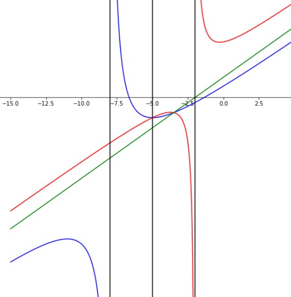
For each range of HH, it is easy to decide the possible range of LL from the graph B.1. If H∈(−∞,−8)H\in(-\infty,-8), it is impossible. If H=−8H=-8, it is impossible. If H∈(−8,−5)H\in(-8,-5), h⁡(H)<L<∞h(H)<L<\infty holds. If H∈(−5,−4)H\in(-5,-4), k⁡(H)<L<−1k(H)<L<-1 holds. If −4<H<−2-4<H<-2, it is impossible. If H=−2H=-2, it is impossible. If H∈(−2,1)H\in(-2,1), it is impossible. If H∈(1,∞)H\in(1,\infty), h⁡(H)<L<k⁡(H)h(H)<L<k(H) holds. Therefore we obtain the following table.

Table B.4: The possible ranges of constants
Range of HH Range of LL Sign of EE
−8<H<−5-8<H<-5 h⁡(H)<L<∞h(H)<L<\infty Negative
−5<H<−4-5<H<-4 k⁡(H)<L<−1k(H)<L<-1 Negative
1<H1<H h⁡(H)<L<k⁡(H)h(H)<L<k(H) Positive
Refer to caption
Figure B.1: The blue, green and red graphs are the graphs of h⁡(H),k⁡(H)h(H),k(H) and f⁡(H)f(H) respectively. The horizontal axis is of HH.

References

  • [1] Kulsrud, Russell M., and Ellen G. Zweibel. ”On the origin of cosmic magnetic fields.” Reports on Progress in Physics 71.4 (2008): 046901.
  • [2] Kramer, D., Stephani, H., MacCallum, M., Herlt, E. (1980). Exact solutions of Einstein’s field equations. Berlin.
  • [3] Ishihara, Hideki, and Satsuki Matsuno. ”Solutions to the Einstein-Maxwell-Current System with Sasakian maifolds.” arXiv preprint arXiv:2012.02432 (2020).
  • [4] Ishihara, Hideki, and Satsuki Matsuno. ”Inhomogeneous generalization of Einstein’s static universe with Sasakian space.” Progress of Theoretical and Experimental Physics 2022.2 (2022): 023E01.
  • [5] Ishihara, Hideki, and Satsuki Matsuno. ”Gödel-type solutions in Einstein–Maxwell–scalar field theories.” Progress of Theoretical and Experimental Physics 2022.1 (2022): 013E02.
  • [6] Dzhunushaliev, Vladimir, and Vladimir Folomeev. ”Dirac/Rarita–Schwinger plus Maxwell theories in ℝ×S3\mathbb{R}\times S^{3} spacetime in the Hopf coordinates.” International Journal of Geometric Methods in Modern Physics 17.13 (2020): 2050197.
  • [7] Cabrerizo, J. L., M. Fernández, and J. S. Gómez. ”The contact magnetic flow in 3D Sasakian manifolds.” Journal of Physics A: Mathematical and Theoretical 42.19 (2009): 195201.
  • [8] Druţa-Romaniuc, S. L., Inoguchi, J. I., Munteanu, M. I., Nistor, A. I. (2015). Magnetic curves in Sasakian manifolds. Journal of Nonlinear Mathematical Physics, 22(3), 428-447.
  • [9] Inoguchi, Jun-ichi, and Marian Ioan Munteanu. ”Magnetic Jacobi fields in three-dimensional Sasakian space forms.” The Journal of Geometric Analysis 32.3 (2022): 96.
  • [10] Kim, Eui Chul, and Thomas Friedrich. ”The Einstein-Dirac equation on Riemannian spin manifolds.” Journal of Geometry and Physics 33.1-2 (2000): 128-172.
  • [11] Friedrich, Thomas. ”Killing spinors in supergravity with 4-fluxes.” Classical and Quantum Gravity 20.21 (2003): 4707.
  • [12] Alekseevsky, D. V., Cortés, V., Devchand, C., Semmelmann, U. (1998). Killing spinors are Killing vector fields in Riemannian supergeometry. Journal of Geometry and Physics, 26(1-2), 37-50.
  • [13] Fujii, Yasunori, and Kengo Yamagishi. ”Killing spinors on spheres and hyperbolic manifolds.” Journal of mathematical physics 27.4 (1986): 979-981.
  • [14] Leitner, Felipe. ”Imaginary Killing spinors in Lorentzian geometry.” Journal of Mathematical Physics 44.10 (2003): 4795-4806.
  • [15] Morris, Michael S., Kip S. Thorne, and Ulvi Yurtsever. ”Wormholes, time machines, and the weak energy condition.” Physical Review Letters 61.13 (1988): 1446.
  • [16] Borde, Arvind, and Alexander Vilenkin. ”Violation of the weak energy condition in inflating spacetimes.” Physical Review D 56.2 (1997): 717.
  • [17] Visser, Matt. ”General relativistic energy conditions: The Hubble expansion in the epoch of galaxy formation.” Physical Review D 56.12 (1997): 7578.
  • [18] Jora, Renata. ”Note about the spin connection in general relativity.” arXiv preprint arXiv:1911.05283 (2019).
  • [19] Boehmer, Christian G., et al. ”Dark spinor models in gravitation and cosmology.” Journal of High Energy Physics 2010.7 (2010): 1-43.
  • [20] Peralta-Salas, Daniel, and Radu Slobodeanu. ”Energy minimizing Beltrami fields on Sasakian 3-manifolds.” International Mathematics Research Notices 2021.9 (2021): 6656-6690.
  • [21] L.I. Nicolaescu, Adiabatic limits of the Seiberg-Witten equations on Seifert manifolds, Comm. Anal. Geom. 6 (1998) 331–392.