Binary synchronization of noise-coupled oscillators

Emergent synchronization has been studied extensively over the last half century, initiated by Kuramoto’s introduction in 1975 Kuramoto 1975; Acebrón et al. 2005 of a paradigmatic model of globally coupled oscillators. Numerous applications exist, from power networks Dörfler and Bullo 2012; Filatrella et al. 2008, to Josephson arrays Watanabe and Strogatz 1993, synchronization of fireflies Ermentrout 1991 and bacterial suspensions Chen et al. 2017. Most modern versions of Kuramoto’s model feature two sources of randomness: the quenched disorder of the randomly chosen intrinsic frequencies, and independent constant-coefficient stochastic noise terms in the dynamics of the oscillators. The first of these models natural variability in populations, the second models inherent stochasticity or unpredictability in the behavior of individual elements. Invariably, both are drivers of global disorder acting counter to the deterministic coupling, raising the coupling strength required to induce synchronization and lowering the coherence of the emergent states.

In other areas of physics situations have been observed in which randomness is in fact a driver global ordering. For example, equilibrium statistical physics possesses many examples of entropically driven ordered states which can be thought of as emerging from purely random interactions, a canonical example being Onsager’s work on nematic fluids Onsager 1949. Recently, there has been some effort to search for similar effects in the dynamics of coupled oscillators. Promising work has included studies considering common noise terms — for example arising from environmental fluctuations — that aid synchronization Pimenova et al. 2016; Ha et al. 2020, but so far the possibility of independent noise driving the emergence of coherent states has been overlooked.

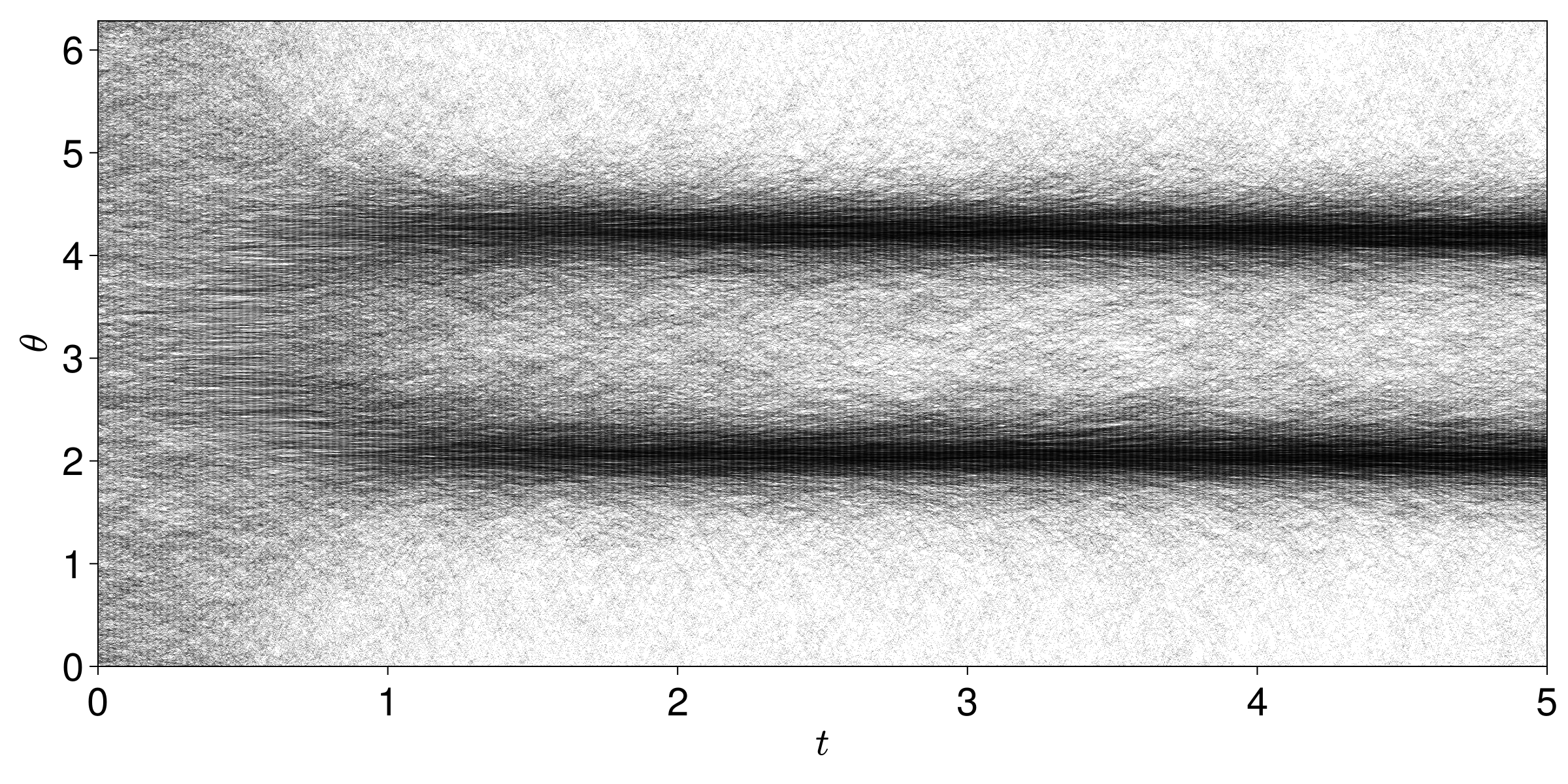
Here, we show that in fact the phase diagram of the Kuramoto model can be replicated in a population of oscillators with purely random forcing. As in the original Kuramoto model the oscillators are only influenced by their phase difference to the others oscillators. Since only the strength of the noise changes, there is no bias on the direction the oscillator moves; remarkably, we show this can be sufficient to induce similar features to traditional Kuramoto coupling models. We further show that the emergent behaviour such as the steady states and individual oscillator movement can be characterised in the order regime, which exhibits a curious phenomenon of binary synchronisation, see Fig. 1. We derive explicit expressions for the steady states and capture the qualitative behaviour of the order parameters with approximate low dimensional dynamics.

We consider a population of $N$ oscillators with phases $\theta_{n}(t)$. Each oscillator has an inherent natural frequency, $\omega_{n}$, sampled from a distribution $g(\omega)$, which should be considered as a source of quenched disorder. There is no deterministic coupling, but each oscillator will be subject to an independent Levy noise term, $\xi_{n}(t)$, whose strength at time $t$ is determined by summing contributions from the rest of the population. Specifically, we write

where $f$ is a function to be chosen, and $\xi_{n}$ is a Levy noise with index $\alpha=2/\beta$. Two cases are of particular interest: if $\beta=1$ then we have Gaussian white noise; if $\beta=2$ then noise terms are Cauchy distributed which facilitates the computation of low-dimensional dynamics Tönjes and Pikovsky 2020.

Our main object of study will be the oscillator density $\rho(\theta,\omega,t)=\frac{1}{Ng(\omega)}\sum_{n}\delta(\theta-\theta_{n}(t))\delta(\omega-\omega_{n})$. Using the shorthand $\left\langle\cdots\right\rangle=\int(\cdots)g(\omega)\;\mathrm{d}\omega$ to denote averaging over the distribution in intrinsic frequencies, the noise strength term in (1) can be written simply as the convolution $\left\langle\rho\ast f\right\rangle$. Applying standard methods Worsfold et al. 2022, one can then take the limit $N\to\infty$ to obtain an integro-differential equation for the oscillator density:

Here we have used the Riesz derivative $\partial^{\alpha}_{|\theta|}$, defined through its action under Fourier transformation Specifically, $\int_{-\pi}^{\pi}e^{-ik\theta}\partial_{|\theta|}^{\alpha}u(\theta)\;\mathrm{d}\theta=-|k|^{\alpha}u_{k}$. Note that in the Gaussian ($\alpha=2$) case, this is simply the diffusion operator. By symmetry, the above equation admits a fixed-point solution that does not vary in phase or time, $\rho_{\circ}\equiv 1/2\pi$, known as the incoherent state. This state may or may not be stable. The phenomenon of synchronisation may broadly be defined as the emergence of one or more peaks in the oscillator phase density which persist over time. An indicator of synchronisation in the system is provided by the complex order parameter

The argument of $z$ gives the average phase, while the modulus describes the level of global coherence; in the incoherent state we have $|z|=0$, whilst full synchronisation implies $|z|=1$.

We begin by examining the dynamics of fluctuations around the incoherent state, studied in detail in Hong 2017. In doing so, we will identify a choice of noise-coupling function $f$ that exactly maps the fluctuations in our system to those of the well-studied noisy Kuramoto model. If $\rho=\rho_{\circ}+\varepsilon\fluc$, where $\varepsilon$ is small, then to leading order (2) yields

Performing the same analysis on the noisy Kuramoto model yields a similar equation for the linear evolution of fluctuations. In fact, if we make the choice $f(\theta)=1-\kappa\cos(\theta)$ then we obtain precisely the same expression for both models:

In Appendix A we give full details of the derivation of this result for both models, and show that this choice for the noise coupling function is the only one for which the statistics fluctuations match.

As a consequence of the equivalence of our noise-coupled oscillator model with the noisy Kuramoto model, the systems have identical phase boundaries for the onset of synchronisation. Following Strogatz and Mirollo Strogatz and Mirollo 1991, we show that for specific choices of the frequency distribution the exact stability boundary for the homogeneous state can be calculated. In Strogatz and Mirollo 1991, it is shown that only the first Fourier mode of the perturbation, $\fluc_{1}(\omega)$ need be considered in the stability analysis. Briefly, this can be seen as the higher modes do not have any contributions from the final term while the first term is diffusive and thus all higher modes decay over time. For the first Fourier mode, we have

Assuming this Fourier mode has an exponential form: $\fluc_{1}(\omega)=\phi(\omega)e^{\eta t}$, then

The average over frequencies, $\left\langle\phi\right\rangle$ is just a constant and so the frequency dependence of $\fluc_{1}$ is

In addition, the average must be self-consistent so that

or equivalently $1=\kappa\left\langle 1/(\eta+1-i\omega)\right\rangle.$ It can be shown that if $g(\omega)$ is a non-increasing function for $\omega>0$, and is symmetric about the origin, then there exists at most one solution for $\eta$ and it is necessarily real (see Strogatz and Mirollo 1991 and Mirollo and Strogatz 1990). Hence, we need only take the real component

as the symmetry in $\omega$ implies that the imaginary component integrates to zero.

Here we only show the result for Lorentz distributed frequencies $g(\omega)=(\gamma^{2}/\pi)[\gamma^{4}+\omega^{2}]^{-1}$, with width $\gamma^{2}$ as it is the focus of subsequent sections. The integrand in (5) can now be separated into partial fractions and integrated with standard results to give

Comparing this to (5), it is clear that $\kappa=1+\gamma^{2}+\eta$. The system is stable if $\eta<0$, which we deduce is satisfied when

which can be seen to match with simulations for various values of $\kappa$ and $\gamma$ in Fig. 3.

With Lorentz distributed intrinsic frequencies, $g(\omega;\gamma)=(\lorentzsig^{2}/\pi)\left[\omega^{2}+\lorentzsig^{4}\right]^{-1}$, the incoherent state is stable for $\kappa<1+\lorentzsig^{2}$, as shown in Fig. 3 (a).

Although the dynamics of our model are indistinguishable from the Kuramoto model in the incoherent phase, the behaviour on the other side of the phase transition is dramatically different. As illustrated in Fig. 1 and Fig. 3 (b-c) simulations of our model exhibit binary synchronisation, with the oscillator population spontaneously dividing into two quasi-coherent phase-locked groups with a consistent separation distance between groups. The remainder of the paper will be devoted to studying this unusual behaviour.

The starting point for all our analysis will be the Fourier representation of the governing equation (2). Writing $\rho_{k}$ for the $k^{\text{th}}$ Fourier mode of $\rho$ (note that $z=2\pi\left\langle\rho_{-1}\right\rangle$), we have

First, we characterize the state of full binary synchronization occurring when $\kappa>1$ if the oscillators all have the same intrinsic frequency. We pick an appropriately chosen rotating reference frame such that the density is symmetric and centred at zero. Then (7) simplifies to

where we can further identify $|z|=2\pi\rho_{1}$. This infinite system of equations can be collapsed by making the ansatz $\rho_{k}=T_{k}(\cos(\Delta))/2\pi$, where $T_{k}$ is the $k^{\text{th}}$ order Chebyshev polynomial of the first kind and $\Delta$ is a non-negative number. Collapsing (8) is possible since the Chebyshev polynomials obey the following rules:

Substituting our ansatz into (8) and writing $T_{k}(\cos\Delta)=T_{k}$ for brevity, this becomes

Thus the ansatz is a solution if $T_{1}=\kappa^{-1/2}$, from which we deduce $\Delta=\arccos(1/\sqrt{\kappa})$.

This solution corresponds to the oscillator phase density condensing to a symmetric pair of Dirac masses with separation $2\Delta$. That is, $\rho(\theta)=\left(\delta(\theta-\Delta)+\delta(\theta+\Delta)\right)/2$. The oscillators become phase locked in these binary positions as the contributions to from each Dirac mass to the convolution term in (2) negatively interfere to precisely cancel each other.

In Fig. 2, while the system approaches the two-peaked steady state, erratic particles diffuse from near one peak to the other. To comprehend better this steady state for identical oscillators, we study the behaviour of a single stray oscillator in the Brownian noise case ($\alpha=2$). Consider the motion of this stray oscillator to be between the two peaks (i.e. $\theta\in[-\Delta,\Delta]$) governed by

The expected time, $\tau(\theta)$, to reach a distance $\epsilon$ from one of the peaks is the solution to $\tau^{\prime\prime}(\theta)=\left[1-\sqrt{\kappa}\cos(\theta)\right]^{-2}$ subject to the boundary conditions $\tau(\Delta-\epsilon)=\tau(\epsilon-\Delta)=0$. Interestingly, the equation above is the same if the oscillators starts at $\Delta<|\theta_{0}|<\pi$ since the increase in noise strength is matched by the larger distance from the peaks. We also observe that, since there is no drift term in Eq. 9, the probability the stray oscillator will reach one peak as opposed to the other is directly proportional to its distance from the peak relative to the other. Explicitly, we have that $p_{\Delta}(\theta_{0})=(\Delta+\theta_{0})/2\Delta$ and $p_{-\Delta}(\theta_{0})=1-p_{\Delta}(\theta_{0})$ where $p_{\pm\Delta}(\theta_{0})$ are the probabilities the oscillator will reach $\theta=\pm\Delta$ eventually (see Gardiner 2009 and Appendix C).

Studying an individual oscillator gives intuition for why the two-peaked state is stable for $\kappa>1$. Assume all particles are perturbed by a small amount, $\vartheta_{i}$. If the perturbation is small enough so that $\sqrt{\kappa^{\prime}}=\kappa|z|>1$ still holds, each oscillator still has a solution to $\dot{\theta}=[1-\sqrt{\kappa^{\prime}}\cos(\theta)]\xi(t)$ and the probability that it will return to its closest peak can be approximated by $p_{\Delta}(\Delta-\vartheta_{i})$. Hence, at least close to this solution, it appears to be stochastically asymptotically stable Mao 2011. Due to the irregularity of the two-peak solution, formally showing stability from the macroscopic scale would be a more involved task, which we leave for future work.

We broaden our investigation now to address the more general case of heterogeneous intrinsic frequencies. In the last two decades, great strides have been made in describing the dynamics of Kuramoto-like systems in terms of simple equations for the order parameters. Starting with the Watanabe-Strogatz variables Watanabe and Strogatz 1993, it was shown that a suitable transformation on the oscillator phase to a homogeneous, stationary phase results in just three equations needed to describe the full dynamics of the system of $N$ particles Marvel et al. 2009. Ott and Antonsen Ott and Antonsen 2008 subsequently derived similar equations for the order parameters.

These equations connect the nonequilibrium transition from the incoherent state to the synchronised state. Incorporating intrinsic noise has presented another challenge as the Ott-Antonsen manifold no longer holds when the oscillator phases have additive Brownian noise Tyulkina et al. 2018a. When Cauchy noise is included instead, it has been shown to give equivalent low dimensional dynamics as systems with Lorentz distributed frequencies Tanaka 2020. Exact low dimensional expressions for the steady states of models more complex coupling has also been achieved with Cauchy noise Tönjes and Pikovsky 2020. We use a similar approach here to identify the non-trivial steady state of the model presented above.

When the incoherent state is unstable, the distribution evolves towards a bimodal distribution (see Fig. 1) which is surprisingly distinct to the unimodal distribution seen in the Kuramoto model. As with the majority of Kuramoto-based models, we examine the case where the oscillator frequencies are Lorentz distributed. This enables the bimodal distribution at the steady state of (7) to be solved exactly.

In steady state, the mode-coupling equation (7) is of a class studied by Tönjes and Pikovsky Tanaka 2020, who proposed to seek solutions of the form

where $\lambda_{1},\lambda_{2}$ are complex parameters lying in the unit disc, and $c_{1},c_{2}$ are normalization coefficients summing to $1/2\pi$. Explicitly,

and $c_{2}(\omega)=1/2\pi-c_{1}(\omega)$. In real (phase) space, this ansatz posits that the density of oscillators with a given frequency has the form of the product of two wrapped Cauchy distributions, also known as a Kato-Jones distribution (cf. Kato and Jones 2013; Tanaka 2020). Specifically, this distribution can be written as

where $M$ is a normalisation constant given by

and we have omitted the dependence of $\omega$ on $\lambda_{1},\lambda_{2}$. In this distribution, the arguments of the complex parameters $\lambda_{1}$ and $\lambda_{2}$ determine the positions of the two peaks, while the moduli determine the coherence and relative weighting of the peaks.

Applying (10) to (7) reveals an equation that must be satisfied by each of these complex parameters. Firstly, for $k\geqslant 1$

If the argument in the curly brackets is zero for each of $n=1,2$ then dividing through by $k\lambda_{n}^{k}$, we obtain

Recalling that $z=2\pi\left\langle\rho_{-1}\right\rangle$, we see that this equation must be solved self-consistently with $z$ determined as a function of $\lambda_{1,2}$. Here we appeal to the remarkable result of Ott and Antonsen Ott and Antonsen 2008, that when the intrinsic frequencies are chosen from a Lorentz distribution, disorder averaging can be replaced by evaluation at a particular complex frequency. Specifically, if $g(\omega)=\left[(\omega-i\lorentzsig^{2})^{-1}-(\omega+i\lorentzsig^{2})^{-1}\right]/2\pi i$ then $\left\langle\rho_{k}\right\rangle=\rho_{k}(-i\gamma^{2})$. The symmetry of $g$ implies that we may choose a frame of reference in which the disorder-averaged stationary distribution $\left\langle\rho\right\rangle$ is also symmetric, implying that $\left\langle\lambda_{1}\right\rangle=\left\langle\overline{\lambda_{2}}\right\rangle=\lambda$. The frequency-averaged distribution can thus be written as

Moreover, the frequency averaged Fourier modes, $\left\langle\rho_{k}\right\rangle=\left\langle c_{1}\right\rangle\left\langle\lambda\right\rangle^{k}+\left\langle c_{2}\right\rangle\left\langle\overline{\lambda}\right\rangle^{k}$, now have normalisation constants given by

or, after some manipulation

from which we see that $\left\langle c_{1}\right\rangle=\left\langle\overline{c_{2}}\right\rangle$ recalling that $\left\langle c_{2}\right\rangle=1/2\pi-\left\langle c_{1}\right\rangle$. This is also apparent as we require $\left\langle\rho_{k}\right\rangle=\left\langle c_{1}\right\rangle\lambda^{k}+\left\langle c_{2}\right\rangle\bar{\lambda}^{k}$ to be real which is only satisfied for all $k$ if $\left\langle c_{1}\right\rangle=\left\langle\overline{c_{2}}\right\rangle$. Returning to the order parameter, $z=2\pi(\left\langle c_{1}\right\rangle\lambda+\left\langle c_{2}\right\rangle\bar{\lambda})$, after some simplification we can compactly express this as

Consequently, (15) reduces (12) to the algebraic equation

Of the possible roots within the unit disc (accounting for rotation and reflection symmetry) we pick the one in the top right quadrant and write it as $\lambda=|\lambda|e^{i\Delta}$. The solution can then be explicitly stated

This solution only exists for $\kappa>\lorentzsig^{2}+1$, matching the stability condition for the incoherent state, and in the limit $\gamma\to 0$ it recovers the Dirac mass pair solution obtained above. The argument of $\lambda$ is the separation between the peaks in $\rho$, while the modulus controls their coherence. For small values of $\gamma$ and large values of $\kappa$, the peaks are sharp whereas they become less pronounced when $\gamma$ is small and as $\kappa\to\gamma^{2}+1$ as can be seen in Fig. 3. From this solution we also obtain a closed expression for the averaged coherence order parameter: $|z|=2|\lambda|\cos(\Delta)/(|\lambda|^{2}+1)=\sqrt{(\kappa-\lorentzsig^{2}-1)/\kappa(\kappa-1)}$.

We now extend the method applied above beyond the stationary states to deduce approximate low-dimensional dynamics for the evolution of the disorder averaged oscillator phase density for Cauchy noise. Applying the disorder average to (7) in the case $\alpha=1$, we obtain

Similarly, the disorder average of the Tönjes-Pikovsky ansatz (10) is simply $\left\langle\rho_{k}\right\rangle=c\lambda^{k}+\overline{c\lambda^{k}}$. This is consistent with (18) if $c$ is assumed constant, and if

This equation describes the approximate low dimensional dynamics of the order parameter $\lambda$. Unlike the Ott-Antonsen manifold for the Kuramoto model with Cauchy noise and Lorentz intrinsic frequencies, this is not an exact mapping; the coefficient $c$ actually has a non-constant imaginary part, which was ignored in the derivation of (19). Nonetheless, we find it provides a good qualitative description of the evolution of the system in simulation experiments.

To test the predictive power of our approximate low dimensional dynamics, we prepare a finite sample system in a state consistent with the Tönjes-Pikovsky ansatz and forward integrate. A time series for $\lambda$ can be inferred by fitting the empirical distribution of oscillator phase to the Kato-Jones distribution in (13). Full details of how to correctly prepare the samples are provided in Appendix B. Figure 4 shows the complex flow field described by (19), overlayed with simulation results for various initial values of $\lambda$. We see that the approximate low dimensional dynamics represent well the trajectory of the order parameter as it evolves towards the steady state.

To summarise, we have sought to find a model of synchronization arising from coupling purely in the noise strength on each oscillator. This model differs from almost all previous models of synchronization as the tendency towards synchrony is completely intrinsic to the system, with each oscillator acting under independent noise. In contrast, the existing literature focuses on deterministic coupling or random coupling through external or common noise to each oscillator. The specific choice made reproduces the exact stability condition about the incoherent state for the noisy Kuramoto model with a general frequency distribution Strogatz and Mirollo 1991. For the other stationary state, comparisons can be made to systems with multi-harmonic, deterministic coupling Tanaka 2020. We applied the approaches developed for such systems to this model, which enabled us to characterise the binary synchronised steady state in terms of a Kato-Jones distribution. While not being exact, this description was also useful in describing the general dynamics of the system in terms of the order parameter $\lambda$. It remains to be seen if an exact description of the low dimensional manifold can be found. This has also been a challenge for more traditional Kuramoto models with noise. Recent developments have shown that the Ott-Antonsen ansatz can be generalised to a larger family of invariant manifolds Tyulkina et al. 2018b and so it is possible a similar approach could be taken for the system present in this article.

Acknowledgements. JW supported by the EPSRC: EP/S022945/1.

References

- Kuramoto (1975) Y. Kuramoto, Self-entrainment of a population of coupled non-linear oscillators, in International Symposium on Mathematical Problems in Theoretical Physics, edited by H. Araki (Springer Berlin Heidelberg, Berlin, Heidelberg, 1975) pp. 420–422.
- Acebrón et al. (2005) J. A. Acebrón, L. L. Bonilla, C. J. Pérez Vicente, F. Ritort, and R. Spigler, The Kuramoto model: A simple paradigm for synchronization phenomena, Rev. Mod. Phys. 77, 137 (2005).
- Dörfler and Bullo (2012) F. Dörfler and F. Bullo, Synchronization and transient stability in power networks and nonuniform Kuramoto oscillators, SIAM Journal on Control and Optimization 50, 1616 (2012).
- Filatrella et al. (2008) G. Filatrella, A. H. Nielsen, and N. F. Pedersen, Analysis of a power grid using a Kuramoto-like model, The European Physical Journal B 61, 485 (2008).
- Watanabe and Strogatz (1993) S. Watanabe and S. H. Strogatz, Integrability of a globally coupled oscillator array, Phys. Rev. Lett. 70, 2391 (1993).
- Ermentrout (1991) B. Ermentrout, An adaptive model for synchrony in the firefly pteroptyx malaccae, Journal of Mathematical Biology 29, 571 (1991).
- Chen et al. (2017) C. Chen, S. Liu, X.-q. Shi, H. Chaté, and Y. Wu, Weak synchronization and large-scale collective oscillation in dense bacterial suspensions, Nature 542, 210 (2017).
- Onsager (1949) L. Onsager, The effects of shape on the interaction of colloidal particles, Annals of the New York Academy of Sciences 51, 627 (1949).
- Pimenova et al. (2016) A. V. Pimenova, D. S. Goldobin, M. Rosenblum, and A. Pikovsky, Interplay of coupling and common noise at the transition to synchrony in oscillator populations, Scientific Reports 6, 38518 (2016).
- Ha et al. (2020) S.-Y. Ha, D. Ko, C. Min, and X. Zhang, Emergent collective behaviors of stochastic kuramoto oscillators, Discrete and Continuous Dynamical Systems - B 25, 1059 (2020).
- Tönjes and Pikovsky (2020) R. Tönjes and A. Pikovsky, Low-dimensional description for ensembles of identical phase oscillators subject to Cauchy noise, Phys. Rev. E 102, 052315 (2020).
- Worsfold et al. (2022) J. Worsfold, T. Rogers, and P. Milewski, Density fluctuations in stochastic kinematic flows, arXiv preprint arXiv:2204.02926 (2022).
- Hong (2017) H. Hong, Finite-size scaling in the system of coupled oscillators with heterogeneity in coupling strength, Phys. Rev. E 96, 012213 (2017).
- Strogatz and Mirollo (1991) S. H. Strogatz and R. E. Mirollo, Stability of incoherence in a population of coupled oscillators, Journal of Statistical Physics 63, 613 (1991).
- Mirollo and Strogatz (1990) R. E. Mirollo and S. H. Strogatz, Amplitude death in an array of limit-cycle oscillators, Journal of Statistical Physics 60, 245 (1990).
- Gardiner (2009) C. Gardiner, Stochastic methods, Vol. 4 (Springer Berlin, 2009).
- Mao (2011) X. Mao, 4 - stability of stochastic differential equations, in Stochastic Differential Equations and Applications (Second Edition), edited by X. Mao (Woodhead Publishing, 2011) second edition ed., pp. 107–146.
- Marvel et al. (2009) S. A. Marvel, R. E. Mirollo, and S. H. Strogatz, Identical phase oscillators with global sinusoidal coupling evolve by möbius group action, Chaos: An Interdisciplinary Journal of Nonlinear Science 19, 043104 (2009).
- Ott and Antonsen (2008) E. Ott and T. M. Antonsen, Low dimensional behavior of large systems of globally coupled oscillators, Chaos: An Interdisciplinary Journal of Nonlinear Science 18, 037113 (2008).
- Tyulkina et al. (2018a) I. V. Tyulkina, D. S. Goldobin, L. S. Klimenko, and A. Pikovsky, Dynamics of noisy oscillator populations beyond the Ott-Antonsen ansatz, Physical review letters 120, 264101 (2018a).
- Tanaka (2020) T. Tanaka, Low-dimensional dynamics of phase oscillators driven by Cauchy noise, Phys. Rev. E 102, 042220 (2020).
- Kato and Jones (2013) S. Kato and M. Jones, An extended family of circular distributions related to wrapped Cauchy distributions via Brownian motion, Bernoulli 19, 154 (2013).
- Tyulkina et al. (2018b) I. V. Tyulkina, D. S. Goldobin, L. S. Klimenko, and A. Pikovsky, Dynamics of noisy oscillator populations beyond the Ott-Antonsen ansatz, Phys. Rev. Lett. 120, 264101 (2018b).
- Schelling (1971) T. C. Schelling, Dynamic models of segregation, The Journal of Mathematical Sociology 1, 143 (1971).
Appendix A Stability of the incoherent state
In terms of the density of oscillators, , the general system in the main text is