IINTRODUCTION

Two dimensional penetrative phototactic bioconvection with periodic sidewalls
M. K. Panda¹¹¹ 1 Corresponding author; e-mail:mkpanda@iiitdmj.ac.in

¹ Department of Mathematics, PDPM Indian Institute of Information Technology Design and Manufacturing, Jabalpur 482005, India

Abstract

Light gradient can allow many motile photosynthetic microorganisms to bias their motion towards moderate light (positive phototaxis) or away from intense light (negative phototaxis). The proposed work presents the penetrative phototactic bioconvection in a non-scattering algal suspension. The suspension is confined by a stress-free top boundary, and rigid bottom and periodic lateral boundaries. The resulting bioconvective patterns of the problem strongly resemble to that of a spatially extended domain in the same vicinity. The bioconvection solution appears in the form of a two-rolls pattern (or any even number of rolls) due to the periodic lateral boundaries.

I INTRODUCTION

Bioconvection is recognized as the convective flows generated by the upward swimming motile microorganisms and it arises due to the differences in density between them and the fluid in their local environment [1, 2]. Usually, it appears spontaneously in biological suspensions and identified by emergent flow patterns. When the microorganisms are of non-motile type, the flow patterns also do not appear. It is not difficult to find out examples of pattern formation where the microorganisms do not swim upward and are not heavier than the surrounding fluid [1]. The swimming microorganisms found to bioconvect in biological suspensions are mostly bacteria, algae, and protozoa and so on. The response of microorganisms to external gradients or passive forces, which allow them to orient in particular directions in their environment is called taxes. For instance, gravitaxis represents a motion induced along the direction of gravity for a microorganism with asymmetry mass distribution. In addition, if orientation of a microorganism is affected by a local shear due to fluid flow then the induced motion is named as gyrotaxis. Phototaxis is a mechanism by which a microorganism detects light gradients. This article accounts phototaxis only.

Laboratory experiments have shown that illumination can affect the bioconvection patterns [3, 4, 5]. For instance, the patterns in biological suspensions may be destroyed or their formation may be blocked via intense light. The reasons behind the changes in bioconvective flow patterns via light intensity may be as follows: The motile phototactic microorganisms detect light gradients and they exhibit positive phototaxis (i.e. $I<I_{c}$ ) and negative phototaxis (i.e. $I>I_{c}$ ). Thus, they select an optimal location across the suspension where $I\approx I_{c}$ . The second reason is as follows. The algae absorb the light incident on them and it decreases along the incident direction of light. If the algal suspension is dilute and non-scattering, then the Lambert–Beer law gives the governing equation for light intensity $I(x,y,z)$ as [6] i.e.

I(x,y,z)=I_{t}\,\exp{\left(\alpha\int_{\gamma}n\,ds\right)}.

(1)

Here $I_{t}$ is the magnitude of vertical collimated solar flux, $\alpha$ is the absorption coefficient, $n$ is the cell concentration and $\gamma$ is a straight line segment connecting algae and the light source. If $<{\boldsymbol{p}}>$ denotes the average swimming direction of cells in a small volume, then [7]

<{\boldsymbol{p}}>=M(I)\hat{\boldsymbol{z}},

(2)

where the swimming direction of a cell is defined by ${\boldsymbol{p}},$ $\hat{\boldsymbol{z}}$ is the unit vector directed vertically upwards. $M(I)$ is the photoresponse curve such that

M(I)\left\{\begin{array}[]{c }\geq 0\quad\mbox{if}\quad I\leq I_{c},\\ <0\quad\mbox{if}\quad I>I_{c}.\end{array}\right.

(3)

Here ${\boldsymbol{W}_{c}}=W_{c}<{\boldsymbol{p}}>$ represents the mean swimming velocity, where $W_{c}$ is the ensemble-average swimming speed.

Consider a biological suspension with an vertical collimated solar flux as the illuminating source. The equilibrium state for such a finte-depth suspension is the resultant between phototaxis with cell diffusion. As a result, a sublayer of algae is formed across the suspension as a function of intensity of light. The unstable zone is defined as the region below the sublayer and the region above it is defined as gravitationally unstable zone. The motion induced by convection from the unstable zone penetrates the upper stable zone [8].

Many motile algae are strongly phototactic as they need to photosynthesize in order to survive. Thus, realistic and reliable models of their behaviour should include phototaxis. Phototaxis and the corresponding bioconvection also have important applications in biofuel, biohydrogen production, and biofluid dynamics research [10, 9, 11].

Gyrotactic, gravitactic and chemotactic bioconvection have been explored extensively via numerical simulation [2, 12]. However, there has not been much numerical simulation on phototactic bioconvection available till date except few [10, 7, 13]. Two-dimensional phototactic bioconvection in a layer confined by a rigid bottom boundary, stress-free top and lateral boundaries was investigated by Ghorai and Hill [7] in the nonlinear regime. They used the phototaxis model proposed by Vincent and Hill [6]. Panda and Ghorai [10] simulated numerically phototactic bioconvection in an isotropic scattering suspension using the phototaxis model proposed by Ghorai et al. [14]. Two-dimensional phototactic bioconvection was simulated numerically by Panda and Singh [13] in a layer confined by a stress-free top boundary, rigid bottom and lateral boundaries. Bioconvection in small domains with periodic sidewalls has been hitherto carried out as a model of a spatially extended system and the proposed work investigates penetrative phototactic bioconvection on the same vicinity.

The manuscript is organized as follows: In Sec. II, the problem is converted into mathematical form. In Sec. III, the numerical procedure is proposed. In Sec. IV, the numerical results are presented. Finally, conclusions are drawn in Section VII.

II Mathematical formulation

II.1 Geometry of the problem

The geometry consists of a chamber with width $L$ and height $H$ referred to Cartesian coordinates $\left(x,z\right)$ with the $z$ -axis pointing vertically upwards. Thus, the flow is confined in the $xz$ -plane and is independent of the $y$ coordinate [see Fig. 1].

Refer to caption — Fig. 1: Geometry of the problem.

II.2 Governing equations

We employ a continuum approach similar to the previous models on bioconvection [6, 1] and each cell has a volume $\vartheta$ and density $\rho+\Delta\rho$ , where $\Delta\rho\ll\rho$ ad $\rho$ is the constant density of the water. Let ${\boldsymbol{u}}=u\hat{\boldsymbol{x}}+w\hat{\boldsymbol{z}}$ and $n$ denote the average velocity and cell concentration over an elemental volume, where $\hat{\boldsymbol{x}}$ and $\hat{\boldsymbol{z}}$ are unit vectors along $x$ and $z$ axes. Assume that the suspension is incompressible and the flow is restricted to two dimensions only. Introducing stream function $\psi$ and vorticity $\zeta$ , we get

{\boldsymbol{u}}=\left(\frac{\partial{\psi}}{\partial{z}},0,-\frac{\partial{\psi}}{\partial{x}}\right),\quad\zeta=-\nabla^{2}\psi.

(4)

The momentum equation under the Boussinesq approximation leads to the vorticity equation

\frac{\partial{\zeta}}{\partial{t}}+\boldsymbol{\nabla}\boldsymbol{\cdot}\left(\zeta{\boldsymbol{u}}\right)=\nu\nabla^{2}\zeta-\frac{\Delta\rho g\vartheta}{\rho}\,\frac{\partial{n}}{\partial{x}}.

(5)

The conservation equation for microorganisms is given by

\frac{\partial{n}}{\partial{t}}=-{\boldsymbol{\nabla}}\cdot{\boldsymbol{J}},

(6)

where the flux of the cells is

{\boldsymbol{J}}=n{\boldsymbol{u}}+nW_{c}<{\boldsymbol{p}}>-D{\boldsymbol{\nabla}}{n}.

(7)

Here the first term, second term and third term represent the flux induced by advection of bulk fluid flow, average swimming of cells and random motion of cells respectively. We assume ${\textrm{\bf D}}=D{\textrm{\bf I}}.$ For a uniformly illuminated suspension via a vertical collimated solar flux as considered by Ghorai and Hill [7], the Eq. (1) for light intensity becomes

I(x,z)=I_{t}\,\exp{\left[-\alpha\,\int_{z}^{H}n(x,z)dz\right]}.

(8)

II.3 Boundary conditions

We impose rigid, no-slip boundary condition on $z=0$ and periodic boundary condition at $x=0,L$ . We require that both the normal velocity and tangential stress vanish on $z=H$ . Also there is no flux of cells through the walls. Thus the boundary conditions are

	$\displaystyle\psi=0\quad\mbox{and\ }\quad{\boldsymbol{J}}\cdot{\hat{\boldsymbol{z}}}=0\quad\mbox{at\ }\quad z=0,H,$		(9)
	$\displaystyle\frac{\partial{\psi}}{\partial{z}}=0\quad\mbox{at}\quad z=0\quad\mbox{and}\quad\zeta=0\quad\mbox{at}\quad z=H,$		(10)
	$\displaystyle\psi=0,~\zeta=0\quad\mbox{and}\quad{\boldsymbol{J}}\cdot{\hat{\boldsymbol{x}}=0\quad\mbox{at}\quad}x=0,L,$		(11)

and a periodic boundary condition with period $L$ is imposed in the $x-$ direction (i.e. $\psi{(0,z)}=\psi{(L,z)}$ ).

II.4 Scaling of the equations

Length is scaled on the depth $H$ , velocity on $D/H$ , time on the diffusive scale ${H^{2}/D}$ , and the cell concentration on the mean cell concentration $\overline{n}$ . Now, the governing system for bioconvection in terms of stream function $\psi$ and vorticity $\zeta$ , is recasted as:

\zeta=-\nabla^{2}\psi,

(12)

\frac{\partial{\zeta}}{\partial{t}}+{\boldsymbol{\nabla}}\cdot{\left(\zeta{\boldsymbol{u}}\right)}=S_{c}\nabla^{2}{\zeta}-S_{c}R\frac{\partial{n}}{\partial{x}},

(13)

and

\frac{\partial{n}}{\partial{t}}=-{\boldsymbol{\nabla}}\cdot{\boldsymbol{J}},

(14)

where the flux of the cells is

{\boldsymbol{J}}=n{\boldsymbol{u}}+nV_{c}<{\boldsymbol{p}}>-{\boldsymbol{\nabla}}{n}.

(15)

Here $S_{c}=\nu/D$ is the Schmidt number, $V_{c}=W_{c}H/D$ is the scaled swimming speed, and $R={\overline{n}v\Delta{\rho{g}H^{3}}}/{\rho{\nu{D}}}$ is the Rayleigh number. Also $<{\boldsymbol{p}}>=M(I)\hat{\boldsymbol{z}}$ with $I$ given by

I(x,z)=I_{t}\exp\left[-\kappa{\int\limits_{z}^{1}n(x,z)dz}\right],

(16)

where $\kappa=\alpha{\overline{n}H}$ is the nondimensional extinction (absorption) coefficient. The phototaxis functions is generated by superimposing the sine functions:

M\left(I\right)=0.8\sin{\left[\frac{3\pi}{2}\chi{\left(I\right)}\right]}-0.1\sin{\left[\frac{\pi}{2}\chi{\left(I\right)}\right]},

(17)

where $\chi{\left(I\right)}=I\exp{\left[\beta\left(I-1\right)\right]}$ . Eqs. (12)–(14) are solved in the region $0\leq{x\leq{\lambda}}$ and $0\leq{z\leq{1}}$ , where $\lambda=L/H$ is the normalized width of the domain.

We impose rigid, no-slip boundary condition on $z=0$ and periodic boundary condition at $x=0,\lambda$ (i.e. $\psi{(0,z)}=\psi{(\lambda,z)}$ ). We require that both the normal velocity and tangential stress vanish on $z=1$ . Also there is no flux of cells through the walls. Thus the boundary conditions are

	$\displaystyle\psi=0\quad\mbox{and\ }\quad{\boldsymbol{J}}\cdot{\hat{\boldsymbol{z}}}=0\quad\mbox{at\ }\quad z=0,1,$		(18)
	$\displaystyle\frac{\partial{\psi}}{\partial{z}}=0\quad\mbox{at}\quad z=0\quad\mbox{and}\quad\zeta=0\quad\mbox{at}\quad z=1,$		(19)
	$\displaystyle\psi=0,~\zeta=0\quad\mbox{and}\quad{\boldsymbol{J}}\cdot{\hat{\boldsymbol{x}}=0\quad\mbox{at}\quad}x=0,\lambda.$		(20)

We choose $\lambda=\lambda_{c}$ to compute the solution in the full convection cell and the initial conditions are $\psi=0,~\zeta=0,~n=1+\epsilon{\cos\left(\pi{x}/\lambda\right)},\quad\mbox{where}\quad\epsilon=10^{-5}$ .

III The numerical procedure

The governing Eqs. (12)–(14) with appropriate boundary conditions are solved using a conservative finite-difference scheme via stream function-vorticity formulation [7, 15] and the corresponding critical values at the onset of bioconvection are computed in the $(k,R)$ –plane by linear stability theory as similar to Panda and Singh [13].

IV Results

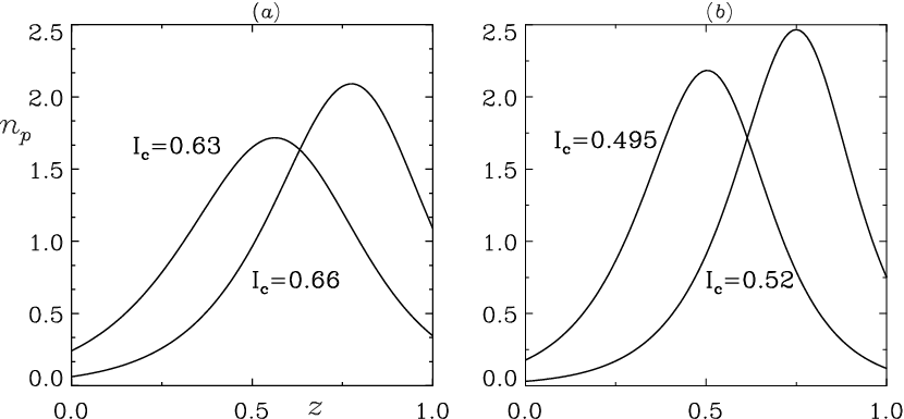
The representative parameter values are $V_{c}=10,15,20$ and $\kappa=0.5,1.0$ respectively. The value of critical intensity $I_{c}$ is selected so that the sublayer where the cells aggregate at equilibrium state lies either around $z=3/4$ or $z=1/2$ of the suspension (see Fig. 2). In this investigation, the Rayleigh number is varied such that $1.5R_{c}\leq R\leq 100R_{c}$ and some steady convection solutions of the proposed study are presented here [see Figs. 3–6].

V $V_{c}=10$

V.1 Extinction coefficient $\kappa=0.5$

We start with the case, when $V_{c}=10,$ $\kappa=0.5,$ and $I_{c}=0.66.$ In this case, the sublayer via equilibrium state is located at around three-quarter height of the domain [see Fig. 2(a)]. Fig. 3 shows the bioconvective solutions for Rayleigh number $R$ such that $1.5R_{c}\leq R\leq 30R_{c}.$ For $R=1.5R_{c},$ a steady state two convection cells solution is observed. When $R$ is increased to $5R_{c}$ the two convection cells solution is replaced by a four convection cells solution and it persists upto $R=20R_{c}.$ When $R$ is increased to $30R_{c},$ small counter rotating cells appear above the convection cells. If $R$ is increased further, the bioconvective solution becomes periodic.

Next, we consider the case when $V_{c}=10,$ $\kappa=1,$ and $I_{c}=0.63.$ In this case, the sublayer via equilibrium state is located at around mid-height of the domain [see Fig. 2(a)]. Fig. 4 shows the bioconvective solutions for Rayleigh number $R$ such that $1.5R_{c}\leq R\leq 40R_{c}.$ For $R=1.5R_{c},$ a steady state two convection cells solution is observed. When $R$ is increased to $5R_{c}$ the two convection cells solution is replaced by a four convection cells solution and small counter rotating cells appear above the convection cells. At $R=20R_{c},$ the small counter rotating cells which appear above the convection cells grow in height and the trend continues when $R$ is increased to $40R_{c}.$ If $R$ is increased further, the bioconvective solution becomes periodic.

V.2 Extinction coefficient $\kappa=1$

Here start with the case, when $V_{c}=10,$ $\kappa=1,$ and $I_{c}=0.52.$ In this case, the sublayer via equilibrium state is located at around three-quarter height of the domain [see Fig. 2(b)]. Fig. 5 shows the bioconvective solutions for Rayleigh number $R$ such that $1.5R_{c}\leq R\leq 70R_{c}.$ For $R=1.5R_{c},$ a steady state two convection cells solution is observed. When $R$ is increased to $10R_{c}$ the two convection cells solution is replaced by a four convection cells solution and small counter rotating cells appear above the convection cells. The same trend continues when $R$ is increased upto $70R_{c},$ small counter rotating cells which appear above the convection cells grow in height. If $R$ is increased further, the bioconvective solution becomes periodic.

Next, we consider the case when $V_{c}=10,$ $\kappa=1,$ and $I_{c}=0.495.$ In this case, the sublayer via equilibrium state is located at around mid-height of the domain [see Fig. 2(b)]. Fig. 6 shows the bioconvective solutions for Rayleigh number $R$ such that $1.5R_{c}\leq R\leq 30R_{c}.$ For $R=1.5R_{c},$ a steady state two convection cells solution is observed. When $R$ is increased to $5R_{c}$ the two convection cells solution is replaced by a four convection cells solution and small counter rotating cells appear above the convection cells. At $R=20R_{c},$ the small counter rotating cells which appear above the convection cells grow in height and the trend continues when $R$ is increased to $30R_{c}.$ If $R$ is increased further, the bioconvective solution becomes periodic.

VI $V_{c}=15$ and $V_{c}=20$

We have also found the bioconvective solutions for $V_{c}=15$ and $V_{c}=20$ too and the solutions are qualitatively similar to those of $V_{c}=10.$

VII CONCLUSIONS

In this study, two-dimensional phototactic bioconvection in a suspension of non-scattering algae is simulated numerically. Since small domains with periodic sidewalls can be considered as a model of a spatially extended system, the suspension is confined by a stress-free top boundary, and rigid bottom and periodic lateral boundaries. The intensity of light via critical intensity is adjusted so that the sublayer at the equilibrium state lies either at the midheight or three-quarter height of the domain. The non-scattering model for phototaxis proposed by Vincent and Hill [6] is employed in this study and the governing bioconvective system is solved using a conservative finite-difference scheme via stream function-vorticity formulation.

The discrete parameters taken in this study are $V_{c}=10,15,20$ and $\kappa=0.5,1.0$ respectively and the Rayleigh number $R$ is varied such that $1.5R_{c}\leq R\leq 100R_{c}$ . The conclusions drawn from the present study are as follows. The bioconvection solutions always appear in the form of a two-rolls pattern (or any even number of rolls) due to presence of periodic lateral boundaries. The number of convection cells increases as the Rayleigh number increases. The symmetry with respect to the midvertical line in bioconvection cells slution does not persist. Also, the weak counter rotating cells appear on top of the main convection cells and grow in size as the Rayleigh number increases.

To test this proposed theoretical model with the available experimental results, we refer the quantitative study by Williams and Bees [11] and it is in agreement with the experimental results via appearance of multitude of plumes with the increment in Rayleigh number. Penetrative phototactic bioconvection in a non-scattering suspension is in the process of extension to three dimensions since bioconvection is intrinsically a three-dimensional phenomena.

Acknowledgements

The corresponding author gratefully acknowledges the COUNCIL OF SCIENTIFIC AND INDUSTRIAL RESEARCH (CSIR), Government of India for the financial support via the Extramural Research Grant (Grant No. 25(0295)/19/EMR-II).

References

[1] T.J. Pedley and J.O. Kessler, “Hydrodynamic phenomena in suspensions of swimming microorganisms," Ann. Rev. Fluid Mech. 24, 313 (1992).
[2] N. A. Hill and T. J. Pedley, “Bioconvection," Fluid Dyn. Res. 37, 1 (2005).
[3] H. Wager, “On the effect of gravity upon the movements and aggregation of Euglena viridis. Ehrb., and other microorganisms," Phil. Trans. R. Soc. London, Ser. B 201, 333 (1911).
[4] J.O. Kessler, “Co-operative and concentrative phenomena of swimming microorganisms," Contemp. Phys. 26, 147 (1985).
[5] R.V. Vincent, “Mathematical modelling of phototaxis in motile microorganisms," Ph.D. thesis, University of Leeds, 1995.
[6] R.V. Vincent and N.A. Hill, “Bioconvection in a suspension of phototactic algae," J. Fluid Mech. 327, 343 (1996).
[7] S. Ghorai and N.A. Hill, “ Penetrative phototactic bioconvection," Phys. Fluids 17, 074101 (2005).
[8] B. Straughan, Mathematical aspects of penetrative convection, (Longman Scientific & Technical, 1993).
[9] T. Ishikawa, “Suspension biomechanics of swimming microbes," J. R. Soc. interface 6, 815 (2009).
[10] M. K. Panda and S. Ghorai, “Penetrative phototactic bioconvection in an isotropic scattering suspension," Phys. Fluids, 25 (071902), 1 (2013).
[11] C. R. Williams and M. A. Bees, “A tale of three taxes: photo-gyro-gravitactic bioconvection," The Journal of Experimental Biology, 214, 2398 (2011).
[12] H. G. Lee and J. Kim,“Numerical investigation of falling bacterial plumes caused by bioconvection in a three-dimensional chamber," European Journal of Mechanics B/Fluids, 52, 120 (2015).
[13] M. K. Panda and R. Singh, “Penetrative phototactic bioconvection in a two-dimensional non-scattering suspension," Phys. Fluids, 28, 054105 (2016).
[14] S. Ghorai, M. K. Panda and N. A. Hill, “Bioconvection in a suspension of isotropically scattering phototactic algae," Phys. Fluids 22, 071901 (2010).
[15] S. Ghorai, “Bioconvection and plumes," Ph.D. thesis, University of Leeds, (1997).