Ensemble Gaussian Processes
for Adaptive Autonomous Driving on Multi-friction Surfaces

To calculate the prediction of the ensembled model, we need to first calculate the vector of weights

Let $\hat{y}^{n}$ be the prediction of the $n^{th}$ GP $\hat{y}^{n}=f_{\mu}^{n}(x^{i})$, where $x^{i}$ is the input to the GP. Let $y$ be the true value of the output. Given the history of the length $K$ of the output-input pairs $[(y_{k-1},x^{i}_{k-1}),\dots,(y_{k-K},x^{i}_{k-K})]$ our goal is to calculate the combination of models that provide the best representation over the history. We can formulate this problem as the following optimization program:

where $Y$ is the vector of true output values

$F$ is a matrix of predictions from all of the models over the whole history

and $\alpha$ is a regularization parameter that minimizes the distance between the previous estimate of the weights $w_{k-1}$ and the new weights.

In this section, we present the system identification strategy. We consider a vehicle with states:

where $p^{x}$ and $p^{y}$ are the position in Cartesian coordinates, $\psi$ is the orientation, $v_{x}$ and $v_{y}$ are the longitudinal and lateral velocities, $\omega$ is the yaw rate, and $\delta$ is the steering angle. The control input is $u=[F^{x},\dot{\delta}]$, where $F^{x}$ is the engine drive force, and $\dot{\delta}$ is the steering velocity. To estimate a discrete-time model, we exploit the kinematic equations of motion and construct a data-driven model of the dynamics using GP. The main advantage of using GP is that it is possible to reason about the uncertainty of the model prediction.

The kinematic equations of motion are defined as follows:

To describe the dynamics of the system using equations of motion, we would need to perform a system identification campaign for all of the physical parameters. However, system identification for tire parameters is time-consuming as it requires designing specific experiments for data collection as demonstrated by Van Gennip 2018. Therefore, we choose to use a data-driven approach using GP. We discretize (10) and model each of the dynamic states $v_{x}$, $v_{y}$, and $\omega$ as an independent GP directly in a discretized form. Discretized model equations have the following form

where $dt$ is the discretization time step, and $f_{\mu,vx}$, $f_{\mu,vy}$, and $f_{\mu,\omega}$ are mean functions of the GP for the longitudinal velocity, lateral velocity and yaw-rate respectively. In the above equation, $\theta$ represents the friction that affects the dynamics of the system. We can write the system model from (11) in a more compact way as

As we discussed in the Section 2 we propose an ensemble of models to solve the problem of driving under changing road friction $\theta$. We assume that we have $N$ datasets defined as in (2), each collected under different friction parameters $\theta^{1},\ldots,\theta^{N}$. Leveraging these datasets we compute a library of models $f^{1}(x,u;\theta^{1}),\dots,f^{N}(x,u;\theta^{N})$ using (12). Then, we compute model weights $w$ using (6) and the resulting ensemble model is:

In this section, we describe the EGP-MPC algorithm. To reduce the computational complexity we leverage a linearized version of the ensemble model from (13). The linearization of the ensemble of GP from Section 3 can be used to construct a linearized system model about the nominal point $x^{l}$. This is achieved by computing the system Jacobian using the values of linearized dynamic states from (4). Thus at every time $k$, we choose an operating trajectory $x^{l}_{t|k}$, $u^{l}_{t|k}$, $t\in\{0,1,\dots,T\}$, where $T$ is the prediction horizon, around which we linearize the system defined by the models $f^{1}(x,u;\theta^{1}),\dots,f^{N}(x,u;\theta^{N})$. Then, we compute model matrices

where $N$ is the number of models, and

Finally, using weights $w$ we create a linearized ensemble model in the form:

where

Next, we leverage the above linearized ensemble model matrices $\hat{A}_{t|k}$, $\hat{B}_{t|k}$, $\hat{C}_{t|k}$ to design the EGP-MPC. At every time $k$, given the initial state $x_{k}$ we solve the following finite-time optimal control problem (FTOCP):

where $\textbf{x}^{*}=[x_{t|k}^{*},\dots,x_{t+T|k}^{*}]$, $\textbf{u}^{*}=[u_{t|k}^{*},\dots,u_{t+T|k}^{*}]$, and $\textbf{x}^{r}=[x_{t|k}^{r},\dots,x_{t+T|k}^{r}]$ is a reference trajectory which in our case consists of reference position, velocity, and orientation, $\mathcal{X}$ is the state space, $\mathcal{U}$ is the input space, and the norm $\|z\|_{Q}:=z^{T}Qz$. The proposed approach is shown in Algorithm 1. First, we initialize the GP library $GP_{lib}$ and all necessary variables (lines 1–4). At each time step, we compute the matrices for the ensemble using (17) (lines 6–9). Then, we solve the FTOCP (18) and store the optimal solution (lines 10–11). Next we store the current vector of inputs to the GP $x^{i}_{b}$ and apply to the system the first element of the optimizer vector $\textbf{u}^{*}$ from (20) (lines 12–13). We then observe the system state and store the vector of inputs to the GP after applying the control input $x^{i}_{a}$ (line 14). Now, we calculate the difference between $x^{i}_{a}$ and $x^{i}_{b}$ and store the first three elements which are the dynamic state transition (lines 15–16). Finally, we update the history of measurements $H$, calculate the weights $w$ using a sliding window over $H$ as in (6), and store $w$ as $w_{prev}$ for the next iteration (lines 17–19).

In this section, we show that the ensemble GP outperforms a single GP when the vehicle is operating on surfaces with different friction. We also show that an ensemble GP model is able to generalize to surfaces with frictions it was not trained on.

We start by creating five datasets [$D^{A}$, $D^{B}$, $D^{T}$, $D^{C}$, $D^{D}$], for five friction values [0.3, 0.6, 0.7, 0.8, 1.0] respectively. First, we define bounded subsets of the state and input spaces. Then, we randomly sample states and inputs from these subsets. We drive the car initialized at the sampled state for 0.1 seconds, while applying the sampled control input. After each time step ($k=0.02$ seconds), we store a sequence of two consecutive inputs and outputs for the GP, i.e., we store tuples $[(y_{k-1},x^{i}_{k-1}),(y_{k},x^{i}_{k})]$ where

We repeat this process until we have collected 1000 tuples. Then, we split the datasets [$D^{A}$, $D^{B}$, $D^{C}$, $D^{D}$] into training sets ($70\%$ of samples) [$D_{train}^{A}$, $D_{train}^{B}$, $D_{train}^{C}$, $D_{train}^{D}$], and validation sets ($30\%$ of samples) [$D_{val}^{A}$, $D_{val}^{B}$, $D_{val}^{C}$, $D_{val}^{D}$], while $D^{T}$ is kept as a testing set.

We train five GP models [$\mathcal{GP}^{A}$, $\mathcal{GP}^{B}$, $\mathcal{GP}^{C}$, $\mathcal{GP}^{D}$, $\mathcal{GP}^{\cup}$] trained on the datasets [$D_{train}^{A}$, $D_{train}^{B}$, $D_{train}^{C}$, $D_{train}^{D}$, $D_{train}^{A}\cup D_{train}^{D}$]. To validate our trained models, we test our GP on their respective validation sets [$D_{val}^{A}$, $D_{val}^{B}$, $D_{val}^{C}$, $D_{val}^{D}$, $D_{val}^{A}\cup D_{val}^{D}$]. In Figure 2, we only visualize $\mathcal{GP}^{A}$, $\mathcal{GP}^{D}$ and $\mathcal{GP}^{\cup}$ for clarity. From Figure 2, we can see that $\mathcal{GP}^{A}$, $\mathcal{GP}^{D}$ perform well on their respective validation sets but perform poorly when validated on datasets collected from a friction different from the friction encountered during training. We can also see that $\mathcal{GP}^{\cup}$ which was trained on data collected from both friction sets $D_{train}^{A}\cup D_{train}^{D}$ performs better than the worst-case performance of $\mathcal{GP}^{A}$ and $\mathcal{GP}^{D}$, but much worse than the best-case performance of $\mathcal{GP}^{A}$ and $\mathcal{GP}^{D}$.

Our proposed approach using $\mathcal{GP}^{E}$ which was ensembled from $\mathcal{GP}^{A}$ and $\mathcal{GP}^{D}$ outperforms $\mathcal{GP}^{\cup}$. To validate the ensemble approach, we first compute weights $w$ according to (6) using models $\mathcal{GP}^{A}$ and $\mathcal{GP}^{D}$, and the $(y_{k-1},x^{i}_{k-1})$ samples from $D^{A}_{val}\cup D^{D}_{val}$. Then using weights $w$ and the models $\mathcal{GP}^{A}$ and $\mathcal{GP}^{D}$ we calculate the ensembled prediction using $x^{i}_{k}$ and then validate against $y_{k}$ from $D^{A}_{val}\cup D^{D}_{val}$. As we can see, the ensembled model $\mathcal{GP}^{E}$ performs much better than the worst-case performance of each of the GP, $\mathcal{GP}^{A}$ and $\mathcal{GP}^{D}$, and is almost as good as their best-case performance.

To test generalization to unseen friction parameters, we use dataset $D^{T}$ with a coeficient of the friction 0.7. Then, we test the model ensembled from $\mathcal{GP}^{A}$ and $\mathcal{GP}^{D}$ on the dataset $D^{T}$. Note that such a friction value is between the friction values from dataset $D^{A}$ and $D^{D}$. As we use a convex combination of models – see Section 3.1 – our method can only predict the evolution of the vehicle on unseen frictions that are between the frictions used to construct the training datasets. It can be seen that the accuracy of the prediction does not change much when we introduce a new friction surface.

To test if the accuracy of ensembled model $\mathcal{GP}^{E}$ on the unseen friction surface increases as we increase the number of ensembled GP, we try three variants of $\mathcal{GP}^{E}$: $\mathcal{GP}^{E}$ ensembled from $[\mathcal{GP}^{A},\mathcal{GP}^{D}$], $\mathcal{GP}^{E}$ ensembled from $[\mathcal{GP}^{A},\mathcal{GP}^{B},\mathcal{GP}^{D}$], and $\mathcal{GP}^{E}$ ensembled from $[\mathcal{GP}^{A},\mathcal{GP}^{B},\mathcal{GP}^{C},\mathcal{GP}^{D}$]. We can see that the accuracy of the ensembled model increases and tends towards the training accuracy as we ensemble more GP. This happens because the newly added GP cover more of the parameter space and are closer to the unseen friction.

We test the proposed strategy on three scenarios:

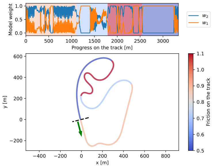
Driving on a track with varying speed: In this experiment, we drive the car following an optimized trajectory on a custom racetrack. We trained two models for frictions $\theta^{1}=0.5$ and $\theta^{2}=1.1$. The training data are collected by driving on the track with single surface friction and gradually increasing speed. At test time, there are three friction zones ($0.5,0.8,1.1$) and the proposed strategy computes the weight $w_{1}$ and $w_{2}$ using (6). The friction zones on the track and the weights used by EGP-MPC are shown in Figure 3. We can see that our controller is correctly choosing the GP models for the specific friction as the weights used in the ensemble correspond to the different friction surfaces. We compared the EGP-MPC with single GP-MPC and kinematic MPC controllers. Driving speeds and tracking errors are presented in Figure 5 and 4. The EGP-MPC is the only controller that successfully follows the trajectory while tracking the desired speed.

Testing on an unseen track: To show that the controller can generalize across multiple trajectories, we test the EGP-MPC that we trained in the previous experiment on the Sao Paolo ractrack shown in Figure 8. We do not retrain the models on any parts of the new track. The reference speed for this experiment is constant at $14$ m/s. As we can see in Figures 8 and 9, the algorithm is still able to perform well even when driving on a completely new track.

Lane change maneuver: We also test our algorithm on the standard dual lane change maneuver ISO3888-2:2011 2011. For this experiment, we train two new models by driving this maneuver at different friction coefficients: the first model is trained on data collected at a coefficient of friction $\theta^{1}=0.5$, while the second model is trained on data collected at a coefficient of friction $\theta^{2}=1.1$. For testing, we split up the maneuver into four segments of friction coefficients $[1.1,0.7,0.5,1.1]$. The reference speed is set to $15m/s$ and the proposed strategy computes the weight $w_{1}$ and $w_{2}$ using (6). Figure 6 shows the reference trajectory, friction coefficients of the trajectory, and the weight estimation by EGP-MPC. During the lane change maneuver, the dynamics of the vehicle are well excited. Therefore, the weight in the ensemble corresponds to the friction with less fluctuation than in Figure 9. A comparison of the tracking performance of different algorithms can be seen in Figure 7. It is important to underline that all tested algorithms except for the proposed EGP-MPC failed the lane change maneuver.

Effect of System Excitation In this experiment we demonstrate how the EGP-MPC works with 4 models and how system excitation can affect weight transition. Models are created from data collected at friction coefficients $\theta^{1}=0.5$, $\theta^{2}=0.6$, $\theta^{3}=0.9$, and $\theta^{4}=1.1$. We use the dual lane change maneuver described in the previous experiment. The target velocity is set to $15m/s$ and the maneuver is split into five segments of friction coefficients $[1.1,0.5,0.8,0.6,1.0]$. Friction segments and weight estimation by EGP-MPC algorithm are shown in Figure 10. Locations of the first two friction transitions are specifically chosen to demonstrate how weight estimation depends on the system excitation. The first friction change is during the turn. This corresponds to the spike in the lateral acceleration (orange line 1, middle graph, Figure 10), and immediate weight change (orange line 1, top graph, Figure 10). The second friction transition is on the straight line, so the system is not well excited (orange line 2, middle graph, Figure 10), and it takes much longer for the weight to start changing (orange line 2, top graph, Figure 10).

Computation time scaling Finally we discuss the runtime of the current implementation of the EGP-MPC algorithm. Because we are calculating the model ensemble before solving the MPC, the MPC solving time does not change with an increasing number of models (Figure 12). The current implementation calculates the linearization of models sequentially so the EGP-MPC computation time increases linearly (Figure 12). However, it is possible to compute this linearization in parallel which would improve computation time scaling with increasing number of models.

We observe three main limitations of our approach. First, the estimation of the weight vector as a convex combination limits the space of unseen parameters that can be modelled to the convex combination of the trained parameters. Secondly, the algorithm scales linearly in terms of computation time as the number of GPs increases. This can be improved by linearizing the GP in parallel through multi-threading or similar approaches. Finally, the weights estimated by the algorithm do not necessarily correlate with the actual value of the parameters of the system. This can be attributed to a lack of excitation of the system dynamics as can be seen when driving in straight lines at constant speed on the Sao Paolo racetrack (i.e Progress on the track 550m to 1000m).

References

- Agrawal et al. (2018) Agrawal, A., Verschueren, R., Diamond, S., and Boyd, S. (2018). A rewriting system for convex optimization problems. Journal of Control and Decision, 5(1), 42–60.
- Althoff et al. (2017) Althoff, M., Koschi, M., and Manzinger, S. (2017). CommonRoad: Composable benchmarks for motion planning on roads. In 2017 IEEE Intelligent Vehicles Symposium (IV), 719–726. IEEE, Los Angeles, CA, USA. 10.1109/IVS.2017.7995802.
- Betz et al. (2022) Betz, J., Zheng, H., Liniger, A., Rosolia, U., Karle, P., Behl, M., Krovi, V., and Mangharam, R. (2022). Autonomous vehicles on the edge: A survey on autonomous vehicle racing. IEEE Open J. Intell. Transp. Syst., 3, 458–488. 10.1109/ojits.2022.3181510.
- Christ et al. (2021) Christ, F., Wischnewski, A., Heilmeier, A., and Lohmann, B. (2021). Time-optimal trajectory planning for a race car considering variable tyre-road friction coefficients. Vehicle system dynamics, 59(4), 588–612.
- Diamond and Boyd (2016) Diamond, S. and Boyd, S. (2016). CVXPY: A Python-embedded modeling language for convex optimization. Journal of Machine Learning Research, 17(83), 1–5.
- Gardner et al. (2018) Gardner, J., Pleiss, G., Weinberger, K.Q., Bindel, D., and Wilson, A.G. (2018). Gpytorch: Blackbox matrix-matrix gaussian process inference with gpu acceleration. In S. Bengio, H. Wallach, H. Larochelle, K. Grauman, N. Cesa-Bianchi, and R. Garnett (eds.), Advances in Neural Information Processing Systems, volume 31. Curran Associates, Inc.
- Hewing et al. (2018) Hewing, L., Liniger, A., and Zeilinger, M.N. (2018). Cautious nmpc with gaussian process dynamics for autonomous miniature race cars. In 2018 European Control Conference (ECC), 1341–1348. IEEE.
- Hewing et al. (2020) Hewing, L., Wabersich, K.P., Menner, M., and Zeilinger, M.N. (2020). Learning-based model predictive control: Toward safe learning in control. Annual Review of Control, Robotics, and Autonomous Systems, 3, 269–296.
- ISO3888-2:2011 (2011) ISO3888-2:2011 (2011). Passenger cars–test track for a severe lane-change manoeuvre–part 2: obstacle avoidance.
- Jain et al. (2021) Jain, A., O’Kelly, M., Chaudhari, P., and Morari, M. (2021). Bayesrace: Learning to race autonomously using prior experience. In J. Kober, F. Ramos, and C. Tomlin (eds.), Proceedings of the 2020 Conference on Robot Learning, volume 155 of Proceedings of Machine Learning Research, 1918–1929. PMLR.
- Laurense et al. (2017) Laurense, V.A., Goh, J.Y., and Gerdes, J.C. (2017). Path-tracking for autonomous vehicles at the limit of friction. In 2017 American control conference (ACC), 5586–5591. IEEE.
- Le and Nghiem (2021) Le, V.A. and Nghiem, T.X. (2021). A receding horizon approach for simultaneous active learning and control using gaussian processes. In 2021 IEEE Conference on Control Technology and Applications (CCTA), 453–458. 10.1109/CCTA48906.2021.9659046.
- O’Kelly et al. (2020) O’Kelly, M., Zheng, H., Karthik, D., and Mangharam, R. (2020). F1TENTH: An Open-source Evaluation Environment for Continuous Control and Reinforcement Learning. Proceedings of Machine Learning Research, 13.
- Pleiss et al. (2018) Pleiss, G., Gardner, J., Weinberger, K., and Wilson, A.G. (2018). Constant-time predictive distributions for Gaussian processes. In J. Dy and A. Krause (eds.), Proceedings of the 35th International Conference on Machine Learning, volume 80 of Proceedings of Machine Learning Research, 4114–4123. PMLR.
- Ragan-Kelley et al. (2017) Ragan-Kelley, J., Adams, A., Sharlet, D., Barnes, C., Paris, S., Levoy, M., Amarasinghe, S., and Durand, F. (2017). Halide: decoupling algorithms from schedules for high-performance image processing. Communications of the ACM, 61(1), 106–115. 10.1145/3150211.
- Rodriguez et al. (2021) Rodriguez, I.D.J., Rosolia, U., Ames, A.D., and Yue, Y. (2021). Learning to control an unstable system with one minute of data: Leveraging gaussian process differentiation in predictive control. In 2021 IEEE/RSJ International Conference on Intelligent Robots and Systems (IROS), 3896–3903. IEEE Press. 10.1109/IROS51168.2021.9636786.
- Rosolia and Borrelli (2020) Rosolia, U. and Borrelli, F. (2020). Learning how to autonomously race a car: A predictive control approach. IEEE Transactions on Control Systems Technology, 28(6), 2713–2719. 10.1109/TCST.2019.2948135.
- Rosolia et al. (2018) Rosolia, U., Zhang, X., and Borrelli, F. (2018). Data-driven predictive control for autonomous systems. Annual Review of Control, Robotics, and Autonomous Systems, 1, 259–286.
- Stellato et al. (2020) Stellato, B., Banjac, G., Goulart, P., Bemporad, A., and Boyd, S. (2020). OSQP: an operator splitting solver for quadratic programs. Mathematical Programming Computation, 12(4), 637–672. 10.1007/s12532-020-00179-2.
- Van Gennip (2018) Van Gennip, M. (2018). Vehicle dynamic modelling and parameter identification for an autonomous vehicle. Master’s thesis, University of Waterloo.
- Vaskov et al. (2022) Vaskov, S., Quirynen, R., Menner, M., and Berntorp, K. (2022). Friction-Adaptive Stochastic Predictive Control for Trajectory Tracking of Autonomous Vehicles. In 2022 American Control Conference (ACC), 1970–1975. IEEE, Atlanta, GA, USA. 10.23919/ACC53348.2022.9867523.